Collaborative solar powered neighborhoods

Collaborative Solar Powered Neighborhoods

AR

Georgetown University, 2010

LIB

SUBMITTED TO THE DEPARTMENT OF MATERIALS SCIENCE AND ENGINEERING IN PARTIAL FULFILLMENT OF THE REQUIREMENTS FOR THE DEGREE OF

MASTER OF SCIENCE IN MATERIALS SCIENCE AND ENGINEERING

AT THE

MASSACHUSETTS INSTITUTE OF TECHNOLOGY

JUNE 2015

C Massachusetts Institute of Technology 2015. All rights reserved

SErTT INSTITI ITF CHNOLOLGY

17

2015

RARIES

_Si

S

Signature redacted

Siar

Department of Materials Science and Engineering

ature redacted

Jeffrey Grossman Professor of Materials Science and Engineering

-- Thesis Supe~rvisor Thesis - Suevio Nicola Ferralis Research Scientist Thesis Supervisor Donald R. Sadoway on Graduate Students

gnature redacted

ignature redacted

Collaborative Solar Powered Neighborhoods

by

Anna Cheimets

Submitted to the Department of Materials Science and Engineering on May 22, 2015 in Partial Fulfillment of the Requirements for the Degree of Master of Science in

Materials Science and Engineering

ABSTRACT

Solar photovoltaic (PV) deployment has been steadily expanding over the past decade. While decreasing our reliance on fossil fuels will be beneficial for the environment, increasing our exposure to an intermittent renewable resource could have negative consequences on the electric grid. There can be oversupply

conditions at midday when PV is outputting at peak power and also steep ramping of fossil fuel plants when PV is coming on or going off line. In this project, we investigated how to use more of the three-dimensional landscape of a residential neighborhood to flatten and lengthen the PV power profile. We built small modular houses with solar panels to characterize different configurations of solar panels and reflectors. We designed and built a set of I-V curve measurement instruments to allow us to collect separate I-V curve measurements from the difference faces of the experimental houses. We found that placing solar panels on the east and west facing roofs and walls of houses expands the power profile but it also leads to more inter-house shading which we quantified in our experiments. We attempted to mitigate the shading by placing reflectors on adjacent house roofs and walls but determined that the added energy from the reflectors was far less than would have been

produced by solar panels in the same location. Finally, we placed reflectors on the ground and quantified the improvement in power and energy generation of the walls they abutted. Taken together, our findings give us the beginnings of a suite of techniques to apply to real neighborhoods with the aim of broadening the PV power profile and enabling solar panel deployment in previously overlooked areas.

Thesis Supervisor: Jeffrey Grossman

Title: Professor of Materials Science and Engineering Thesis Supervisor: Nicola Ferralis

Acknowledgements

I would first like to thank my advisors Professor Jeff Grossman and Dr. Nicola

Ferralis for coming up with the overarching vision for the project. Thank you to Jeff for always helping me see and frame the big picture whenever I started getting lost in the weeds. Thank you to Nicola for helping to guide me through the experimental process. I have learned so much for being a part of the Grossman group.

There are a number of people who helped me tremendously with my experimental setup and analysis. A big thank you to David Bono for all of the time he spent working with me on understanding and then designing and building the excellent measurement instruments for collecting power data from my setup. Thank you to

Kevin Connelly for allowing me to have access to the roof for experiments and for unlocking the door for me so many times. Thank you to Tomi Adelusi, my

undergraduate research assistant, who did all of the computer simulations of my experiments and was a constant source of ideas. Also, I thank David Berney

Needleman and Rupak Chakraborty for allowing me to build on their hardware and software for collecting power for solar cells.

I would like thank all of my amazingly intelligent and caring classmates in DMSE. I

would not have made it through all of our core classes without studying and commiserating with them.

Thank you also to the Grossman group for being such a supportive and welcoming lab group. I couldn't have asked for a better environment in which to work.

I would like to thank my family for always being so supportive of me. They are each

my role models in different ways.

Lastly I would like to thank Alex for always being there when I need him and for filling my life with love, adventure and conversation.

Table of Contents

Acknow ledgem ents ... ₅

Introduction ... ₉

Solar Cell Operation ... ₁₃

3D PV Concept and Previous Research ... 15

Experim ental H ardw are ... 18

M easurem ent channels ... ₁₈

Neighborhood hardw are ... 27

Results and Discussion ... ₃₁

Testing assum ptions ... ₃₁

Error analysis ... 33

Results ... ₃₆

Varying house orientation ... ₃₇

House-m ounted m irrors ... 45

House-m ounted diffuse reflectors ... 48

Ground m ounted m irrors ... 52

Ground-m ounted diffuse reflectors ... ₅₄

Conclusions ... ₅₇

Future w ork ... 60

References ... ₆₁

Introduction

Over the last decade and a half, the U.S. has experienced a huge increase in installed capacity of solar photovoltaics (PV). Figure 1 shows the annual PV capacity

installed in the U.S. since 2000 for residential, non-residential and utility scale applications [1]. 6.201 6.000 5.000 4.776 4,000 3,369 3.000 1.922 2,000 1,000 852 4 11 23 45 58 79 105 160 298 382 2000 2001 2002 2003 2004 2005 2006 2007 2008 2009 2010 2011 2012 2013 2014

m Residential m Non-Residential 0 Utility

2015 AU~c

Figure 1: Annual PV capacity installed in the U.S. since 2000. PV capacity has been increasing rapidly in the last fifteen years. [1]

While PV and other renewable energy sources such as wind have many

environmental benefits, they are by their nature intermittent electricity sources and somewhat unpredictable [2]. This variability makes it difficult for grid operators to precisely balance the load and supply in the system [3]. In addition, since PV

normally peaks in the middle of the day when the sun is at its highest point, the non-renewable electricity sources must be ramped down and then up quickly as the sun is rising and setting. This type of repeated cycling of fossil fuel plants shortens their lifespans and increases their operation and maintenance costs [2].

In some places, like Hawaii with high PV penetration, there has already been push back from electric utilities about installing more rooftop solar. The influx of power from private homes can create instability on the grid and damage equipment if not handled properly [4].

Potential solutions to the managing the extra power and intermittency include major upgrades to the grid infrastructure, high capacity batteries or super

capacitors, or curtailing solar power at certain times of the day, among others [5]. These can be very expensive, technologically challenging or unpalatable options. Although grid-level storage is highly appealing, to date no technology apart from pumped hydro has been shown to scale effectively. However, apart from the possibility of storage, given the importance of the problem it is crucial to consider other routes to developing inexpensive approaches that stabilize and minimize power fluctuations generated by PV. In this thesis, we consider the following question: Instead of treating each residential installation separately, can we have panels or mirrors or reflectors on different neighboring houses interact to provide more even power from PV over the course of a day?

There are two main reasons why this is a relevant question to ask now. The first reason is that the prices of solar panels have dropped by more than 70% in the last decade and a half [6]. Figure 2 shows the installed system price of residential and commercial PV along with the global module price index from 1998 to 2013.

$14 leeldtlalA COew M

(Median Vos)

$12 - - -10okW

- -= -M10-100 kw

.2 $0

ftM nw1V n*0 nal" n.441 n*q4IO8 no6U7 rwlff wuO "u17,64 nuIAM n=34,319 nu646 n*4238O a41.75 n*M,64

Inetalladn Yaw

Figure 2: U.S. installed PV system prices and global module price index since 1998. By 2013, th module price was almost 20% of the cost of an installation [6].

By the end of 2014, the module price was only 21% of the installed price of the

residential solar installation in the U.S.[1]. This gives us the flexibility to place solar panels in configurations that do not necessarily optimize for energy generation on a per panel basis. We can thus afford to add extra solar panels to increase the length of time the solar installation is generating power throughout the day.

The second reason this is a pertinent question is that we can build upon earlier research that investigated optimized three-dimensional shapes for stand-alone solar panel installations [7, 8]. The structures considered were made from closely spaced panels pointing in different directions, and it was found that such 3D structures provided a flatter and wider energy profile over the course of the day than a horizontal panel with the same areal footprint as the 3-D structure. While these earlier studies helped to lay the groundwork for the potential benefits of 3DPV, such structures pose challenges at larger scales related to stability and cost. On the other hand, the landscape of already existing 3D structures - namely buildings - provides an interesting opportunity to expand upon the 3DPV concept, and to explore the potential of using this fixed landscape to enhance power collection and uniformity. The goal of this thesis is to explore the use of the existing 3-D landscape of a

neighborhood to replicate previous the findings from single 3D structures on an urban scale.

In the course of this work, we designed and built measurement channels to measure the power generated by small neighborhoods of model houses placed outside. We varied the neighborhood configurations by adjusting the spacing and orientation of the houses and by adding mirrors and diffuse reflectors. We then characterized the power generated by the inter-house interactions in the neighborhoods.

We came to the following conclusions over the course of this study:

- Placing panels on east and west facing roofs, and unobstructed east and west facing walls, increases the amount of time for high PV power output.

- Placing a house covered in either diffusely reflective tape or mirrors next to a house covered in solar panels increased the energy generation of the panels. However, that added energy could be much more efficiently generated by a much smaller area of solar panels.

- Placing the same diffuse reflectors or mirrors on the ground between houses covered in solar panels increases the energy generated by the solar panels on the walls without displacing solar panels.

The mirrors and diffuse reflectors used in this study increased the energy

generated by the solar panels by about the same amount. The mirrors increased the power mostly in the middle of the day, while the diffuse reflectors increased the power throughout the day.

In the future, software and experimental improvements on our platform will

extend our understanding on how different types of neighborhoods might benefit from this method of using building interaction to improve PV performance.

As a result of our experiments, we have characterized the power and energy

changes that come from different types of inter-house interactions in a neighborhood. We used these interactions to provide more uniform power to the grid from PV.

Solar Cell Operation

A photovoltaic (PV) cell converts electromagnetic radiation into electricity. While

several PV commercial architectures exist crystalline silicon (c-Si) cells make up the largest share of them with 90% of the market [9]. Since the focus of this work is on how solar cells are distributed in a 3D space, rather than the performance of a particular PV architecture, for simplicity the solar cells used in this research are c-Si cells. Given the generality of the approach, any of the results here presented can be

immediately be translated for a given PV technology.

The basic structure of a solar cell is shown in Figure 3 below from pveducation.org.

antirefecton coating

611 Mifrtonftct

mher

food; bar

rear contact

Figure 3: Schematic detailing how a solar cell works. Electromagnetic energy from the sun hits the cell and generates and electron hole pair. The cell separates the two opposite charges in order to power an external load [9].

The top layer is glass with an anti-reflective coating to improve light absorption. The second layer is emitter layer. Light entering this region excites charge carriers, an electron (a negatively charged carrier) and a hole (a positively charged carrier). The holes are swept across to the collector layer and the electrons travel through the external circuit to power a load. For a more detailed description of the function

of a solar cell, see pveducation.org.

In order to assess the performance of individual or an assembly of solar cells throughout the day, we measure the power that the solar panels are generating at any given time. The amount of power the solar panel can deliver to an external circuit depends on the size of the load that the solar panel is powering. For any

solar panel there is a load size that maximizes the amount of power the solar panel generates. This is called the maximum power point (MPP). We calculate the power generated by a solar panel by multiplying the current it is generating by the voltage applied across it. In order to find the maximum power value we need to measure the current the panel generates across a range of applied voltage values. This is called the current-voltage curve or I-V curve [9].

Figure 4 is plot of a typical I-V curve from pveducation.org.

IV of the solar cell

C

Power from the solar cell

Voltage _VOC

Figure 4: This is the relationship between the current and voltage generated by a solar cell, called the current-voltage or I-V curve. The power is the product of the voltage and the current.

When the product of current and voltage applied is plotted over the voltage applied, the maximum of the curve will be the MPP. For the remainder of this thesis, we will refer to MPP as power generated.

3DPV Concept and Previous Research

A previous study by Meyers et al investigated the question: What is the

optimal shape of a three dimensional photovoltaic device confined to a given volume? How much more energy could be generated with this 3D configuration than with a flat panel the size of the horizontal footprint? In Meyers et al (2010), the researchers wrote a computer algorithm to optimize a 3D photovoltaic (3DPV) structure for maximal energy generation and minimal inter-cell shading in a confined space [7]. Their code generated a structure that resembled a cube with funnels on all faces. Figure 5a is the shape generated by their algorithm and Figure

5b is a simplified funnel shape that retains much of the improved performance.

(a)

(b)

Figure 5: a) Optimized shape for collecting solar power in a given volume. b) Simplified version of the optimized shape [7].

Bernardi et al improved the 3DPV concept through additional computational and experimental tests. In both papers computational algorithms were employed to simulate and optimize the 3DPV structures, although in the work of Bernardi et al the algorithms were further improved and the first structures were built in order to experimentally validate as well as understand a further explore the 3DPV concept

(a)

Figure 6: PV structures built to validate the simulation results for 3DPV [8].

They measured the amount of energy generated by each structure per unit base area and compared that to the energy generated by a flat horizontal panel with the same base area. When tested under real insolation conditions, the experimental 3DPV structures, generated 2-20 times more energy per unit footprint area than a flat panel tested at the same time with clear skies. According to their calculations, the 3DPV structures outperformed the flat panel the most at higher latitudes and in the winter when the light rays are at the lowest angle. In addition, the experiments

revealed that taller structures produced considerably more energy per unit base area on cloudy days than the flat panel. The tower performed the best in this situation (i.e., overcast skies) as it produced about 40 times more energy than the flat panel even though it was made up of only 32 panels. In addition, it was found that the 3D structures produced at their peak power levels for more than twice as long as the flat panel did. Finally, the computational algorithm predicted optimal shapes for 3DPV structures that used mirrors to dynamically enhance the power to several solar panels.

These findings have a number of important implications for real-world PV implementation. First, while the energy produced per unit active solar panel area is

lower for the 3D structures, solar panel prices are decreasing and are now only 21% percent of the total cost of a PV installation [1,6]. Where ground area is valuable, a 3DPV structure may be more cost effective. Second, power from PV is low or

intermittent on cloudy days. A technology that could make PV more resilient to bad weather would greatly improve reliability. Finally, power from PVs is constantly

changing as it increases while the sun rises and decreases as it sets. The impact from the significant variability of solar power availability in relation to demand, requires power utilities to constantly ramp up and down other grid-level power sources to compensate. Such power sources are notoriously not resilient to transients in operation with increases in operative costs [2]. 3DPV structures produce power for longer periods at their peak power, similar to dual axis tracking systems [8] but without moving parts, which would further improve their reliability as a long-term power source. Furthermore, 3DPV structures could be foldable and easily deployed to serve as reliable sources of power either on or off grid.

The focus of the research discussed in this thesis is based on applying the 3DPV concept to the existing three-dimensional architecture of buildings and residential neighborhoods. The configurations studied in the previous research were not constrained to any particular shape and thus pose additional cost and durability challenges. For the work described in this thesis, we wanted to take advantage of the existing 3D landscape of neighborhoods in order to recreate the same type of power profile broadening. To do this, we looked at three main variables:

- House orientation (N,E,S,W) - Inter-house shading

- House mounted reflectors (both diffuse and specular)

Experimental Hardware

Measurement channels

In order to compare the output of different panel configurations, we needed to measure the power generated different groups of solar cells at the same time. We designed an instrument, which we will call a measurement channel or channel, that could take the current-voltage (I-V) curve of groups of cells at regular intervals,

calculate the maximum power generated, and record all of the data onto SD cards for later analysis. Eight of these channels collected data during the experiments.

Sophisticated equipment for measuring power generated from solar arrays was available but was either too expensive to purchase in large numbers or was not

suited to our specific application. Each group of solar panels connected to each measurement channel in our experiments could produce on the order of 1 Amp of current at about 8 volts which is considerably more power than lab scale cells but less power than commercially available panels for residential installation. This is reason we needed a customizable instrument that could log weeks of data without user input.

The final measurement channel was designed to be robust, safe and accurate, and straight-forwardly retooled to use with different sized cells. The design for our channel was based on a simpler device that worked with much smaller cells. This simple device used an Arduino as the controller to allow facile programming and had circuitry that we would adapt to use with larger solar cells. David Berney Needleman and Rupak Chakraborty in Professor Tonio Buonassisi's group at MIT designed the original circuit and some acquisition software. We took their basic concept and added an on-board power supply, an amplifier and a number of

circuitry changes to make an Arduino controlled instrument that could characterize panels generating up to 3 A at up to 8 v. Additionally, we integrated their

acquisition code into the SolarLogMeter, software written by Nicola Ferralis in order to automate data acquisition and storage [11].

In brief, the instrument works by ramping up a voltage across the solar panels and then measuring the voltage drop across a small resistor caused by the

current generated by the panels. This is a commonly used method for measuring the I-V curve of solar cells [10]. Because the Arduino and the other original circuit components could only deliver a maximum of 5 v and less than 50mA, we built in a bipolar power supply to deliver up to 11 v and an amplifier to sink up to 3 A from the illuminated panels.

Measurement Channel Hardware

Overview

Figure 7 shows a schematic of the instrument's function.

Analog signal

Digital signal

000

Figure 7: Schematic showing the function of the measurement channels. The computer was only used to load the program onto the Arduino at the beginning of use. There was no computer needed for the channels to function.

The Arduino controls a voltage applied across the group of solar panels connected in parallel. We will call this collection of panels the device under test

(DUT). As this reverse bias voltage is increased, the magnitude of the current output

of the DUT decreases to zero as the applied voltage approaches the open circuit voltage. The current generated by the DUT drops across a small resistor and creates a voltage. This voltage is then amplified and directed back to an analog input in the Arduino. The software programmed into the Arduino uses this voltage data to calculate the amount of current generated by the cell. The Arduino also

simultaneously measures the voltage drop across the DUT. This current and voltage data can then be plotted as the I-V curve. The instrument automatically takes an I-V curve every 12 minutes but this time interval can be easily changed. Each IV curve

is stored in one file and the maximum power generated is calculated from each curve and then stored in a separate file for ease of data analysis.

Arduino and Digital to Analog Converter (DAC)

In Figure 8 we show detailed schematic highlighting the part of the circuit that controls the voltage sweep. See the appendix for the full circuit diagrams for the measurement channel.

4

Serial data

fom Adulejt y

wo Th

-Figure 8: Left: Circuit diagram showing the part of the measurement channel circuitry that controls the voltage sweep. Right: The relevant circuit components highlighted In yellow.

We used an Arduino Mega 2560 microcontroller for this project. It provided

10 bits of resolution-1024 different voltage values between 0 and 5 V at its analog

inputs-which was enough for the purposes of these experiments.

The Arduino communicated with the DAC to output two separate voltages. The first voltage was the ramp voltage applied across the DUT. The second voltage was a constant voltage supplied to the summing amplifier that will be discussed later.

We used an MCP4822 DAC which had two 12 bit voltage outputs that could each supply up to 4.1 V.

Power Amplifier

The DUT operated at a much higher current and voltage than the DAC could put out itself so we built an amplifier to supply the required current and voltage. This differential voltage power amplifier had a gain of 2 and could provide up to 8 V and 2 A to the circuit. Figure 9 is a schematic of the differential amplifier which is the voltage amplification part.

To DUT

Power

ampifier

Figure 9: Circuit diagram and photo of the power amplifier of the measurement channels

The relative values of the four resistors determines the gain (see Appendix for the full circuit diagram). In this case, because the values of R9 and R7 are equal as are the values of R13 and R3, the governing equation for the gain is simplified to the following equation:

Gain=R13/R9=R3/R7

The current amplification part is required because the groups of solar cells in the experiments generate up to 1 Amp, which is far too high for the op-amp in the

differential amplifier to sink or source on its own. In addition, we needed a circuit element to block the current generated by the DUT from damaging the DAC. We built a bipolar triple Darlington emitter follower power amplifier to sink and source current with low distortion and high bandwidth operation. To understand what this means, we can break this down into its important features.

First, the bipolar nature of the amplifier means that this instrument can be used for current traveling in both directions. Taking a full I-V curve requires operation in both regimes. If a cell is illuminated and the instrument applies a forward bias less than the open circuit voltage of the cell, the current will flow from the positive electrode through the amplifier and out to the power supply. If the instrument applies a forward bias higher than the open circuit voltage, the current will go the other way-from the negative terminal, through the amplifier and out through the power supply. Transistors Q1-Q3 are NPN type and draw power from the positive power supply, while transistors Q4-Q6 are PNP type and draw from the

negative power supply (see full circuit diagram in Appendix).

Second, the amplifier is designed to supply current immediately when voltage is applied to the cell and to minimize distortion of voltage and current.

When using transistors in a power amplifier, a certain voltage must be applied at the base of the transistor for it to turn on and begin amplifying the current. These transistors require 1.3 V at the base to turn on. To address this, diodes D3-D8 were placed in series to provide a constant bias voltage. This voltage supplies a constant bias current through the driving transistors Q2 and Q5 (see fill circuit diagram in Appendix). This reduces crossover distortion, which is inaccurate current output when the current changes directions and must flow through the opposite set of transistors.

Summing amplifier

We can use an Arduino to measure current on the order of amps generated

by the solar cells if we measure the resulting voltage from dropping the current over

a small resistor. We need to use a very small resistor (R23 in the circuit diagram in the Appendix) called a shunt to avoid putting a significant load on the cells and as a result we will have a small voltage drop.

There are two challenges to measuring the voltage drop across the shunt, R23. The first is that the voltage may be small under poor cell illumination, on the order of a few millivolts in low light conditions, which may fall below the noise at the analog inputs of the Arduino. The second challenge is that when the cells are

negative. Feeding a negative current directly into the Arduino or an op-amp will damage the circuit elements.

We solve these two challenges with a summing amplifier show in Figure 10.

Current from DUT

Summing W amplifier 4 R21_12k F Load istor To ground To Arduino

Figure 10: circuit diagram and highlighted photo of the summing amplifier in the measurement channels.

This circuit element adds a positive constant voltage to the negative voltage generated by the solar panel current and it also amplifies the resulting voltage for the Arduino to read. The DAC supplies the constant positive voltage from the output port Vb. The equation governing the output voltage from the summing amplifier as function of the input voltages is as follows:

Vout=[Vin* R21/(R21+R20) + Vb*R20/(R21+R20)] * [1+R22/R24]

The resistor and Vb values were chosen to accommodate a current range from 0-2.5A. Because of the large current range, the resolution is about 2.9 mA.

Voltage measurement

The Arduino measures the voltage applied to the DUT at the DUT's positive terminal. A voltage divider formed by resistors R1 and R6 splits the voltage in half to accommodate the Arduino's analog input range of only 0-5 V. Figure 11 is the cicuit diagram of the voltage divider.

From DUT IP2 AO Voltage divider R2 4&~ 2 1 .J R~5 4939 D2 1N?52 To Arduino analog input

Figure 11: Circuit diagram of the voltage divider in the measurement channels.

Power supply

The on-board, bi-polar power supply delivers three separate voltages and up to 3A of current to the circuit. The current is limited to 3A by the transformer and the voltage regulators. The benefit of having the onboard power supply is that each measurement circuit can be plugged directly into the wall without the need for more bulky equipment. In addition, the 3A limit on this power supply is a built-in safety feature that prevents a huge current draw in the case of a short or malfunction. The

5v output powers the DAC and the Arduino, while the 11.3v and -11.3v outputs power the op-amp and the power amplifier.

Data Storage

We purchased a preassembled data logging shield from Adafruit that plugs into the Arduino to save the collected data on an SD card [12]. The board has a real time clock (RTC) that puts a time stamp on each reading and a small battery to keep the RTC running when power is turned off.

Measurement Channel Software

One significant advantage of using an Arduino to control the measurement channels is the freedom and ease of programming it. The code was specifically designed to acquire and store data from the DUT and from a silicon photodiode for irradiance measurements. The SolarLogMeter includes calculations to translate the voltage signals at the analog inputs into the actual current and voltage values from

the DUT. It determines the maximum power point, fill factor, short circuit current and open circuit voltage from each IV curve. It also calculates the position of the sun based on the time of day and records it along with the acquisition data.

Currently the code has more functionality than the hardware, leaving open the option for future hardware improvement. For example, while temperature and barometric pressure can be recorded with SolarLogMeter, they are not recorded in the experiments in this thesis. In addition, the code was built to automatically adjust the gain of the summing amplifier giving the channel the best resolution possible for every light level. The hardware does not currently support this function which will supported in future versions.

Voltage calculation

The Arduino receives the analog voltage at its analog input and translates it into a digital signal through its ADC. Our code back calculates the applied bias voltage from this digital signal. The Arduino performs the calculation as follows:

Vapp=D *(5volts/1024bits) * 2

Where Vapp is the voltage applied to the DUT and D is the digital signal from the Arduino's ADC. We multiply by 5/1024 because the Arduino has 10 bit

resolution over its 5 volt input range. That is, it breaks up the 5 volts into 1024 segments. We multiply by 2 because used a divide-by-two voltage divider to reduce the voltage entering the analog input.

Current calculation

The current generated by the panels flows from ground, across R23 and back through the power amplifier. As discussed previously, we are measuring the voltage across R23 so that we can calculate the current that dropped across it. However, the voltage that measured by the Arduino at the analog input is the voltage output from the summing amplifier. Therefore, we first need to convert the digital signal from the ADC into a voltage value, then use the equation for the summing amplifier to

calculate the voltage across R23 and lastly we need to divide this voltage by the resistance of R23 to arrive at a current value.

The equation for calculating the current is as follows: I=D*(5volts/1024bits)*1/[(1+R22/R24)*R21/(R20+R2 1)]-Vb[R20/(R20+R21)][1+R22/R24] * 1/R23

The maximum power point is calculated by multiplying the measured voltage and current values together and then picking the maximum value.

Calibration

Each measurement channel must be calibrated before its first use because of the limited precision of the circuit elements. To determine the offset, we run an open circuit IV sweep (i.e. without panels connected to the measurement system) and assume that the resulting reading is a measurement of zero current. We save each unique offset on each channel's SD card and subtract it from all of the readings.

The main source of the offset is the imprecision of the constant voltage Vb delivered by the DAC. The Arduino current calculation is very sensitive to the value of Vb so the small offset and gain offset error of the DAC shifts the calculated current value. The ADC in the Arduino also has a small offset error that seemed to have less impact than the DAC's. Over the course of the experiments, the calibrations

remained fairly stable. A couple of channels were recalibrated over the course of the experiments.

Measurement Channel Future Work

The instruments would benefit greatly from the ability to wirelessly transmit the data from their remote location, rather than saving it locally into a SD card. They might either constantly stream the data to a server or they could allow a

remote user to login and download the stored files. This would save time for the user if the DUT is in a hard-to-access location and it would alert the user to any problems with data acquisition.

As the instrument is currently designed, it can only serve as a single

measurement channel; it tracks the data from a single set of panels. However, the Arduino Mega has enough ports to track data from four sets of panels. If we make

the circuit design more compact, we could fit more channels into one box. The circuit design for the current instrument is intentionally not very dense to facilitate assembly and testing.

As mentioned earlier, the Arduino code has the functionality to automatically detect the current and adjust the gain accordingly to achieve the best resolution. A future version of hardware could have this capability. We could install three resistors with different values to serve at R22. Changing the value of this resistor will adjust the gain of the summing amplifier. These resistors would be connected

to the circuit by switchable transistors controlled by the Arduino. The Arduino would also adjust the value of Vb, the constant voltage added to the signal in the summing amplifier. We add a lower voltage if we have a lower current. For

example, if we knew we were only generating a current of 500mA, we could switch R22 to 20,000 ohm (from 6040 ohms) and switch Vb to 0.25volts (from 1volt) and we would have a resolution of about 1 mA instead of about 3 mA.

The instrument would also benefit from a self calibration function. We could build in a switch that would disconnect the solar cells and take a baseline zero

current measurement. The code would then use this as the offset and incorporate it into the current calculation. Alternatively, we could measure the exact value of Vb at all times using an analog input on the Arduino and use that in each current calculation instead of the programmed value. This would eliminate the largest source of the offset in the current measurement.

We built a robust and customizable instrument for measuring and logging the IV curves from small arrays of solar cells. Each channel can handle up to 3 amps from the DUT and can be plugged straight into a standard wall outlet for power. This power range is applicable for hobby and lab sized solar arrays and could be custom designed easily to accommodate different expected current ranges within the upper limit. The Arduino software can be readily adopted to different test protocols. If we incorporate the suggested improvements, this instrument could be a very useful tool for educators, hobbyists, researchers and engineers.

Neighborhood hardware

House design

The overarching principles of the design of the house and panel mounts were flexibility and modularity. The construction process needed to be able to easily accommodate different configurations, considering that future testing might require an assembly that was not originally planned. The full model house design consisted of the following components:

- House

- Solar panel mounts - Wire management

The houses are built from two types of PVC extrusions. The house bodies were made from 2" by 4" rectangular tubes, and the roofs were made from 900 angle extrusions with 3 " side lengths. The PVC tubes were easily cut into regularly sized house building blocks and held together with flexible Zipties.

The solar panel mounts can rotate and then lock in place, enabling great flexibility in solar panel orientation choice. The experiments described in this report do not make use of this extra degree of freedom yet, though future work will. The manufacturer of the mounts intended for them to be dashboard mounts for cellphones but they were just the right size to accommodate the panels in the experiment.

The final aspect of the house model was the wire management. Each house contained 24 solar panels which had to be connected to each other and protected from rain, ice and snow. Keeping in the spirit of flexibility and modularity, the panel connections needed to be sturdy but also easily rearranged for different panel and house configurations.

All six panels on each house face were connected together in parallel. The wires

from the panels traveled down the center line of each of the houses' faces and were bundled together with nylon twist ties. Once bundled, the wires plugged into bus bars using quickly disconnecting MTA connectors. Six panels connect to one bus. In certain experiments, two busses were connected together to put two house faces on one measurement channel.

To keep the wires safe from water, each bus bar tucked into a narrow plastic sheath with duct tape covering the top opening. The sheaths were originally travel

toothbrush holders and were very well sized for the application. All four bus bar packages slid under the roof of the house and remained accessible without taking apart the house. The wires remained dry throughout the entire winter of deep snow, high wind and heavy rain.

Solar cells used in these experiments are Solarbotics SCC3766 [13]. The monocrystalline silicon panels are 37mm by 66mm in size with an average

efficiency of -14.0%. In full sun, the Voc is 8 volts and the Isc was about 45 mA [14]. We measured the efficiency of each of the solar panels using a solar simulator to ensure there were no duds and to better understand the expected error in the experimental results.

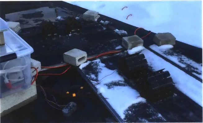
Cases for measurement channels

The measurement channels were placed in large plastic bins for protection from the elements (see Figure 12). Four channels fit in each bin. We punched holes in the bottom to run wires in and placed the bins up on cinder blocks to avoid any

possibility of flooding. We ran an extension cord from the outdoor electrical outlet into each bin and connected to power strip with an on/off switch.

The four measurement channels in each box plugged into the power strip. The data logging could easily be reset between experiments using the power switch. A cinder block on the top of each bin

provided more ballast to keep the bins from

Figure 12: The box with the measurement blowing over. The bins sat on the north

channels.

side of the houses in the experiments to avoid shading them.

Test platform

The house models were placed securely on platform during the experiments to keep them steady and dry. We used a polypropylene peg board framed by aluminum t-slotted framing and ballasted with cinder blocks. The regularly spaced holes in the peg board made experiment set up and alignment easier. We screwed tie down loops directly into the peg board and tied the houses down with cord.

Figure 13: Left, A house on the platform. Right, the tie down mechanism.

This system worked reasonably well but screwing in the tie down loops was

occasionally tedious time consuming. The setup would have been greatly improved with a quick connect system of some kind, especially considering the setup was sometimes done in the dark in freezing temperatures.

Location

The test setup was located on the roof of Building 3 at MIT. The experiment

received unblocked sun for all but about one hour in the morning when the sun was behind a building. There was no shading from the rooftop HVAC system. The roof entrance was easily accessible and the space was enclosed by short walls that made it safe to be up there without supervision.

Results and Discussion

We performed experiments to test the feasibility of using solar panel and mirror placement to tune the power generation profile of adjacent houses in a

neighborhood. As mentioned previously, the goal of the project was to increase the extent of the time in a day that a neighborhood can generate a steady supply of electricity. Our aim was to learn about the interactions that the houses had with each other with regard to reflections and shading so that we could understand how to tune the power profile of a neighborhood in a relatively inexpensive way. Each test involved one or two neighborhoods of two to three simplified, scaled down models of houses with solar panels, mirrors or reflectors. Whenever possible, we tested ways that we could use reflective materials that would be considerably cheaper and easier to install than solar panels.

All the testing was done outdoors on the roof of Building 3 at MIT, from November

to May. As a result, the lighting in all the experiments is variable over the day and over the months, as it would be under realistic weather and seasonal conditions. To remove this variability as much as possible from the results, each test neighborhood was usually only compared to a suitable control neighborhood that was being tested at the same time.

Inherent in our test methods and designs are a number of assumptions that the results from these small-scale tests are applicable to large-scale neighborhoods. The following is a discussion of these assumptions and why we made them.

Testing assumptions

An experiment using small houses with small panels gives us information that is applicable to real houses and panels. This was the overarching assumption of the

project but it was unavoidable from a budget, time constraint, and practicality perspective. The solar panels used here have the same type of technology as those

installed in real neighborhoods, however, the solar panel interconnection in the experiment is different from that used in residential solar. Here, we connected the panels in parallel with the intention of reducing the impact of shading on the power

production [10]. Full size solar arrays consist of strings of panels connected in series and in parallel. Depending on the whether the installation uses blocking or bypass diodes, shading from a neighboring house or tree will have more or less of an effect on the overall power output. We did not attempt to replicate the panel

interconnection techniques used in actual installations. Since many of our test configurations involve panels that are occasionally shaded by neighboring structures, shading will impact these test configurations differently than it will residential installations. This impact should be analyzed before scaling up a configuration that we expect will have significant shading.

The chosen model house shape is representative of real houses. Clearly, the model

house is considerably simpler than most real houses but it was only meant to

capture the essence of a house with a slanted roof. Our argument for a simple house is that regardless of how true to life we make the houses in the experiment, they will still be different from most houses because house architecture is so varied.

We expected that reflection and shading from neighboring houses would be more impactful in dense residential areas so we model the houses loosely on the closely

spaced multi-family homes in Somerville MA.

While we are currently limiting our physical experiments to these simple houses, we are not limited in our simulated experiments. If we want to estimate the power output from a more specific neighborhood, we can design the configuration in Sketch-Up and use our PV simulation software to calculate the expected power generation.

There do not need to be windows or doors in the house model. This choice again was

made to simplify the experimental process by removing variables such as the size, placement and number windows and doors. We wanted to understand what was possible without imposing arbitrary constraints. The simulation can give a good estimate of the power generation from a more realistic house.

The house and neighborhood configuration design do not need to take into account aesthetic appeal. Clearly the look of mirrors and panels covering large swaths of a

house does not conform to our current aesthetic ideal. However, we were

concerned solely with determining whether any of these techniques could improve neighborhood PV and we left the aesthetic considerations out of the experiment. If the techniques could be shown to be valuable enough, we were confident someone could figure out how to make it look better.

Performing the experiments outside with all of the daily variability is a better than doing it inside under a controlled light source. Putting aside the technical challenges

of building an accurate indoor solar simulator with a moving light source, we wanted to explore whether any of our test configurations performed better in cloudy weather than the traditional ones. The simplest way to do so was to put everything outside. This choice made it very difficult to quantitatively compare tests done on different days but we believed that testing in a realistic insolation environment would allow us to observe more difficult to predict phenomena.

Error analysis

The major sources of error in these experiments were mainly systematic errors from the variability of the efficiency of the solar panels and the measurement channels. The panels themselves varied in efficiency between 13%- 14.5% which was about a 12% variation. We took care to distribute the solar panels on the houses so that we would have an even distribution of efficiencies across each face. We also calibrated the measurement channels, as described earlier, to take more accurate readings. In spite of that, there were systematic errors in the

measurements that affected the way we could answer the questions posed. When we put two seemingly identical houses outside on the roof at the same time without any shading or reflection, we found that energy generation varied by up to 12% for

some faces. Below is a photo of the test setup. We referred to the house on the right as the 'Control House' because it served as part of the control configuration in most

of tests discussed in the section. Likewise, the house on the left was referred to as the 'Experimental House' for the same reason (see Figure 15).

Figure 15: Experimental setup for measuring the experimental error.

We calculated the percent difference in the power generated by the pairs of similar faces and plotted this over time. We calculated this by subtracting the power from Experimental House from that generated by the Control House power and then dividing by the Experimental House power. We plotted these percent differences over time for the four pairs of faces over the three days the test was run. Figure 16

is the power generated over time by the panels in the setup on one day of the test.

Power Over Time for E-W Facing Houses (Two Stand-alone Houses)

2000 _200-East

-Wall Control -East Wall Experiment -East Roof Control

1500 -East Roof Experiment

-West Wall Control

E -West Wall Experiment

5 -West Roof Control

1000 -West Roof Experiment

May 2nd

Cloudy morning Houses in identical

500 configuration

1AM 2AM 4AM 6AM 8AM 10AM 12PM 2PM 4PM 6PM 8PM 10PM 12AM

Time

Figure 16: Power generated over time by the panels in the experimental setup for measuring the experimental error. Groups of panel in identical configurations generated different amounts of power.

East Roofs

-M a M

-May3

- May4

-

0-A4M 7AlM 9AM 11AM 11PM 3PM 5PMV 7F

Time of Day

East Walls

5AM 7AM 9AM 11AM 1PM 3PM 5PM Time of Day IM

ii

0-IkM 7AM 9AM 11AM 1PM 3P M_ 5PM 7P

Time of Day

West WaIs

--2 y

0-My

AM 7AM 9AM 11AM 1P

Time of Day

3PM 5PM 7PIM

Figure 17: The percent difference between the Experimental and Control House faces over the course of the day for the three days of the experimental error test.

Figure 17 shows the percent different between the Experimental House and the Control House faces over the course of the day for the three days of the test. The percent differences were very erratic when it was cloudy but very well aligned under clear skies. The percent difference was not a constant value over time but it changed the same way over the course of the every day of the test. Because the discrepancy was relatively repeatable, we used this percent difference profile to

Ij

Lf

0-correct the experimental data that we took. There was not a totally clear day in those three days to get a clean percent difference profile so we combined the

profiles from May 2nd, which was sunny in the morning, and from May 4th which was sunny in the afternoon. Figure 18 is a plot of the final profile that we used to correct the experiment data.

Error Correction Profile 2 East wall correction

-East roof correction - West wall correction

-.

5 West roof correction

0

IAM 9AM 11AM 1PM 3PM 5PM 7PM

Tie of Day

Figure 18: The fractional difference in power between the experimental and control house setups. These curves were used to correct the power data from the experiments.

The large correction factor for the west wall before 1pm is a bit concerning because it does not fit the trend of the others. Before 1pm, the west wall receives very little light and therefore small differences in the power measurement at that time lead to large percent differences between the two faces being compared. For most of following experiments, the fact that the west wall correction factor is so large before

1pm is hardly noticeable because the measured power is so low to begin with. However, it might be giving noticeably inaccurate results for the last test we will describe below because the west wall produced a significant amount of power in that experiment during that time.

Results

The following section describes the results of the experiments we performed for the project. In short, the experiments we performed were the following:

1. Two pairs of adjacent houses with solar panels facing either N-S or E-W.

2. Two houses with solar panels facing E-W. One houses was adjacent to houses covered with mirrors, the other was next to houses without them.

3. Two houses with solar panels facing E-W. One houses was adjacent to

houses covered with diffuse reflectors the other was next to houses without them.

4. Two adjacent houses with solar panels facing E-W. Mirrors on the ground between the two houses. Houses with no reflective surfaces bookended the pair of houses.

5. Two adjacent houses with solar panels facing E-W. Diffuse reflectors on the

ground between the two houses. Houses with no reflective surfaces bookended the pair of houses.

We applied the correction profile to all but the first experiment because the

correction profile was generated almost two months after it. We were not confident with applying to so far before it was taken. Also, the error did not effect a crucial part of the experiment.

Varying house orientation

We compared two pairs of houses, one pair with solar panels facing north and south and the other pair with the solar panels facing east and west (see Figure 19).

Figure 19: Photo of experimental setup for characterizing the effect of house orientation of power generation.

The two houses in each pair were spaced 6" apart from each other which is about equal to the height of houses. This spacing was small enough so that the houses shaded each other slightly in the morning and evening. The purpose of the test was two-fold. First, we wanted to measure the power output from panels facing each of the cardinal directions. Second, we wanted to measure the effects of inter-house shading. We will first discuss the effect of cardinal direction and we will talk about the effect of inter-house shading in the next sub-section.

Figure 20: A diagram showing the way the houses were wired together for the experiment. The connected yellow lines indicate which panel groups were wired together to the same measurement channel.

The roof and the wall on each side of the houses were connected such that each measurement channel was measuring the output from the entire side of each house. There were two sides to each house and four houses requiring eight measurement channels. We were limited by the eight measurement channels and did not

differentiate between the power generated by the roof and the walls.

We ran the experiment from March 10th to March 16th which gave us a mix of cloudy and sunny days. The figures below are plots of power generated over time for each pair of houses, N-S and E-W. The house faces that are facing each other and thus being shaded by each other are the "shaded" faces. The house faces that face away from the center receive no shading.

Power Over Time for Unshaded Houses Facing 3500 . -East unshaded ._ 3000 -West unshaded -North unshaded E -South unshaded -- 2500-March 12th O Sunny day 2000 0 cL 1500-E .E 1000-500

-1 AM 2AM 4AM 6AM 8AM 10AM 12PM 2PM 4PM 6PM 8PM 10PM 12AM

Time

Figure 21: Power over time for the unshaded faces facing N,E,S,W. The direction the houses face dictates the time of day of peak power generation.

An important difference between the E-W and the N-S pairs is that the power peaks occur at different times of day depending on the direction the house is facing. We can clearly see from Figure 21 that the advantage to placing solar facing east and west is that we can extend the amount of time PV installations are producing power during the day. Though the east and west facing panels each produce just over half the energy generated by the south facing panels, they generate energy earlier in the morning and later in afternoon, particularly on the unshaded house faces. This is an important advantage because it will increase the length of time during the day that PV can be operating at near maximum power.

Figure 22 shows this point clearly by plotting the power generated by the N, E, and W faces on top of the electricity demand profile of New England during one day in March when the power profiles were measured. Adding together the power from panels facing different directions helps make a broader profile [15].

18000 16000 14000 12000 10000 o 8 Sunrise

-Total Load New

6000 England Grid

-- Sum East+West

4000 Unshaded Faces

2000 -South _Faces Unshaded

0

0:00 4:00 8:00 12

Ti

Figure 22: Electricity demand on the New England grid in March overlayed onto the power generated over time by S, E and W facing solar panels. Adding together the power from panels facing different directions helps make a broader profile [15].

Figure 23 is a bar graph of the total energy generation of the house faces pointed in the four cardinal directions on a sunny and cloudy day.

Energy Generated for Houses Facing North, South, East and West

1m 1.8 1.4

1

March 12th Sunny day

amuigue West bs U North faces

Figure 23: Energy generated by the shaded and unshaded faces of houses facing N,E,S,W.

On the sunny day, the shaded east and west faces combined generated about the same amount of energy as the shaded south face alone. The unshaded east and west

VU 0

I--V

me

faces combined generated about 30% more energy than the unshaded south face alone. The north faces generated about 10% of energy generated by the south faces. This clearly shows the reason residential installers put PV on the south facing roofs. The south facing panels produced the most energy over the course of the day and they were the least affected by shading from the neighboring houses. The east and west pointing faces were affected the most by the shading because of the direction of travel of the sun.

On the cloudy day however, all the channels generated about the same amount of energy (see Figure 24). The mainly diffuse light on the cloudy day was absorbed almost equally by the variously pointed house faces. Note that the scale bars differ

by a factor of 20. Figure 25 is the energy generated by each of the house faces on the

cloudy day. All the panels groups produce about the same amount of energy regardless of shading and direction faced on the cloudy day.

Power Over Time for Houses Facing North, South, East and West

250 f -West shaded -East shaded -South shaded 2 Nouth shaded 200 _West unshaded East unshaded -South unshaded E -North unshaded . 1

50-March 14th Cloudy day

1TAM 2AM 4AM 6AM 8AM 10A M 12PM 2PM 4PM 6PM 8PM 10PM 12AM

Time

Figure 24: Power over time from the 8 channels in the experiment on a cloudy day. All the panels groups produce about the same amount of power regardless of shading and direction faced on the

Energy Generated for Houses Facing North, South, East and West 0.09

0.0 Unshaded

MShaded

0.08 Marh 14th Coudy day 0.07 0.06 0.05 10.04 10.03-0.02 0.01

0 East faces West faces North faces _{South faces}

Figure 25: Energy produced by each house face on a cloudy day. The panel groups generated about the same amount of energy on the cloudy day regardless of their configuration.

In summary, from these results we learned that the east and west pointing faces are around half as efficient at generating energy as the south pointing faces but they have the added benefit of generating power earlier in the morning and later in the afternoon. The east and west faces are also more affected by shading from

neighboring houses. As a result, we simulated the east and west facing houses in the setup to determine the amount of energy generated by the roofs and walls

separately to investigate and understand shading effects [8].

Figure 26 is a plot of the simulated power generated over time for the unshaded east and west facing houses. The peak in the power delivered by the walls occurred earlier in the morning or later in the afternoon than did the peak in the power from the roofs. The vertical wall panels were oriented such that they could better capture the low angle morning or evening light. Even though the wall panels generated less total energy than the roof panels, they were generating their energy outside the time for conventional PV generation.

2000

1500

1000

Simulated Power Over Time for Shaded Houses Facing East and West

vall oof wall roof 11 --- East unshaded --- East unshaded r --- West unshaded -- - West unshaded -East shaded wa -East shaded roo

-West shaded w -West shaded ro March 5th Computer simulati I I I 500 F

12AM 2AM 4AM 6AM 8AM 10AM 12PM 2PM

Time

Figure 26: Simulated power over time for the houses facing E and affected the most by the inter-house shading.

4PM 6PM 8PM 10PM 12AM

W in the experiment. The walls are

Df

on

When we took the shading into account we saw that the east and west walls were considerably more affected than the roofs. The adjacent houses blocked the lowest angle light from reaching the wall panels, shifting the peak power towards the middle of the day. Figure 27 is a bar plot of the energy per unit panel area generated by each of the house faces in the simulations.

Simulated Energy Generated for Houses Facing East and West

0,35 0,3 0.25 0.2 'P.15 Unshaded *Shaded

JMarch 12th Sunny day

0.051-at

Figure 27: Bar plot of the simulated energy generated by the shaded and unshaded walls and roofs facing E-W in the experiment.

E L) 0

a-I

I

Clearly, the walls were affected the most by the shading. They lost about 20% of their energy due to shading compared with about a 2% loss for the roofs.

The experiment and the simulation both showed that shading was particularly detrimental to a valuable characteristic of the east and west facing installations. The

shading moved the peak power generation time closer to the middle of the day when conventional PV is strongest. However, if the walls were being shaded the

most, that meant they were interacting the most with their neighboring houses. So we posed the question: Can we get back the lost energy from the shading by using

mirrors or reflectors on a neighboring house?

House-mounted mirrors

In the next set of experiments, we installed mirrors and reflective panels on neighboring houses to investigate the extent to which the inter-house interactions could increase the energy generated by the neighborhood. We used only east-west facing houses for these experiments as this orientation gave the best chance for interactions between houses due to the sun's path.

Experiment

Control

Figure 28: Diagram of house mounted reflector experiment.

The experimental setup is pictured in Figure 28. On the left, there was a house covered in solar panels placed between two houses covered with mirrors. On the right, there was an identical house covered in solar panels placed between two houses with solar panels that were not plugged in. This was designed to be the control. The unplugged houses were there to shade the house between them. In this experiment, we connected each roof and wall to different measurement

channels. We performed experiments with 2" spacings between the houses in each neighborhood.

Figure 29 shows the power profile from the experiment. The data from this experiment were corrected using the correction profile discussed previously. The roof data are scaled so they we can compare the two neighborhood configurations without the systematic error.