Normalization and continuation-passing-style interpretation of simply-typed call-by-need λ-calculus with control

HAL Id: hal-01570987

https://hal.inria.fr/hal-01570987

Preprint submitted on 1 Aug 2017

HAL is a multi-disciplinary open access

archive for the deposit and dissemination of

sci-entific research documents, whether they are

pub-lished or not. The documents may come from

teaching and research institutions in France or

abroad, or from public or private research centers.

L’archive ouverte pluridisciplinaire HAL, est

destinée au dépôt et à la diffusion de documents

scientifiques de niveau recherche, publiés ou non,

émanant des établissements d’enseignement et de

recherche français ou étrangers, des laboratoires

publics ou privés.

interpretation of simply-typed call-by-need λ-calculus

with control

Hugo Herbelin, Étienne Miquey

To cite this version:

Hugo Herbelin, Étienne Miquey.

Normalization and continuation-passing-style interpretation of

Normalization and continuation-passing-style interpretation

of simply-typed call-by-need λ-calculus with control

HUGO HERBELIN,

ÉTIENNE MIQUEY,

Ariolaet al defined a call-by-need λ-calculus with control, together with a sequent calculus presentation of it. They mechanically derive from the sequent calculus presentation a continuation-passing-style transformation simulating the reduction. In this paper, we consider the simply-typed version of the calculus and prove its normalization by means of a realizability interpretation. This justifies a posteriori the design choice of the translation, and is to be contrasted with Okasakiet al. semantics which is not normalizing even in the simply-typed case.

Besides, we also present a type system for the target language of the continuation-passing-style translation. Furthermore, the call-by-need calculus we present makes use of an explicit environment to lazily store and share computations. We rephrase the calculus (as well as the translation) to use De Bruijn levels as pointers to this shared environment. This has the twofold benefit of solving a problem ofα -conversion in Ariola et al calculus and of unveiling an interesting bit of computational content (within the continuation-passing-style translation) related to environment extensions.

CCS Concepts: •Theory of computation → Operational semantics; Control primitives; Proof theory; Type structures;

Additional Key Words and Phrases: call by-need, type system, normalization, realizability, lambda-calculus, classical logic, continuation-passing style, environment-passing style

ACM Reference format:

Hugo Herbelin and Étienne Miquey. 2017. Normalization and continuation-passing-style interpretation of simply-typed call-by-needλ-calculus with control. 1, 1, Article 1 (August 2017),47pages.

https://doi.org/10.1145/nnnnnnn.nnnnnnn

INTRODUCTION

Call-by-name, call-by-value and call-by-need evaluation strategies

The call-by-name and call-by-value evaluation strategies are two basic strategies for evaluating the λ-calculus. The call-by-name evaluation strategy passes arguments to functions without evaluating them, postponing their evaluation to each place where the argument is needed, re-evaluating the

argument several times if needed. Conversely, the call-by-value evaluation strategy evaluates the

arguments of a function into so-called “values” prior to passing them to the function. The evaluation

is then shared between the different places where the argument is needed. Yet, if the argument is

not needed, it is evaluated uselessly.

The call-by-need evaluation strategy is a third evaluation strategy of theλ-calculus which evaluates arguments of functions only when needed, and, when needed, shares their evaluations

Permission to make digital or hard copies of all or part of this work for personal or classroom use is granted without fee

provided that copies are not made or distributed for profit or commercial advantage and that copies bear this notice and the

full citation on the first page. Copyrights for components of this work owned by others than the author(s) must be honored.

Abstracting with credit is permitted. To copy otherwise, or republish, to post on servers or to redistribute to lists, requires

prior specific permission and /or a fee. Request permissions from permissions@acm.org.

© 2017 Copyright held by the owner/author(s). Publication rights licensed to Association for Computing Machinery.

XXXX-XXXX/2017/8-ART1 $15.00

across all places where the argument is needed. The call-by-need evaluation is at the heart of

a functional programming language such as Haskell. It has in common with the call-by-value

evaluation strategy that all places where a same argument is used share the same value. Nevertheless,

it observationally behaves like the call-by-name evaluation strategy, in the sense that a given

computation eventually evaluates to a value if and only if it evaluates to the same value (up to

inner reduction) along the call-by-name evaluation. In particular, in a setting with non-terminating

computations, it is not observationally equivalent to the call-by-value evaluation. Indeed, if the

evaluation of a useless argument loops in the call-by-value evaluation, the whole computation

loops, which is not the case of call-by-name and call-by-need evaluations.

Continuation-passing-style semantics for call-by-name, call-by-value and call-by-need calculi

The call-by-name, call-by-value and call-by-need evaluation strategies can be turned into equational

theories. For call-by-name and call-by-value, this was done by Plotkin [26] through

continuation-passing-style (CPS) semantics characterizing these theories. For call-by-name, the corresponding

induced equational theory1is Church’s original theory of theλ-calculus based on the operational ruleβ.

For call-by-value, Plotkin showed that the induced equational theory includes the key operational

ruleβ_V. The induced equational theory was further completed implicitly by Moggi [21] with the convenient introduction of a nativelet operator2. Moggi’s theory was then explicitly shown complete for cps semantics by Sabry and Felleisen [27].

For the call-by-need evaluation strategy, a specific equational theory reflecting the intentional

behavior of the strategy into a semantics was proposed independently by Ariola and Felleisen [1]

and by Maraist, Odersky and Wadler [20]. For call-by-need, a continuation-passing-style semantics

was proposed in the 90s by Okasaki, Lee and Tarditi [23]. However, this semantics does not ensure

normalization of simply-typed call-by-need evaluation, as shown in [2], thus failing to ensure a

property which holds in the simply-typed call-by-name and call-by-value cases.

Call-by-name, call-by-value and call-by-need calculi with control

Continuation-passing-style semanticsde facto gives a semantics to the extension of λ-calculus with control operators, i.e. with operators such as Scheme’scallcc, Felleisen’s C, K , or A operators [10], Parigot’sµ and [ ] operators [24], Crolard’scatch and throw operators [6]. In particular, even though call-by-name and call-by-need are observationally equivalent on pureλ-calculus, their different intentional behaviors induce different continuation-passing-style semantics, leading to

different observational behaviors when control operators are considered.

1

Later on, Lafont, Reus and Streicher [18] gave a more refined continuation-passing-style semantics which also validates the extensional ruleη.

2

In Plotkin,letx = t in u is simulated by (λx .u) t, but the latter fails to satisfy a Gentzen-style principle of “purity of methods” as it requires to know the constructorλ and destructor application of an arrow type for expressing something which is just a cut rule and has no reason to know about the arrow type. This is the same kind of purity of methods as in

natural deduction compared to Frege-Hilbert systems: the latter uses the connective→ to internalize derivability ⊢ leading to require→ even when talking about the properties of say, ∧. This is the same kind of purity of methods as in Parigot’s classical natural deduction andλµ-calculus compared to say Prawitz’s extension of natural deduction with Reduction ad absurdum: the latter uses the connective⊥ to internalize judgments with “no conclusion” and uses the connective ¬ to internalize the type of “evaluation contexts” (i.e. co-terms). Theλµ ˜µ-calculus [7] emphasizes a proof-as-program correspondence between “no conclusion” judgments and states of an abstract machine, between right-focused judgments

and programs, and between left-focused judgments and evaluation contexts. Krivine [17], followed by Ariolaet al. [3], used a notation⊥⊥ to characterize such “no conclusion” judgments.

Nonetheless, the semantics of calculi with control can also be reconstructed from an analysis

of the duality between programs and their evaluation contexts, and the duality between thelet construct (which binds programs) and a control operator such as Parigot’sµ (which binds evaluation contexts). Such analysis can be done in the context of theµ ˜µ-calculus [7,12] and we consider to this end the following variant of theµ ˜µ-calculus which includes co-constants ranged over byκ:

Strong values v ::= λx.t | k Strong contexts F ::= t · e | κ

Weak values V ::= v | x Weak contexts E ::= F | α

Terms t ,u ::= V | µα.c Evaluation contexts e ::= E | ˜µx.c Commandsc ::= ⟨v||e⟩

Let us consider the following reduction rules parameterized over a sets of termsV and a set of evaluation contextsE:

⟨t || ˜µx .c⟩ → c[t/x] t ∈ V

⟨µα .c ||e⟩ → c[e/α ] e ∈ E

⟨λx .t ||u · e⟩ → ⟨u || ˜µx .⟨t ||e⟩⟩

Then, the difference between call-by-name, call-by-value and call-by-need can be characterized by

how the critical pair3

⟨µα .c || ˜µx .c′⟩

↙ ↘

c[ ˜µx .c′/α] c′[µα .c/x]

is solved, which amounts to defineV and E such that the two rules do not overlap: • Call-by-name: V = Terms, E = Weak contexts

• Call-by-value: V = Weak values, E = Evaluation contexts

• Call-by-need: V = Weak values, E = Weak contexts ∪ Demanding contexts, where de-manding contexts are expressions of the form ˜µx .C[⟨x ||F ⟩] where C, a meta-context, is a command with a hole as defined by the grammar

C[ ] ::= [ ] | ⟨µα.c|| ˜µx.C⟩

In particular, demanding contexts are evaluation contexts whose evaluation is blocked

on the evaluation ofx, therefore requiring the evaluation of what is bound to x. Also, meta-contexts are nesting of commands of the form⟨T ||e⟩ for which neither t is in V (meaning it is someµα .c) nor e in E (meaning it is an instance of some ˜µx .c which is not a forcing context).

The so-defined call-by-need calculus is close to the calculus calledλ_lvin Ariolaet al [2]4. In the call-by-name and call-by-value cases, the approach based onµ ˜µ-calculus leads to continuation-passing-style semantics similar to the ones given by Plotkin or, in the call-by-name case, also to the

one by Lafont, Reus and Streicher [18]. In the case of call-by-need calculus, a

continuation-passing-style semantics forλ_lvis defined in [2] via a calculus calledλ[lvτ ⋆]. This calculus is equivalent to

λlvbut is presented in such a way that the head redex of a command can be found by looking only 3

There are different flavors of call-by-name, call-by-value and call-by-need calculi. We consider here flavors which are easy

to explain in the given framework. 4

The difference is int · e which is t · E in [2]. Also, a similar calculus, which we shall call weakλ_lv, was previously studied in [4] withE defined instead to be ˜µx .C[⟨x ||E⟩] (with same definition of C) and a definition of V which was different whetherµx .c was a forcing context (V was then the strong values) or not (V was then the weak values). Another variant˜ is discussed in Section 6 of [2] whereE is similarly defined to be ˜µx .C[⟨x ||E⟩] and V is defined to be (uniformly) the strong values. All three semantics seem to make sense to us.

at the surface of the command, from which a continuation-passing-style semantics directly comes.

This semantics, distinct from the one in [23], is the object of study in this paper.

Contributions of the paper

The contribution is twofold. On the one hand, we give a proof of normalization for theλ[lvτ ⋆]

-calculus. The normalization is obtained by means of a realizability interpretation of the calculus,

which is inspired from Krivine classical realizability [17]. The realizability interpretation is

ob-tained by pushing one step further the methodology of Danvy’s semantics artifacts already used

in [2] to derive the continuation-passing-style semantics. While we only use it here to prove

the normalization of theλ[lvτ ⋆]-calculus, our interpretation incidentally suggests a way to adapt

Krivine’s classical realizability to a call-by-need setting. This opens the door to the computational

interpretation of classical proofs using lazy evaluation or shared memory cells.

On the other hand, we provide a type system for the continuation-passing-style transformation

presented in [2] for the λ[lvτ ⋆]-calculus such that the translation is well-typed. This presents

various difficulties. First, since the evaluation of terms is shared, the continuation-passing-style

translation is actually combined with a store-passing-style transformation. Second, as the store

can grow along the execution, the translation also includes a Kripke-style forcing to address the

extensibility of the store. This induces a target language which we call system F_ϒand which is an extension of Girard-Reynolds system F [11] and Cardelli system F_<: [5]. Last but not least, the translation needs to take into account the problem ofα -conversion. In a nutshell, this is due to the fact that terms can contain unbound variables that refer to elements of the store. So that a collision

of names can result in auto-references and non terminating terms. We deal with this in two-ways:

we first elude the problem by using a fresh name generator and an explicit renaming of variables

through the translation. Then we refine the translation to use De Bruijn levels to access elements

of the store, which has the advantage of making it closer to an actual implementation. Surprisingly,

the passage to De Bruijn levels also unveils some computational content related to the extension of

stores.

Organization of the paper

In Section1, we first restate formally the calculusλ_lvfrom [2] which we equip with a system of simple types. We then recall in Section2the syntax of theλ[lvτ ⋆]-calculus, which we also equip

with a system of simple types.

In Section3we present the realizability technique used to obtain normalization proofs. We then give the realizability interpretation of the simply-typedλ[lvτ ⋆]-calculus, and use it to prove the

normalization of the calculus.

In Section4, we detail the rationale guiding our methodology to obtain a typed continuation-and-store-passing style translation of theλ[lvτ ⋆]-calculus. We present the target language Fϒand

prove the correctness of the translation with respect to typing.

In Section5, we explain the problems related toα -conversion, and introduce a variant of the λ[lvτ ⋆]-calculus with De Bruijn levels to access elements in the store. We then adapt both the target

language and the continuation-and-store-passing style translation to De Bruijn levels, and prove

again the correctness of the translation with respect to typing.

Finally, in Section6, we present our conclusions and some perspectives of further work.

For economy of space, some of the proofs of the results presented in this article are given in the appendices.

(x : A) ∈ Γ Γ ⊢ x : A | ∆ (x ) Γ,x : A ⊢ t : B | ∆ Γ ⊢ λx.t : A → B | ∆ (→r) c :(Γ ⊢ ∆,α : A) Γ ⊢ µα.c : A | ∆ (µ) (α : A) ∈ ∆ Γ | α : A ⊢ ∆ (α ) Γ ⊢ t : A | ∆ Γ | E : B ⊢ ∆ Γ | t · E : A → B ⊢ ∆ (→l) c :(Γ,x : A ⊢ ∆) Γ | ˜µx.c : A ⊢ ∆ ( ˜µ) Γ ⊢ t : A | ∆ Γ | e : A ⊢ ∆ ⟨t ||e⟩ :(Γ ⊢ ∆) (Cut) (κ : A) ∈ S Γ | κ : A ⊢ ∆ (κ ) (k : X ) ∈ S Γ ⊢ k : X | ∆ (k)

Fig. 1. Typing rules for the λ_lv-calculus

1 THE SIMPLY-TYPED λlv-CALCULUS

We summarize the syntax ofλ_lv-calculus [2], which is a call-by-need instance of theλµ ˜µ-calculus [¯ 7], as presented in the introduction5.

Strong values v ::= λx.t | k Forcing contexts F ::= t · E | κ

Weak values V ::= v | x Catchable contexts E ::= F | α | ˜µx.C[⟨x||F⟩] Terms t ,u ::= V | µα.c Evaluation contexts e ::= E | ˜µx.c

Commands c ::= ⟨t ||e⟩

Meta-contexts C ::= [ ] | ⟨µα.c|| ˜µx.C⟩

Theλ_lvreduction, written as→_lv , denotes the compatible reflexive transitive closure of the rules:

⟨V || ˜µx .c⟩ →_lv c[V /x] ⟨µα .c ||E⟩ →_lv c[E/α ] ⟨λx .t ||u · E⟩ →_lv ⟨u || ˜µx .⟨t ||E⟩⟩

Aforcing contexts, which is either a stack t · E or a co-constantκ, eagerly demands a value, and drives the computation forward. A variable is said to beneeded or demanded if it is in a command with a forcing context, as in⟨x ||F ⟩. Furthermore, in a ˜µ-binding of the form ˜µx .C[⟨x ||F ⟩], we say that the bound variablex has been forced. The C[ ] is a meta-context, which identifies the standard redex in a command. Observe that the next reduction is not necessarily at the top

of the command, but may be buried under several bound computationsµα .c. For instance, the command⟨µα .c || ˜µx1.⟨x1|| ˜µx2.⟨x2||F ⟩⟩⟩, where x1is not needed, reduces to⟨µα .c || ˜µx1.⟨x1||F ⟩⟩, which

now demandsx₁.

The typing rules (see Figure1) for theλ_lv-calculus are the usual rules of the classical sequent calculus [7], where we adopt the convention that constantsk and co-constantsκ come with a signatureS which assigns them a type.

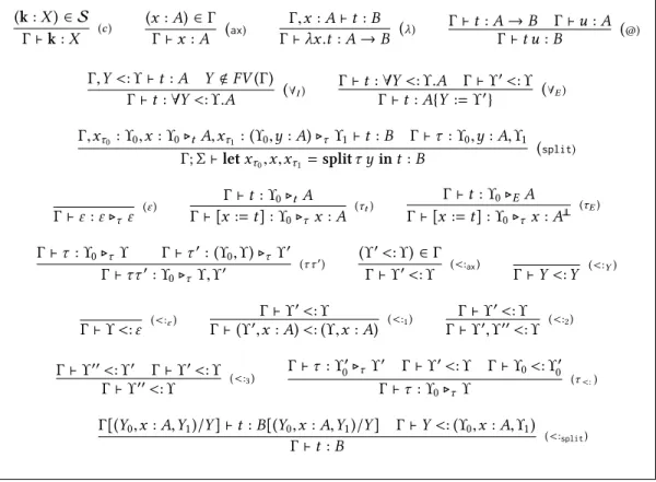
2 THE λ[lvτ ⋆]-CALCULUS SYNTAX

2.1 Syntax

While all the results that are presented in the sequel of this paper could be directly expressed using

theλ_lv-calculus, the continuation-passing-style translation we present naturally arises from the decomposition of this calculus into a different calculus with an explicitenvironment, the λ[lvτ ⋆]

-calculus [2]. Indeed, as we shall explain thereafter, the decomposition highlights different syntactic

5

⟨t || ˜µx .c⟩τ → cτ [x := t] ⟨µα .c ||E⟩τ → cτ [α := E] ⟨V ||α ⟩τ [α := E]τ′ → ⟨V ||E⟩τ [α := E]τ′

⟨x ||F ⟩τ [x := t]τ′ → ⟨t || ˜µ[x].⟨x ||F ⟩τ′⟩τ ⟨V || ˜µ[x].⟨x ||F ⟩τ′⟩τ → ⟨V ||F ⟩τ [x := V ]τ′ ⟨λx .t ||u · E⟩τ → ⟨u || ˜µx .⟨t ||E⟩⟩τ

Fig. 2. Reduction rules of the λ[lvτ ⋆]-calculus

categories that are deeply involved in the definition and the typing of the continuation-passing-style

translation.

The explicit environment ofλ[lvτ ⋆]-calculus, also calledsubstitution or store, binds terms which

are lazily evaluated. The reduction system resembles the one of an abstract machine.

Note that our approach slightly differ from [2] in that we split values into two categories: strong

values (v) and weak values (V ). The strong values correspond to values stricly speaking. The weak values include the variables which force the evaluation of terms to which they refer into shared

strong value. Their evaluation may require capturing a continuation.

Besides, we reformulate the construction ˜µx .C[⟨x ||F ⟩] of λ_lv into ˜µ[x].⟨x ||F ⟩τ . It expresses the fact that the variablex is forced at top-level. The syntax of the language is given by:

Strong values v ::= λx.t | k Weak values V ::= v | x Terms t ,u ::= V | µα.c Forcing contexts F ::= t · E | κ | Catchable contexts E ::= F | α | ˜µ[x].⟨x||F⟩τ Evaluation contexts e ::= E | ˜µx.c Stores τ ::= ε | τ [x := t] | τ [α := E] Commands c ::= ⟨t ||e⟩ Closures l ::= cτ

and the reduction, written→, is the compatible reflexive transitive closure of the rules given in Figure2. The different syntactic categories can be understood as the different levels of alternation in a context-free abstract machine [2]: the priority is first given to contexts at levele (lazy storage of terms), then to terms at levelt (evaluation of µα into values), then back to contexts at level E and so on until levelv. These different categories are directly reflected in the definition of the continuation-passing-style translation, and thus involved when typing it. We chose to highlight

this by distinguishing different types of sequents already in the typing rules that we shall now

present.

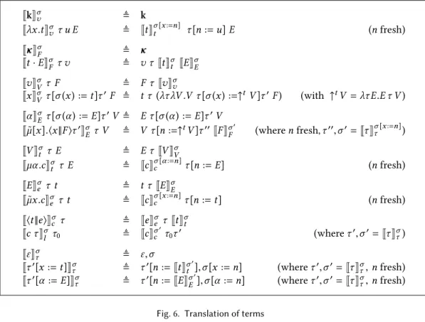
2.2 A type system for the λ[lvτ ⋆]-calculus.

Unlike in the usual type system for sequent calculus where, as in the previous section, a judgment

contains two typing contexts (one on the left for proofs, denoted byΓ, one on the right for contexts denoted by∆), we group both of them into one single context, denoting the types for contexts (that used to be in∆) with the exponent ⊥⊥. This allows to draw a strong connection in the sequel between the typing contextsΓ and the store τ , which contains both kind of terms.

We have nine kinds of sequents, one for typing each of the nine syntactic categories. We write

them with an annotation on the⊢ sign, using one of the lettersv, V , t , F , E, e, l, c, τ . Sequents themselves are of four sorts: those typing values and terms are asserting a type, with the type

(k : X ) ∈ S Γ ⊢vk : X (k) Γ,x : A ⊢t t : B Γ ⊢v λx .t : A → B (→r) (x : A) ∈ Γ Γ ⊢V x : A (x ) Γ ⊢vv : A Γ ⊢V v : A (↑V) (κ : A) ∈ S Γ ⊢F κ : A⊥⊥ (κ ) Γ ⊢tt : A Γ ⊢E E : B ⊥ ⊥ Γ ⊢F t · E :(A → B)⊥⊥ (→l) (α : A) ∈ Γ Γ ⊢E α : A⊥⊥ (α ) Γ ⊢F F : A⊥⊥ Γ ⊢E F : A⊥ (⊥ ↑ E₎ Γ ⊢V V : A Γ ⊢tV : A (↑ t₎ Γ,α : A ⊥ ⊥_⊢ cc Γ ⊢t µα .c : A (µ) Γ ⊢E E : A⊥⊥ Γ ⊢e E : A⊥⊥ (↑ e₎ Γ,x : A ⊢cc Γ ⊢e µx .c : A˜ ⊥⊥ ( ˜µ) Γ,x : A, Γ′_⊢ F F : A⊥⊥ _{Γ ⊢} τ τ :Γ′ Γ ⊢E µ[x].⟨x ||F ⟩τ : A˜ ⊥⊥ ( ˜µ[]₎ Γ ⊢tt : A Γ ⊢ee : A ⊥ ⊥ Γ ⊢c ⟨t ||e⟩ (c ) Γ, Γ′_⊢ cc Γ ⊢τ τ :Γ′ Γ ⊢l cτ (l ) Γ ⊢τ ε : ε (ε ) Γ ⊢ττ :Γ′ Γ, Γ′⊢_t t : A Γ ⊢τ τ [x := t] : Γ′,x : A (τt) Γ ⊢τ τ :Γ′ Γ, Γ′⊢_E E : A⊥⊥ Γ ⊢τ τ [α := E] : Γ′,α : A⊥⊥ (τE)

Fig. 3. Typing rules of the λ[lvτ ⋆]-calculus

sequents typing commands and closures are black boxes neither asserting nor expecting a type;

sequents typing substitutions are instantiating a typing context. In other words, we have the

following nine kinds of sequents: Γ ⊢l l Γ ⊢cc Γ ⊢τ τ :Γ′ Γ ⊢tt : A Γ ⊢V V : A Γ ⊢vv : A Γ ⊢e e : A⊥⊥ Γ ⊢E E : A⊥⊥ Γ ⊢F F : A⊥⊥

where types and typing contexts are defined by:

A, B ::= X | A → B Γ ::= ε | Γ,x : A | Γ,α : A⊥⊥

The typing rules are given on Figure3where we assume that a variablex (resp. co-variable α ) only occurs once in a contextΓ (we implicitly assume the possibility of renaming variables by α -conversion). This type system enjoys the property of subject reduction.

Theorem 2.1 (Subject reduction). IfΓ ⊢_l cτ and cτ → c′τ′thenΓ ⊢_lc′τ′.

3 NORMALIZATION OF THEλ[lvτ ⋆]-CALCULUS

3.1 Normalization by realizability

The proof of normalization for theλ_{[lvτ ⋆]}-calculus that we present in this section is inspired from techniques of Krivine’s classical realizability [17], whose notations we borrow. Actually, it is also

very close to a proof by reducibility6. In a nutshell, to each typeA is associated a set |A|_t of terms whose execution is guided by the structure ofA. These terms are the one usually called realizers in Krivine’s classical realizability. Their definition is in fact indirect, and is done by orthogonality

to a set of “correct” computations, called apole. The choice of this set is central when studying models induced by classical realizability for second-order-logic, but in the present case we only pay

attention to the particular pole of terminating computations. This is where sites the main difference

with a proof by reducibility, where everything is done with respect toSN , while our definition are 6

parametric in the pole (which is chosen to beSN in the end). The adequacy lemma, which is the central piece, consists in proving that typed terms belongs to the corresponding sets of realizers,

and are thus normalizing.

More in details, our proof can be sketched as follows. First, we generalize the usual notion of

closed term to the notion of closedterm-in-store. Intuitively, this is due to the fact that we are no longer interested in closed terms and substitutions to close open terms, but rather in terms that

are closed when considered in the current store. This is based on the simple observation that a

store is nothing more than a shared substitution whose content might evolve along the execution.

Second, we define the notion ofpole ⊥⊥, which are sets of closures closed by anti-evaluation and store extension. In particular, the set of normalizing closures is a valid pole. This allows to relate

terms and contexts thanks to a notion of orthogonality with respect to the pole. We then define for

each formulaA and typing level o (of e,t , E,V , F ,v) a set |A|_o (resp.∥A∥_o) of terms (resp. contexts) in the corresponding syntactic category. These sets correspond to reducibility candidates, or to

what is usually called truth values and falsity values in realizability. Finally, the core of the proof

consists in the adequacy lemma, which shows that any closed term of typeA at level o is in the corresponding set|A|_o. This guarantees that any typed closure is in any pole, and in particular in the pole of normalizing closures. Technically, the proof of adequacy evaluates in each case a

state of an abstract machine (in our case a closure), so that the proof also proceeds by evaluation.

A more detailed explanation of this observation as well as a more introductory presentation of

normalization proofs by classical realizability are given in an article by Dagand and Scherer [8].

3.2 Realizability interpretation for the λ[lvτ ⋆]-calculus

We begin by defining some key notions for stores that we shall need further in the proof.

Definition 3.1 (Closed store). We extend the notion of free variable to stores: FV(ε) ≜ ∅

FV(τ [x := t]) ≜ FV (τ ) ∪ {y ∈ FV (t) : y < dom(τ )} FV(τ [α := E]) ≜ FV (τ ) ∪ {β ∈ FV (E) : β < dom(τ )} so that we can define aclosed store to be a store τ such that FV(τ ) = ∅.

Definition 3.2 (Compatible stores). We say that two stores τ and τ′_{areindependent and note}

τ # τ′_{whendom(τ ) ∩ dom(τ}′_{) = ∅. We say that they are compatible and note τ <:τ}′_{whenever for all}

variablesx (resp. co-variables α ) present in both stores: x ∈ dom(τ ) ∩ dom(τ′); the corresponding terms (resp. contexts) inτ and τ′coincide: formallyτ = τ0[x := t]τ1andτ

′_{= τ}′

0[x := t]τ ′

1. Finally,

we say thatτ′is anextension of τ and note τ ◁ τ′wheneverdom(τ ) ⊆ dom(τ′) and τ <: τ′. We denote byττ′the compatible unionjoin(τ ,τ′) of closed stores τ and τ′, defined by:

join(τ0[x := t]τ1,τ ′ 0[x := t]τ ′ 1) ≜ τ0τ ′ 0[x := t]join(τ1,τ ′ 1) join(τ ,τ′) ≜ ττ′ join(ε,τ ) ≜ τ join(τ ,ε) ≜ τ (if τ0#τ ′ 0) (if τ # τ′₎

The following lemma (which follows easily from the previous definition) states the main property

we will use about union of compatible stores.

Lemma 3.3. If τ and τ′are two compatible stores, then τ ◁ ττ′and τ′◁ ττ′. Besides, if τ is of the form τ0[x := t]τ1, then ττ′is of the form τ0[x := t]τ1with τ0◁ τ0and τ1◁ τ1.

As we explained in the introduction of this section, we will not consider closed terms in the usual

of a calculus to consider only closed terms and to perform substitutions to maintain the closure

of terms, this only makes sense if it corresponds to the computational behavior of the calculus.

For instance, to prove the normalization ofλx .t in typed call-by-name λµ ˜µ-calculus, one would consider a substitutionρ that is suitable for with respect to the typing contextΓ, then a context u · e of type A → B, and evaluates :

⟨λx .tρ||u · e⟩ → ⟨tρ[u/x]||e⟩

Then we would observe thatt_ρ[u/x]= t_ρ[x:=u]and deduce thatρ[x := u] is suitable for Γ,x : A, which would allow us to conclude by induction.

However, in theλ[lvτ ⋆]-calculus we do not perform global substitution when reducing a command,

but rather add a new binding [x := u] in the store:

⟨λx .t ||u · E⟩τ → ⟨t ||E⟩τ [x := u]

Therefore the natural notion of closed term invokes the closure under a store, which might evolve

during the rest of the execution (this is to contrast with a substitution).

Definition 3.4 (Term-in-store). We call closed term-in-store (resp. closed context-in-store, closed closures) the combination of a term t (resp. context e, command c) with a closed store τ such that FV(t ) ⊆ dom(τ ). We use the notation (t |τ ) to denote such a pair.

We should note that in particular, ift is a closed term, then(t |τ ) is a term-in-store for any closed storeτ . The notion of closed term-in-store is thus a generalization of the notion of closed terms, and we will (ab)use of this terminology in the sequel. We denote the sets of closed closures byC0,

and will identify(c|τ ) and the closure cτ when c is closed in τ . Observe that if cτ is a closure in C0

andτ′is a store extendingτ , then cτ′is also inC0. We are now equipped to define the notion of

pole, and verify that the set of normalizing closures is indeed a valid pole.

Definition 3.5 (Pole). A subset ⊥⊥ ∈ C0is said to besaturated or closed by anti-reduction whenever

for all(c|τ ), (c′|τ′) ∈ C0, ifc ′

τ′ ∈ ⊥⊥ andcτ → c′τ′thencτ ∈ ⊥⊥. It is said to beclosed by store extension if whenever cτ ∈ ⊥⊥, for any storeτ′extendingτ : τ ◁ τ′,cτ′∈ ⊥⊥. Apole is defined as any subset ofC0that is closed by anti-reduction and store extension.

The following proposition is the one supporting the claim that our realizability proof is almost a

reducibility proof whose definitions have been generalized with respect to a pole instead of the

fixed set SN.

Proposition 3.6. The set ⊥⊥_⇓= {cτ ∈ C0: cτ normalizes } is a pole.

Proof. As we only considered closures inC0, both conditions (closure by anti-reduction and

store extension) are clearly satisfied:

• ifcτ → c′_τ′_andc′_τ′_{normalizes, thencτ normalizes too;}

• if_{c is closed in τ and cτ normalizes, if τ ◁ τ}′_thencτ′_{will reduce ascτ does (since c is}

closed underτ , it can only use terms in τ′that already were inτ ) and thus will normalize. □ Definition 3.7 (Orthogonality). Given a pole ⊥⊥, we say that a term-in-store(t |τ ) is orthogonal to a context-in-store(e|τ′) and write (t |τ )⊥⊥(e|τ′) if τ and τ′are compatible and⟨t ||e⟩ττ′∈ ⊥⊥.

We can now relate closed terms and contexts by orthogonality with respect to a given pole. This

allows us to define for any formulaA the sets |A|_v, |A|_V, |A|_t(resp.∥A∥_F,∥A∥_E,∥A∥_e) of realizers (or reducibility candidates) at levelv, V , t (resp F , E, e) for the formula A. It is to be observed that realizers are here closed terms-in-store.

Definition 3.8 (Realizers). Given a fixed pole ⊥⊥, we set: |X |v = {(k|τ ) : ⊢ k : X }

|A → B|v = {(λx.t |τ ) : ∀uτ′,τ <: τ′∧(u|τ′) ∈ |A|_t ⇒(t |ττ′_{[x := u]) ∈ |B|} t} ∥A∥F = {(F |τ ) : ∀vτ′,τ <: τ′∧(v|τ′) ∈ |A|_v⇒(v|τ′)⊥⊥(F |τ )}

|A|V = {(V |τ ) : ∀Fτ′,τ <: τ′∧(F |τ′) ∈ ∥A∥F ⇒(V |τ )⊥⊥(F |τ′)}

∥A∥E = {(E|τ ) : ∀Vτ′,τ <: τ′∧(V |τ′) ∈ |A|V ⇒(V |τ′)⊥⊥(E|τ )}

|A|t = {(t |τ ) : ∀Eτ′,τ <: τ′∧(E|τ′_{) ∈ ∥A∥}

E ⇒(t |τ )⊥⊥(E|τ′_)}

∥A∥e = {(e|τ ) : ∀tτ′,τ <: τ′∧(t |τ′_{) ∈ |A|}

t ⇒(t |τ′_{)⊥⊥(e|τ )}}

Remark 3.9. We draw the reader attention to the fact that we should actually write |A|_v⊥⊥, ∥A∥⊥⊥

F ,

etc... and τ ⊩⊥⊥Γ, because the corresponding definitions are parameterized by a pole ⊥⊥. As it is common

in Krivine’s classical realizability, we ease the notations by removing the annotation ⊥⊥whenever there is no ambiguity on the pole.

If the definition of the different sets might seem complex at first sight, we claim that they are

quite natural in regards of the methodology of Danvy’s semantics artifacts presented in [2]. Indeed,

having an abstract machine in context-free form (the last step in this methodology before deriving

the CPS) allows us to have both the term and the context (in a command) that behave independently

of each other. Intuitively, a realizer at a given level is precisely a term which is going to behave well

(be in the pole) in front of any opponent chosen in the previous level (in the hierarchyv, F ,V ,etc...). For instance, in a call-by-value setting, there are only three levels of definition (values, contexts

and terms) in the interpretation, because the abstract machine in context-free form also has three.

Here the ground level corresponds to strong values, and the other levels are somewhat defined

as terms (or context) which are well-behaved in front of any opponent in the previous one. The

definition of the different sets|A|_v, ∥A∥_F, |A|_V, etc... directly stems from this intuition.

In comparison with the usual definition of Krivine’s classical realizability, we only considered

orthogonal sets restricted to some syntactical subcategories. However, the definition still satisfies

the usual monotonicity properties of bi-orthogonal sets:

Proposition 3.10. For any type A and any given pole ⊥⊥, we have the following inclusions (1) |A|_v ⊆ |A|_V ⊆ |A|_t;

(2) ∥A∥_F ⊆ ∥A∥_E ⊆ ∥A∥_e.

Proof. All the inclusions are proved in a similar way. We only give the proof for|A|_v ⊆ |A|_V. Let⊥⊥ be a pole and(v|τ ) be in |A|_v. We want to show that(v|τ ) is in |A|_V, that is to say that v is in the syntactic category V (which is true), and that for any(F |τ′_{) ∈ ∥A∥}

F such thatτ <: τ′, (v|τ )⊥⊥(F |τ′_{). The latter holds by definition of (F |τ}′_{) ∈ ∥A∥}

F, since(v|τ ) ∈ |A|_v. □ We now extend the notion of realizers to stores, by stating that a storeτ realizes a contextΓ if it binds all the variablesx and α inΓ to a realizer of the corresponding formula.

Definition 3.11. Given a closed store τ and a fixed pole ⊥⊥, we say thatτ realizesΓ and write τ ⊩ Γ if:

(1) for any(x : A) ∈ Γ, τ ≡ τ0[x := t]τ1and(t |τ0) ∈ |A|t

(2) for any(α : A⊥⊥) ∈ Γ, τ ≡ τ0[α := E]τ1and(E|τ0) ∈ ∥A∥E

In the same way as weakening rules (for the typing context) were admissible for each level of

the typing system :

Γ ⊢tt : A Γ ⊆ Γ′ Γ′_⊢ t t : A Γ ⊢ee : A⊥⊥ Γ ⊆ Γ′ Γ′_⊢ ee : A⊥⊥ . . . Γ ⊢ττ :Γ′′ Γ ⊆ Γ′ Γ′_⊢ τ τ :Γ′′

the definition of realizers is compatible with a weakening of the store.

Lemma 3.12 (Store weakening). Let τ and τ′be two stores such that τ ◁ τ′,Γ be a typing context and let ⊥⊥be a pole. The following holds:

(1) If(t |τ ) ∈ |A|_t for some closed term(t |τ ) and type A, then (t |τ′) ∈ |A|_t. The same holds for each level e, E,V , F ,v of the typing rules.

(2) If τ ⊩ Γ then τ′⊩ Γ. Proof.

(1) This essentially amounts to the following observations. First, one remarks that if(t |τ ) is a closed term, so is(t |ττ′) for any store τ′compatible withτ . Second, we observe that if we consider for instance a closed context(E|τ′′) ∈ ∥A∥_E, thenττ′<: τ′′impliesτ <: τ′′, thus (t |τ )⊥⊥(E|τ′′_{) and finally (t |ττ}′_)⊥⊥(E|τ′′_{) by closure of the pole under store extension. We}

conclude that(t |τ′)⊥⊥(E|τ′′) using the first statement.

(2) By definition, for all(x : A) ∈ Γ, τ is of the form τ0[x := t]τ1such that(t |τ0) ∈ |A|t. Asτ

andτ′are compatible, we know by Lemma3.3thatττ′is of the formτ′

0[x := t]τ ′ 1withτ

′ 0

an extension ofτ0, and using the first point we get that(t |τ ′

0) ∈ |A|t. □

Definition 3.13 (Adequacy). Given a fixed pole ⊥⊥, we say that:

• A typing judgmentΓ ⊢_t t : A is adequate (w.r.t. the pole ⊥⊥) if for all stores_{τ ⊩ Γ, we have} (t |τ ) ∈ |A|t.

• More generally, we say that an inference rule J1 · · · Jn

J0

is adequate (w.r.t. the pole⊥⊥) if the adequacy of all typing judgmentsJ1, . . . , Jnimplies the

adequacy of the typing judgmentJ0.

Remark 3.14. From the latter definition, it is clear that a typing judgment that is derivable from a set of adequate inference rules is adequate too.

Lemma 3.15 (Adeqacy). The typing rules of Figure3for the λ_{[lvτ ⋆]}-calculus without co-constants are adequate with any pole.

Proof. We proceed by induction over the typing rules. The exhaustive induction is given in

AppendixB, we only give some two cases here to give an idea of the proof Rule(→l). Assume that

Γ ⊢tu : A Γ ⊢E E : B⊥⊥

Γ ⊢F u · E :(A → B)⊥⊥ (→l)

and let⊥⊥ be a pole andτ a store such that τ ⊩ Γ. Let (λx .t |τ′) be a closed term in the set |A → B|_v such thatτ <: τ′, then we have:

⟨λx .t ||u · E⟩ττ′ _{→ ⟨u || ˜µx .⟨t ||E⟩⟩ττ}′ _{→ ⟨t ||E⟩ττ}′_[x := u]

By definition of|A → B|_v, this closure is in the pole, and we can conclude by anti-reduction. Rule( ˜µ[]). Assume that

Γ,x : A, Γ′_⊢

F F : A Γ,x : A ⊢ τ′:Γ′ Γ ⊢E µ[x].⟨x ||F ⟩τ˜ ′:A

and let⊥⊥ be a pole andτ a store such that τ ⊩ Γ. Let (V |τ0) be a closed term in |A|V such that

τ0<: τ . We have that :

⟨V || ˜µ[x].⟨x ||F ⟩τ′_⟩τ

0τ → ⟨V ||F ⟩τ0τ [x := V ]τ ′

By induction hypothesis, we obtainτ [x := V ]τ′⊩ Γ,x : A, Γ′. Up toα -conversion in F and τ′, so that the variables inτ′are disjoint from those inτ₀, we have thatτ₀τ ⊩ Γ (by Lemma3.12) and then τ′′≜ τ0τ [x := V ]τ

′

⊩ Γ,x : A, Γ′. By induction hypothesis again, we obtain that(F |τ′′) ∈ ∥A∥_F (this was an assumption in the previous case) and as(V |τ0) ∈ |A|V, we finally get that(V |τ0)⊥⊥(F |τ

′′₎

and conclude again by anti-reduction.

□ The previous result required to consider theλ[lvτ ⋆]-calculus without co-constants. Indeed, we

consider co-constants as coming with their typing rules, potentially giving them any type (whereas

constants can only be given an atomic type). Thus there isa priori no reason7why their types should be adequate with any pole.

However, as observed in the previous remark, given a fixed pole it suffices to check whether the

typing rules for a given co-constant are adequate with this pole. If they are, any judgment that is

derivable using these rules will be adequate.

Corollary 3.16. If cτ is a closure such that ⊢_l cτ is derivable, then for any pole ⊥⊥such that the typing rules for co-constants used in the derivation are adequate with ⊥⊥, cτ ∈ ⊥⊥.

We can now put our focus back on the normalization of typed closures. As we already saw in

Proposition3.6, the set⊥⊥_⇓of normalizing closure is a valid pole, so that it only remains to prove that any typing rule for co-constants is adequate with⊥⊥_⇓. This proposition directly stems from the observation that for any storeτ and any closed strong value(v|τ′) ∈ |A|_v,⟨v ||κ⟩ττ′does not reduce and thus belongs to the pole⊥⊥_⇓.

Lemma 3.17. Any typing rule for co-constants is adequate with the pole ⊥⊥_⇓, i.e. ifΓ is a typing context, and τ is a store such that τ ⊩ Γ, if κ is a co-constant such that Γ ⊢F κ : A⊥⊥, then(κ |τ ) ∈ ∥A∥F.

As a consequence, we obtain the normalization of typed closures of the full calculus.

Theorem 3.18. If cτ is a closure of the λ_{[lvτ ⋆]}-calculus such that ⊢_l cτ is derivable, then cτ normalizes.

Besides, the translations8fromλ_lvtoλ[lvτ ⋆]defined by Ariolaet al. both preserve normalization

[2, Theorem 2,4]. As it is clear that they also preserve typing, the previous result also implies the

normalization of theλ_lv-calculus:

Corollary 3.19. If c is a closure of the λ_lv-calculus such that c : ( ⊢ ) is derivable, then c normalizes. This is to be contrasted with Okasaki, Lee and Tarditi’s semantics for the call-by-needλ-calculus, which is not normalizing in the simply-typed case, as shown in Ariolaet al [2].

4 A TYPED STORE-AND-CONTINUATION-PASSING STYLE TRANSLATION

Guided by the normalization proof of the previous section, we shall now present a type system

adapted to the continuation-passing style translation defined in [2]. The computational part is

almost the same, except for the fact that we explicitly handle renaming through a substitutionσ that replaces names of the source language by names of the target.

7

Think for instance of a co-constant of type(A → B)⊥⊥, there is no reason why it should be orthogonal to any function in |A → B |v.

8

4.1 Guidelines of the translation

The transformation is actually not only a continuation-passing style translation. Because of the

sharing of the evaluation of arguments, the environment associating terms to variables behaves

like a store which is passed around. Passing the store amounts to combine the continuation-passing

style translation with a store-passing style translation. Additionally, the store is extensible, so, to

anticipate extension of the store, Kripke style forcing has to be used too, in a way comparable to

what is done in step-indexing translations. Before presenting in detail the target system of the

translation, let us explain step by step the rationale guiding the definition of the translation. To

facilitate the comprehension of the different steps, we illustrate each of them with the translation

of the sequenta : A,α : A⊥⊥,b : B ⊢_e e : C.

Step 1 - Continuation-passing style. In a first approximation, let us look only at the continuation-passing style part of the translation of aλ_{[lvτ ⋆]}sequent.

As shown in [2] and as emphasized by the definition of realizers (see Definition3.8) reflecting the 6 nested syntactic categories used to defineλ[lvτ ⋆], there are 6 different levels of control in

call-by-need, leading to 6 mutually defined levels of interpretation. We define

JA→BKvfor strong values as

JAKt →JBKE, we defineJAKF for forcing contexts as¬JAKv,JAKV for weak values as ¬

JAKF =

2

¬

JAKv, and so on untilJAKedefined as

5 ¬ JAKv(where 0 ¬ A ≜ A andn+1 ¬ A ≜ ¬ n ¬ A). As we already observed in the previous section (see Definition3.11), hypothesis from a context Γ of the form α : A⊥⊥_{are to be translated as}

JAKE =

3

¬

JAKvwhile hypothesis of the formx : A are to be translated as

JAKt =

4

¬

JAKv. Up to this point, if we denote this translation ofΓ byJΓK, in the particular case ofΓ ⊢_t A the translation is

JΓK ⊢ JAKt and similarly for other levels,e.g.Γ ⊢e A translates to

JΓK⊢JAKe.

Example 4.1 (Translation, step 1). Up to now, the translation taking into account the continuation-passing style ofa : A,α : A⊥⊥,b : B ⊢_ee : C is simply:

Ja:A,α : A ⊥ ⊥_{,b : B ⊢} ee : CK = a :JAKt ,α :JAKE ,b :JBKt ⊢Je Ke :JC Ke = a :_¬4 JAKv ,α : 3 ¬ JAKv,b : 4 ¬ JBKv⊢Je Ke : 5 ¬ JC Kv

Step 2 - Store-passing style. The continuation-passing style part being settled, the store-passing style part should be considered. In particular, the translation ofΓ ⊢_t A is not anymore a sequent JΓK⊢JAKt but instead a sequent roughly of the form⊢JΓK→JAKt, with actuallyJΓKbeing passed around not only at the top level of

JAKtbut also every time a negation is used. We write this sequent ⊢_{JΓK ▷t}A where ▷tA is defined by induction on t and A, with

JΓK ▷tA=JΓK→(JΓK ▷EA) → ⊥

=JΓK→(JΓK→ (JΓK ▷VA) → ⊥) → ⊥ = . . .

Moreover, the translation of each type inΓ should itself be abstracted over the store at each use of a negation.

Example 4.2 (Translation, step 2). Up to now, the continuation-and-store passing style translation ofa : A,α : A⊥⊥,b : B ⊢_ee : C is: Ja:A,α : A ⊥ ⊥_{,b : B ⊢} ee : CK =⊢Je K σ e : Ja:A,α : A ⊥ ⊥_{,b : B} K ▷eC = ⊢Je K σ e : Ja:A,α : A ⊥ ⊥_{,b : BK} →(Ja:A,α : A⊥⊥,b : BK ▷_tC) → ⊥ = ... where: Ja:A,α : A ⊥ ⊥_{,b : B} K =Ja:A,α : A ⊥ ⊥ K, b:Ja:A,α : A ⊥ ⊥ K ▷tB =Ja:A,α : A ⊥ ⊥ K, b:Ja:A,α : A ⊥ ⊥ K→(Ja:A,α : A ⊥ ⊥ K ▷EB) → ⊥ = ...

and: Ja:A,α : A ⊥ ⊥ K =Ja:AK, α:Ja:AK ▷EA =Ja:AK, α:Ja:AK→(Ja:AK→▷EA) → ⊥ = ... Ja:AK = a : ε ▷tA = a : 4 ¬ JAKv

Step 3 - Extension of the store. The store-passing style part being settled, it remains to anticipate that the store is extensible. This is done by supporting arbitrary insertions of any term at any

place of the store. The extensibility is obtained by quantification over all possible extensions of

the store at each level of the negation. This corresponds to the intuition that in the realizability

interpretation, given a sequentΓ ⊢_tt : A we showed that for any store τ such that τ ⊩ Γ, we had (t |τ ) in |A|t. But the definition ofτ ⊩ Γ is such that for any Γ′ ⊇Γ, if τ ⊩ Γ′thenτ ⊩ Γ, so that actually(t |τ′) is also |A|_t. The termt was thus compatible with any extension of the store.

For this purpose, we use as type system an adaptation of SystemF_<:[5] extended with stores, defined as lists of assignations [x := t]. Store types, denoted by ϒ, are defined as list of types of the form(x : A) where x is a name and A is a type properly speaking and admit a subtyping notion ϒ′_{<: ϒ to express that ϒ}′_{is an extension ofϒ. This corresponds to the following refinement of the}

definition of JΓK ▷tA: JΓK ▷tA = ∀ϒ <:JΓK.ϒ→ (ϒ ▷EA) → ⊥ = ∀ϒ <:JΓK.ϒ→ (∀ϒ ′_{<: ϒ.ϒ}′_→ϒ′_▷ VA → ⊥) → ⊥ = ...

The reader can think of subtyping as a sort of Kripke forcing [15], whereworlds are store typesϒ andaccessible worlds fromϒ are precisely all the possible ϒ′<: ϒ.

Example 4.3 (Translation, step 3). The translation, now taking into account store extensions, of a : A,α : A⊥⊥,b : B ⊢ee : C becomes: Ja:A,α : A ⊥ ⊥_{,b : B ⊢} e e : CK = ⊢Je K σ e : Ja:A,α : A ⊥ ⊥_{,b : B} K ▷eC = ⊢Je K σ e :∀ϒ <: Ja:A,α : A ⊥ ⊥_{,b : B} K.ϒ→(ϒ ▷tC) → ⊥ = ... where: Ja:A,α : A ⊥ ⊥_{,b : B} K = Ja:A,α : A ⊥ ⊥ K, b :Ja:A,α : A ⊥ ⊥ K ▷tB = Ja:A,α : A ⊥ ⊥ K, b :∀ϒ <:Ja:A,α : A ⊥ ⊥ K.ϒ→(ϒ ▷EB) → ⊥ = ... Ja:A,α : A ⊥ ⊥ K = Ja:AK, α:Ja:AK ▷EA = Ja:AK, α:∀ϒ <:Ja:AK.ϒ→(ϒ → ▷EA) → ⊥ = ... Ja:AK = a : ε ▷tA = a : ∀ϒ.ϒ → (ϒ ▷EA) → ⊥

Step 4 - Explicit renaming. As we will explain in details in the next section (see Section5.1), we need to handle the problem of renaming the variables during the translation. We assume that we

dispose of a generator of fresh names (in the target language). In practice, this means that the

implementation of the CPS requires for instance to have a list keeping tracks of the variables already

used. In the case where variable names can be reduced to natural numbers, this can be easily done

with a reference that is incremented each time a fresh variable is needed. The translation is thus

annotated by a substitutionσ which binds names from the source language with names in the target language. For instance, the translation of a typing contexta : A,α : A⊥⊥,b : B is now:

Ja:A,α : A ⊥ ⊥_{,b : B} K σ _{= σ (a) : ε ▷tA, σ(α ) :} Ja:AK σ _{▷EA, σ(b) :} Ja:A,α : A ⊥ ⊥ K σ _▷tB

4.2 The target language: System Fϒ

The target language is thus the usualλ-calculus extended with stores (defined lists of pairs of a name and a term) and second-order quantification over store types. We refer to this language as

(k : X ) ∈ S Γ ⊢ k : X (c ) (x : A) ∈ Γ Γ ⊢ x : A (ax) Γ,x : A ⊢ t : B Γ ⊢ λx.t : A → B (λ) Γ ⊢ t : A → B Γ ⊢ u : AΓ ⊢ t u : B (@) Γ,Y <: ϒ ⊢ t : A Y < FV (Γ)

Γ ⊢ t : ∀Y <: ϒ.A (∀I) Γ ⊢ t : ∀Y <: ϒ.A Γ ⊢ ϒ

′_{<: ϒ} Γ ⊢ t : A{Y := ϒ′_} (∀E) Γ,xτ0 :ϒ0,x : ϒ0▷tA,xτ1:(ϒ0,y : A) ▷τϒ1⊢t : B Γ ⊢ τ : ϒ0,y : A,ϒ1 Γ; Σ ⊢ let xτ0,x,xτ1 = splitτ y in t : B (split) Γ ⊢ ε : ε ▷τ ε (ε ) Γ ⊢ t : ϒ0▷tA Γ ⊢ [x := t] : ϒ0▷τ x : A (τt) Γ ⊢ t : ϒ 0▷EA Γ ⊢ [x := t] : ϒ0▷τx : A ⊥ ⊥ (τE) Γ ⊢ τ : ϒ0▷τ ϒ Γ ⊢ τ ′_:(ϒ 0,ϒ) ▷τ ϒ ′ Γ ⊢ ττ′_:ϒ 0▷τ ϒ,ϒ ′ (τ τ′) (ϒ′_{<: ϒ) ∈ Γ} Γ ⊢ ϒ′_{<: ϒ} (<:ax) Γ ⊢ Y <: Y (<:Y) Γ ⊢ ϒ <: ε (<:ε) Γ ⊢ ϒ ′_{<: ϒ} Γ ⊢ (ϒ′_{,x : A) <: (ϒ,x : A)} (<:1) Γ ⊢ ϒ′_{<: ϒ} Γ ⊢ ϒ′_,ϒ′′_{<: ϒ} (<:2) Γ ⊢ ϒ′′_{<: ϒ}′ _{Γ ⊢ ϒ}′_{<: ϒ} Γ ⊢ ϒ′′_{<: ϒ} (<:3) Γ ⊢ τ : ϒ′ 0▷τ ϒ ′ _{Γ ⊢ ϒ}′_{<: ϒ Γ ⊢ ϒ} 0<: ϒ ′ 0 Γ ⊢ τ : ϒ0▷τ ϒ (τ<:)

Γ[(Y0,x : A,Y1)/Y ] ⊢ t : B[(Y0,x : A,Y1)/Y ] Γ ⊢ Y <: (ϒ0,x : A,ϒ1)

Γ ⊢ t : B (<:split)

Fig. 4. Typing rules of System F_ϒ

system, and we still denote this constant byX . This allows us to define an embedding ι from the original type system to this one by:

ι(X ) = X ι(A → B) = ι(A) → ι(B). The syntax for terms and types is given by:

t ,u ::= k | x | λx.t | tu | τ |let xτ0,x,xτ1 = splitτ ′′_{y in t} τ ,τ′_{::= ε | τ [x := t]} A, B ::= X | ⊥ | ϒ ▷τ ϒ′|A → B | ∀Y <:ϒ. A ϒ,ϒ′_{::= ε | (x : A) | (x : A}⊥⊥_{) | Y | ϒ,ϒ}′ Γ, Γ′_{::= ε | Γ,x : A | Γ,Y <: ϒ}

We introduce a new symbolϒ ▷_τ ϒ′to denote the fact that a store has a type conditioned byϒ (which should be the type of the head of the list). In order to ease the notations, we will denote ϒ instead of ε ▷τϒ in the sequel. On the contrary, ϒ ▷tA is a shorthand (defined in Figure5). The type system is given in Figure4where we assume that a name can only occur once both in typing contextsΓ and stores types ϒ.

Remark 4.4. We shall make a few remarks about our choice of rules for typing stores. First, observe that we force elements of the store to have types of the formϒ ▷tA, that is having the structure of

types obtained through the CPS translation. Even though this could appear as a strong requirement, it appears naturally when giving a computational contents to the inclusionϒ′_{<: ϒ with De Bruijn levels}

(see Section5.3). Indeed, a De Bruijn level (just as a name) can be understood as a pointer to a particular cell of the store. Therefore, we need to update pointers when inserting a new element. Such an operation

JΓ⊢ee : A ⊥ ⊥ K ≜ ∀σ , σ s Γ ⇒ (⊢ Je K σ e : JΓK σ Γ ▷eι(A)) JΓ⊢tt : AK ≜ ∀σ , σ s Γ ⇒ (⊢ Jt K σ t : JΓK σ Γ ▷tι(A)) JΓ⊢E E : A ⊥ ⊥ K ≜ ∀σ , σ s Γ ⇒ (⊢ JE K σ E: JΓK σ Γ ▷Eι(A)) JΓ⊢VV : AK ≜ ∀σ , σ s Γ ⇒ (⊢ JV K σ V: JΓK σ Γ ▷Vι(A)) JΓ⊢F F : A ⊥ ⊥ K ≜ ∀σ , σ s Γ ⇒ (⊢ JF K σ F : JΓK σ Γ ▷F ι(A)) JΓ⊢vv : AK ≜ ∀σ , σ s Γ ⇒ (⊢ Jv K σ v: JΓK σ Γ ▷vι(A)) JΓ⊢ccK ≜ ∀σ , σ s Γ ⇒ (⊢ Jc K σ c : JΓK σ Γ ▷c⊥) JΓ⊢llK ≜ ∀σ , σ s Γ ⇒ (⊢ Jl K σ l : JΓK σ Γ ▷c⊥) JΓ⊢τ τ :Γ ′ K ≜ ∀σ , σ s Γ ⇒ (⊢ τ ′ _: JΓK σ′ Γ ▷τ JΓ ′ K σ′ Γ ) (where τ′,σ′=Jτ K σ τ)

σ sΓ ≜ σ injective ∧ dom(Γ) ⊆ dom(σ )

JΓ, a:AK σ Γ ≜JΓK σ Γ,σ (a) : ι(A) JΓ, α:A ⊥ ⊥ K σ Γ ≜JΓK σ Γ,σ (α ) : ι(A)⊥⊥ Jε K σ Γ ≜ ε ϒ ▷cA ≜ ∀Y <: ϒ. Y → ⊥ ϒ ▷eA ≜ ∀Y <: ϒ. Y → (Y ▷tA) → ⊥ ϒ ▷tA ≜ ∀Y <: ϒ. Y → (Y ▷EA) → ⊥ ϒ ▷EA ≜ ∀Y <: ϒ. Y → (Y ▷VA) → ⊥ ϒ ▷V A ≜ ∀Y <: ϒ. Y → (Y ▷FA) → ⊥ ϒ ▷F A ≜ ∀Y <: ϒ. Y → (Y ▷vA) → ⊥ ϒ ▷vA → B ≜ ∀Y <: ϒ. Y → (Y ▷tA) → (Y ▷EB) → ⊥ ϒ ▷vX ≜ X

Fig. 5. Translation of judgments and types

would not have any sense (and in particular be ill-typed) for an element that is not of typeϒ ▷tA. This could be circumvent by tagging each cell of the store with a flag (using a sum type) indicating whether the corresponding elements have a type of this form or not. Second, note that each element of the store has a type depending on the type of the head of the store. Once again, this is natural and only reflects what was already happening in the source language or within the realizability interpretation.

The translation of judgments and types is given in Figure5, where we made explicit the renaming procedure from theλ[lvτ ⋆]-calculus to the target language. We denote byσ sΓ the fact that σ is a

substitution suitable to rename every names present inΓ.

As for the reduction rules of the language, there is only two of them, namely the usualβ-reduction and the split of a store with respect to a name:

λx .t u → t [u/x]

let x0,x,x1= splitτ y in t → t[τ0/x0,u/x,τ1/x1] (where τ = τ0[y := u]τ1)

4.3 The typed translation

We consider in this section that we dispose of a fresh names generator (for instance a global counter)

and use names explicitly both in the language (for stores) and in the type system (for their types).

The next section will be devoted to the presentation of the translation using De Bruijn levels instead

of names.

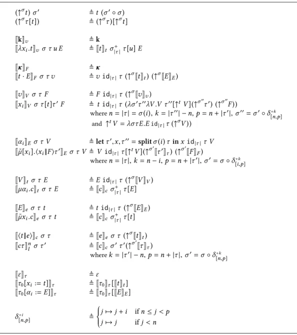
The translation of terms is given in Figure6, where we assume that for each constantk of typeX (resp. co-constantκ of type A⊥⊥) of the source system, we have a constant of typeX in the signatureS of target language, constant that we also denote byk (resp.κ of type A → ⊥). Except for the explicit renaming, the translation is the very same as in Ariolaet al., hence their results are preserved when considering a weak head-reduction strategy.

JkK σ v ≜ k Jλx .t K σ v τ u E ≜ Jt K σ [x:=n] t τ [n := u] E (n fresh) Jκ K σ F ≜ κ Jt·EK σ F τ v ≜ v τJt K σ t JE K σ E Jv K σ V τ F ≜ F τ Jv K σ v Jx K σ V τ [σ(x) := t]τ′F ≜ t τ (λτ λV .V τ [σ (x ) :=↑tV ]τ′F) (with ↑tV = λτE.E τ V ) Jα K σ E τ [σ(α ) := E]τ′V ≜ E τ [σ (α ) := E]τ′V Jµ[x].⟨x ||F ⟩τ˜ ′ K σ Eτ V ≜ V τ [n :=↑tV ]τ′′JF K σ′ F (where n fresh, τ′′,σ′=Jτ K σ [x:=n] τ ) JV K σ t τ E ≜ E τ JV K σ V Jµα .c K σ t τ E ≜ Jc K σ [α :=n] c τ [n := E] (n fresh) JE K σ e τ t ≜ t τ JE K σ E Jµx .c˜ K σ e τ t ≜ Jc K σ [x:=n] c τ [n := t] (n fresh) J⟨t ||e⟩K σ c τ ≜ Je K σ e τ Jt K σ t Jc τ K σ l τ0 ≜ _{Jc K}σ ′ c τ0τ ′ _{(where τ}′_,σ′₌ Jτ K σ τ) Jε K σ τ ≜ ε,σ Jτ ′_{[x := t]K}σ τ ≜ τ′[n := Jt K σ′ t ],σ[x := n] (where τ′,σ′= Jτ K σ τ, n fresh) Jτ ′_{[α := E]K}σ τ ≜ τ′[n := JE K σ′ E ],σ[α := n] (where τ′,σ′= Jτ K σ τ, n fresh)

Fig. 6. Translation of terms

Theorem 4.5. The translation is well-typed, i.e. 1. if Γ ⊢v v : A thenJΓ⊢vv : AK 2. if Γ ⊢F F : A⊥⊥thenJΓ⊢F F : A ⊥ ⊥ K 3. if Γ ⊢V V : A thenJΓ⊢V V : AK 4. if Γ ⊢EE : A⊥⊥thenJΓ⊢E E : A ⊥ ⊥ K 5. if Γ ⊢t t : A thenJΓ⊢t t : AK 6. if Γ ⊢e e : A⊥⊥thenJΓ⊢ee : A ⊥ ⊥ K 7. if Γ ⊢c c thenJΓ⊢ccK 8. if Γ ⊢l l thenJΓ⊢l lK 9. if Γ ⊢τ τ :Γ′thenJΓ⊢τ τ :Γ ′ K

Proof. The proof is an induction over the typing rules. As this induction is space-consuming

and mostly consists in a tedious verification that the typing derivation are indeed constructible for

the translated sequent, we give it in AppendixCtogether with the few technical lemmas that are

necessary. □

Combining the preservation of reduction through the CPS and a proof of normalization of our

target language (that one could obtain for instance using realizability techniques again), the former

theorem would provides us with an alternative proof of normalization of theλ_lv- andλ[lvτ ⋆]-calculi.

5 INTRODUCING DE BRUIJN INDEXES 5.1 The need for α -conversion

As for the proof of normalization, we observe in Figure6that the translation relies on names which implicitly suggests ability to performα -conversion at run-time. Let us take a closer look at an example to better understand this phenomenon.

Example 5.1 (Lack of α -conversion). Let us consider a typed closure ⟨t ||e⟩τ such that: πt Γ ⊢tt : A πe Γ ⊢e e : A⊥⊥ Γ ⊢c ⟨t ||e⟩ πτ ⊢_ττ :Γ ⊢_l ⟨t ||e⟩τ

Assume that botht and e introduce a new variable x in their sub-derivations π_tandπ_e, which will be the case for instance ift= µα.⟨u|| ˜µx.⟨x||α⟩⟩ and e = ˜µx.⟨x ||F⟩. This is perfectly suitable for typing, however, this command would reduce (withoutα -conversion) as follows:

⟨µα .⟨u || ˜µx .⟨x ||α ⟩⟩|| ˜µx .⟨x ||F ⟩⟩ → ⟨x ||F ⟩[x := µα.⟨u|| ˜µx.⟨x||α⟩⟩] → ⟨µα .⟨u || ˜µx .⟨x ||α ⟩⟩|| ˜µ[x].⟨x ||F ⟩⟩ → ⟨u || ˜µx .⟨x ||α ⟩⟩[α := ˜µ[x].⟨x||F⟩] → ⟨x ||α ⟩[α := ˜µ[x].⟨x ||F⟩,x := u] → ⟨x || ˜µ[x].⟨x ||F ⟩⟩[α := ˜µ[x].⟨x ||F⟩,x := u] → ⟨x ||F ⟩[α := ˜µ[x].⟨x||F⟩,x := u,x := x] → ⟨x || ˜µ[x].⟨x ||F ⟩⟩[α := ˜µ[x].⟨x||F⟩,x := u] →. . .

This command will then loop forever because of the auto-reference [x := x] in the store.

This problem is reproduced through a naive CPS translation without renaming (as it was originally

defined in [2]). In fact, the translation is somewhat even more problematic. Since "different" variables x (that is variables which are bound by different binders) are translated independently (e.g.J⟨t ||e⟩Kis defined from

Je KandJt K), there is no hope to performα -conversion on the fly during the translation. Moreover, our translation (as well as the original CPS in [2]) is defined modulo administrative

translation (observe for instance that the translation of Jλx .v K

σ

v τ V makes the λx binder vanish).

Thus, the problem becomes unsolvable after the translation, as illustrated in the following example.

Example 5.2 (Lack of α -conversion in the CPS). The naive translation (i.e. without renaming) of the same closure is again a program that will loop forever:

Jcε K = Je KeεJt Kt =Jµx .⟨x ||F ⟩˜ KeεJt Kt =J⟨x ||F ⟩Kc[x :=Jt Kt] =Jx Kx [x :=Jt Kt]JF KF =Jµα .⟨u || ˜µx .⟨x ||α ⟩⟩Ktε (λτλV .V τ [x :=↑ t V ]JF KF) =J⟨u || ˜µx .⟨x ||α ⟩⟩Kt [α := λτλV .V τ [x :=↑ t_{V ]} JF KF] =Jµx .⟨x ||α ⟩˜ Ke [α := λτλV .V τ [x :=↑ t_{V ]} JF KF]Ju Kt =J⟨x ||α ⟩Kc [α := λτλV .V τ [x :=↑ t V ]JF KF,x :=Ju Kt] =Jα KE [α := λτλV .V τ [x :=↑ t_{V ]} JF KF,x :=Ju Kt]Jx KV = (λτλV .V τ [x :=↑t_{V ]) [α := λτλV .V τ [x :=↑}t_{V ]} JF KF,x :=Ju Kt]Jx KV →_{Jx KV} [α := λτλV .V τ [x :=↑tV ] JF KF,x :=Ju Kt,x :=Jx Kt]

Observe that as the translation is defined modulo administrative reduction, the first equations

indeed are equalities, and that when the reduction is performed, the two "different"x are not bound anymore. Thus, there is no way to achieve any kind ofα -conversion to prevent the formation of the cyclic reference [x :=

Jx KV].

This is why we would need either to be able to performα -conversion while executing the translation of a command, assuming that we can find a smooth way to do it, or to explicitly handle

the renaming as we did in Section4. As highlighted by the next example, this problem does not occur with the translation we defined, since two different fresh names are attributed to the "different"

variablesx.

Example 5.3 (Explicit renaming). To compact the notations, we will write [x_m|_γα|...] for the renam-ing substitution [x := m,α := γ ,...], where we adopt the convention that the most recent binding is written on the right. As a binding [x := n] overwrites any former binding [x := m], we write [_γα|x_n] instead of [x_m|_γα|_nx]. Jcε K ε ₌ Je K ε eεJt K ε t =Jµx .⟨x ||F ⟩˜ K ε eεJt K ε t =J⟨x ||F ⟩K [x_m] c [m := Jt Kt] =Jx K [x_m] t [m := Jt K ε t] JF K [_mx] F =Jµα .⟨u || ˜µx .⟨x ||α ⟩⟩K [x_m] t ε(λτλV .V τ [m :=↑tV ]JF K [x_m] F ) =J⟨u || ˜µx .⟨x ||α ⟩⟩K [x_m|α_γ] t [γ := λτλV .V τ [m :=↑t V ] JF K [_mx] F ] =Jµx .⟨x ||α ⟩˜ K [x_m|_γα] e [γ := λτλV .V τ [m :=↑tV ] JF K [x_m] F ] Ju K [x_m|_γα] t =J⟨x ||α ⟩K [x:=m,α:=γ,x:=n] c [γ := λτλV .V τ [m :=↑tV ] JF K [x_m] F ,n :=Ju K [x_m|α_γ] t ] =Jα K [x_m|_γα|x_n] E [γ := λτλV .V τ [m :=↑t V ] JF K [_mx] F ,n :=Ju K [x_m|_γα] t ] Jx K [x_m|α_γ|x_n] V = (λτλV .V τ [m :=↑tV ]) [γ := λτλV .V τ [m :=↑tV ]JF K [_mx] F ,n :=Ju K [x_m|α_γ] t ] Jx K [_γα|_nx] V →_{Jx K}[ α γ|x_n] V [γ := λτλV .V τ [m :=↑tV ] JF K [x_m] F ,n :=Ju K [_mx|_γα] t ,m :=Jx K [α_γ|x_n] t ] =Jx K [α_γ|x_n] V [γ := λτλV .V τ [m :=↑tV ] JF K [x_m] F ,n :=Ju K [_mx|_γα] t ,m :=Jx K [α_γ|_nx] t ]

We observe that in the end, the variablem is bound to the variable n, which is now correct.

Another way of ensuring the correctness of our translation is to correct the problem already

in theλ[lvτ ⋆], using what we call De Bruijn levels [9]. As we observed in the first example of

this section, the issue arises when adding a binding [x := ...] in a store that already contained a variablex. We thus need to ensure the uniqueness of names within the store. An easy way to do this consists in changing the names of variable bound in the store by the position at which they

occur, which is obviously unique. Just as De Bruijn indexes are pointers to the correct binder, De

Bruijn levels are pointers to the correct cell of the environment. Before presenting formally the

corresponding system and the adapted translation, let us take a look at the same example that we

reduce using this idea. We use a mixed notation for names, writingx when a variable is bound by a λ or a ˜µ, and xi (wherei is the relevant information) when it refers to a position in the store.

Example 5.4 (Reduction with De-Bruijn levels). The same reduction is now safe if we replace stored variable by their De Bruijn level:

⟨µα .⟨u || ˜µx .⟨x ||α ⟩⟩|| ˜µx .⟨x ||F ⟩⟩ → ⟨x0||F ⟩[x0:= µα.⟨u|| ˜µx.⟨x||α⟩⟩] → ⟨µα .⟨u || ˜µx .⟨x ||α ⟩⟩|| ˜µ[x].⟨x ||F ⟩⟩ → ⟨u || ˜µx .⟨x ||α0⟩⟩[α0:= ˜µ[x].⟨x||F⟩] → ⟨x1||α0⟩[α0:= ˜µ[x].⟨x||F⟩,x1:= u] → ⟨x1|| ˜µ[x].⟨x ||F ⟩⟩[α0:= ˜µ[x].⟨x ||F⟩,x1:= u] → ⟨x2||F ⟩[α0:= ˜µ[x].⟨x||F⟩,x1:= u,x2:= x1] → ⟨x1|| ˜µ[x].⟨x ||F ⟩⟩[α0:= ˜µ[x].⟨x ||F⟩,x1:= u] → ⟨u ||F ⟩[α0:= ˜µ[x].⟨x||F⟩,x1:= u,x2:= u]

5.2 The λ[lvτ ⋆]-calculus with De Bruijn levels

We now use De Bruijn levels for variables (and co-variables) that are bound in the store. We use the

mixed notation9x_iwhere the relevant information isx when the variable is bound within a proof (that is by aλ or ˜µ binder), and where the relevant information is the number i once the variable has been bound in the store (at positioni). For binders of evaluation contexts, we similarly use De Bruijn levels, but with variables of the formα_i, where, again,α is a fixed name indicating that the variable is binding evaluation contexts, and the relevant information is the indexi.

The corresponding syntax is now given by:

Strong values v ::= k | λx_i.t Weak values V ::= v | x_i Terms t ,u ::= V | µα_i.c Forcing contexts F ::= κ | t · E Catchable contexts E ::= F | α_i | ˜µ[x_i].⟨x_i||F ⟩τ Evaluation contexts e ::= E | ˜µx_i.c Stores τ ::= ε | τ [x_i := t] | τ [α_i := E] Commands c ::= ⟨t ||e⟩ Closures l ::= cτ

As the store can be dynamically extended during the execution, the emplacement of a term in

the store and the corresponding pointer are likely to evolve (monotonically). Therefore, we need to

be able to update De Bruijn levels within terms (contexts, etc...). To this end, we define the lifted

term↑+_nit as the term t where all the free variables x_j withj > n (resp. α_j) have been replaced by x_j+i. Formally, they are defined as follows10:

↑+_ni(k) _{≜ k} ↑_n+i(λx_j.t ) _{≜ λ(↑n}+ixj).(↑+nit) ↑+_ni(x_j) _{≜ xj} (if j < n) ↑+_ni(x_j) _{≜ xj+i} (if j ≥ n) ↑_n+i(µα_j.c) ≜ µ(↑+_niαi).(↑+nic) 9

Observe that we could also use usual De Bruijn indexes for bound variables within the terms 10

(k : A) ∈ S Γ ⊢vk : A (k) Γ,xn :A ⊢_tt : B |Γ| = n Γ ⊢vλxn.t : A → B (→r) Γ(n) = (xn :A) Γ ⊢V xn :A (x ) Γ ⊢vv : A Γ ⊢Vv : A (↑V) (κ : A) ∈ S Γ ⊢F κ : A⊥⊥ (κ ) Γ ⊢tt : A Γ ⊢E E : B ⊥ ⊥ Γ ⊢F t · E :(A → B)⊥⊥ (→l) Γ(n) = (αn :A⊥⊥) Γ ⊢Eαn:A⊥⊥ (α ) Γ ⊢F F : A ⊥ ⊥ Γ ⊢E F : A⊥ (⊥ ↑ E₎ Γ ⊢VV : A Γ ⊢tV : A (↑ t₎ Γ,αn :A ⊥ ⊥_⊢ cc |Γ| = n Γ ⊢t µαn.c : A (µ) Γ ⊢E E : A⊥⊥ Γ ⊢eE : A⊥⊥ (↑ e₎ Γ,xn:A ⊢cc |Γ| = n Γ ⊢e µx˜ _n.c : A⊥⊥ ( ˜µ) Γ,xi :A,Γ′⊢_F F : A⊥⊥ Γ,x_i :A ⊢_ττ :Γ′ |Γ| = i Γ ⊢E µ[x˜ _i].⟨x_i||F ⟩τ : A⊥⊥ ( ˜µ[]) Γ ⊢τ ε : ε (ε ) Γ ⊢τ τ :Γ′ Γ, Γ′⊢tt : A |Γ, Γ′|= n Γ ⊢τ τ [xn := t] : Γ′,x_n :A (τt) Γ ⊢τ τ :Γ ′ _{Γ, Γ}′_⊢ E E : A⊥⊥ |Γ, Γ′|= n Γ ⊢τ τ [αn := E] : Γ′,α_n :A⊥⊥ (τE) Γ ⊢t t : A Γ ⊢ee : A⊥⊥ Γ ⊢c ⟨t ||e⟩ (c ) Γ, Γ′_⊢ cc Γ ⊢τ τ :Γ′ Γ ⊢lcτ (l )

Fig. 7. Typing rules for the λ[lvτ ⋆]-calculus with De Bruijn

The reduction rules become:

⟨t || ˜µxi.c⟩τ → c[xn/xi]τ [x_n := t] with|τ |= n ⟨µα .c ||E⟩τ → c[αn/αi]τ [α := E] with|τ |= n

⟨V ||αn⟩τ → ⟨V ||τ(n)⟩τ

⟨xn||F ⟩τ [xn := t]τ′ → ⟨t || ˜µ[x_n].⟨x_n||F ⟩τ′⟩τ

⟨V || ˜µ[xi].⟨x_i||F ⟩τ′⟩τ → ⟨V ||↑+_niF ⟩τ [x_n := V ](↑+_niτ′) with |τ | = n ⟨λxi.t ||u · E⟩τ → ⟨u || ˜µxn.⟨t[xn/xi]||E⟩⟩τ with|τ |= n

Note that we choose to perform indexes substitutions as soon as they come (maintaining the

property thatx_nis a variable referring to the(n + 1)thelement of the store), while it would also have been possible to store and compose them along the execution (so thatx_nis a variable referring to the(σ (n) + 1)thelement of the store whereσ is the current substitution). This could have seemed more natural for the reader familiar with compilation procedures that do not modify at run time

but rather maintain the location of variables through this kind of substitution.

The typing rules are unchanged except for the one where indexes should now match the length

of the typing context. The resulting type system is given in Figure7.

5.3 System Fϒwith De Bruijn levels

The translation for judgments and types are almost the same than in the previous section, except

that we avoid using names and rather use De Bruijn indexes. For instance, we define11:

JΓ⊢ee : A

⊥ ⊥

K ≜ ⊢ Je Ke :JΓKΓ▷eι(A) ϒ ▷eA ≜ ∀Y <: ϒ. Y → (Y ▷tA) → ⊥

The target language is again an adaptation of System F with stores (lists), in which store subtyping

is now witnessed by explicit coercions.

11