HAL Id: halshs-00763675
https://halshs.archives-ouvertes.fr/halshs-00763675v2
Preprint submitted on 26 Sep 2013
HAL is a multi-disciplinary open access
archive for the deposit and dissemination of sci-entific research documents, whether they are pub-lished or not. The documents may come from teaching and research institutions in France or
L’archive ouverte pluridisciplinaire HAL, est destinée au dépôt et à la diffusion de documents scientifiques de niveau recherche, publiés ou non, émanant des établissements d’enseignement et de recherche français ou étrangers, des laboratoires
farming in China: a case study of paddy rice production
Huanxiu Guo, Sébastien Marchand
To cite this version:
Huanxiu Guo, Sébastien Marchand. The environmental efficiency of non-certified organic farming in China: a case study of paddy rice production. 2013. �halshs-00763675v2�
The environmental efficiency of non-certified organic farming in China: a
case study of paddy rice production
Huanxiu Guo and S´ebastien Marchand
Etudes et Documents n◦38
Novembre 2012
CERDI
65 BD. F. MITTERRAND
63000 CLERMONT FERRAND - FRANCE TEL. 04 73 71 74 20
FAX 04 73 17 74 28
Les auteurs / The authors
Huanxiu Guo
Doctorant / PhD Student
Clermont Universit´e, Universit´e d’Auvergne, CNRS, UMR 6587, CERDI, F-63009 Clermont Fd, France.
Email : huanxiu.guo@etu-udamail.fr
Sebastien Marchand
Maitre de Conf´erence en ´economie
Clermont Universit´e, Universit´e d’Auvergne, CNRS, UMR 6587, CERDI, F-63009 Clermont Fd, France.
Email : sebastien.marchand@udamail.fr
La s´erie des Etudes et Documents du CERDI est consultable sur le site :
http://www.cerdi.org/ed
Directeur de la publication : Patrick Plane
Directeur de la r´edaction : Catherine Araujo Bonjean Responsable d’´edition : Annie Cohade
ISSN : 2114 7957
Avertissement :
Les commentaires et analyses d´evelopp´es n’engagent que leurs auteurs qui restent seuls responsables des erreurs et insuffisances.
R´esum´e / Abstract
This case study compares the environmental efficiency of non-certified organic and conventional rice production in southern China. Using plot–season level sur-vey data, we first test the existence of a “technology gap” between the two types of production, and then calculate the environmental efficiency scores based on the use of pure nitrogen, which is considered as an environmentally detrimen-tal input within the framework of the stochastic frontier analysis. Our analysis reveals that organic farming loses its environmental performance at high nitro-gen levels and especially during the initial expansion period of organic farming as newly converted organic farmers prefer to increase the use of external nutri-ents such as nitrogen to compensate for a potential yield loss. These results highlight the uncertainty with which conventional farmers tend to view organic farming. However, we find that the experience gained by organic farmers over time helps increase and maintain their environmental efficiency. We thus warn against the rapid expansion of organic farming and recommend more technical support and strict nutrient regulation to maintain the environmental efficiency of organic farming.
Mots cl´es / Key words : Organic farming, Environmental efficiency, Stochastic frontier analysis, China.
Codes JEL / JEL codes : Q12, Q57, R15, O53, D71
Remerciements / Acknowledgements
We thank the participants of the second conference on Environment and Resource Management in Developing and Transition Countries held at CERDI (University of Auvergne) in Clermont-Ferrand (October 2012), the participants of the 2013 INFER annual conference held at LEO (University of Orleans) in Orleans (may 2013), and Chlo´e Duvivier, Pascale Combes Motel, Mohamed Chaffai and Steven Helfand for their useful comments. We would like to thank the NGO Partnerships for Community
Devel-1
Introduction
Achieving the balance between yield and the preservation of the agro-environment has always been the biggest challenge in agricultural development. Within this context, the debates about the sustainability of conventional and organic farming have never ceased (Avery, 1998; Pretty and Hine, 2001; Badgley et al., 2007; Connor, 2008). This debate is now becoming a critical and urgent issue in the 21st century, as the ever-increasing world population requires higher agricultural yields whilst the deterioration of the agro-environment is becoming more and more serious due to modern agriculture’s excessive dependence on environmentally detrimental inputs.
Advocates of organic farming argue that organic farming is more environmentally friendly given its exclusion of synthetic inputs, i.e., pesticides, herbicides and fertilisers. Evidence shows that organic farming has significant environmental benefits in terms of agricultural pollution reduction, soil and water conservation, soil fertility recovery, eco-logical health and biodiversity improvement. This argument has been supported by world institutions who have promoted organic farming on a global scale (Willer et al.,2009;FAO,
2002; IFAD, 2002; WorldBank, 2009; Twarog,2006; Kilcher,2007;Hine et al., 2008). On the other side of the debate, critics of organic farming firstly stress the lower productivity of organic farming. Studies show that conversion to certified organic farming could reduce agricultural productivity by 20-50 percent in Europe and North America (Avery, 1998;
Connor, 2008;Mayen et al.,2010).
Moreover, an often neglected concern involves the pollution of organic nutrients. In-deed, excessive use of external nutrients from organic sources also has a negative environ-mental impact. For example, the leaching of organic nitrates can cause water pollution, and ammonia volatilization of animal manure is a main source of greenhouse gas from agriculture (Pretty, 1995; Kirchmann et al., 1998). Therefore, to evaluate agricultural sustainability, one must take account of both agricultural productivity and efficient use of external nutrients. While many studies have focused on the productivity of organic farming (Avery, 1998; Connor, 2008; Pretty and Hine, 2001; Badgley et al., 2007), little attention has been given to the study of nutrient use in organic farming, especially for
non-certified organic farming in developing countries1.
In the literature of efficiency study, Reinhard et al. (1999) propose an indicator of environmental efficiency (hereafter referred to as EE) which is defined as the ratio of minimum feasibility to the observed use of an environmentally detrimental input at given output level. In other words, the indicator of EE measures the efficient use of environmen-tally detrimental inputs in agriculture production. This measure is appropriate for the evaluation of organic farming systems and provides useful insights into its environmental performance compared to conventional farming systems. In this paper, we contribute to the literature by applying the environmental efficiency to evaluate smallholder paddy rice production in a Chinese village, where non-certified organic farming was introduced in the context of the New Rural Reconstruction movement (Renard and Guo,2013). Specifically, we focus on the efficient use of pure nitrogen, the most important nutrient input for paddy rice production. Meanwhile, it is also the biggest pollutant to air and underground water resulting from agricultural production in China (Zhu and Chen, 2002;Ju et al., 2007)2.
Using plot-season level survey data and agronomic experiment data, we gathered our-selves in the village, we firstly test the hypothesis of a “technology gap” between non-certified organic and conventional farming to determine the right specification of the pro-duction function. We then calculate environmental efficiency scores using a Stochastic Frontier Analysis (SFA) approach for both organic and conventional plots. Finally, we compare the calculated environmental efficiency scores between organic and conventional farming. The panel structure of data (five seasons from 2008 to 2010) also allows us to investigate the evolution of environmental efficiency over time.
Our case study demonstrates that for smallholder rice production, conversion to or-ganic farming does not reduce the actual rice yield if chemical fertilizers are successfully substituted with organic nutrients. There is no significant “technology gap” between or-1Organic farming systems and products are not always certified and are referred to as “non-certified
organic farming or products”. Non-certified organic farming systems are prevalent in developing countries although it is difficult to quantify to what extent.
2Environmental efficiency can be derived from different models such as the one ofCuesta et al.(2009)
in which environmental damage is analysed through “bad output” modelling. In our case study, this strategy cannot be implemented because we have no information regarding the environmental damage caused by rice farming. For instance, we have no information on water or air pollution. For this reason, we focus only on the efficient use of an environmentally detrimental input, i.e., pure nitrogen.
ganic and conventional farming in poor areas. However, organic farming is not necessarily more environmentally efficient than conventional farming at high nutrient levels, which is mainly due to the inexperience of newly converted farmers in organic farming, especially during the initial conversion period from conventional to organic farming. Therefore, to maintain the environmental efficiency of organic farming, more external support such as technical training and environmental education are needed to accompany farmers during the conversion period.
The remainder of this paper is organized as follows. Section 2 presents the organic farming project in the village. Section 3 describes the methodological framework and empirical method. Section 4 gives details of the data. Section 5 discusses the main results and Section 6 concludes.
2
Organic farming in Sancha village
Originally dedicated to produce high quality products for exportation, organic farming has now become a rural development strategy in China. Since 2003, vibrant organic communities have been observed in rural China in conjunction with the social movement of the New Rural Reconstruction that was initiated by scholars, students and social activists. Diverse models such as farmer’s co-ops, farmer-participatory development and Community Supported Agriculture (CSA) have recently emerged to promote organic farming in China (Day, 2008; Jia’en and Jie, 2011). In this study, we will focus on one of these alternative models in southern China.
The study area is located in Sancha village (109.01E/22.73N), a small village in Hengzhou county of Guangxi province (see Map A in the Appendix)3. Due to the abun-dant water resources and tropical climate, paddy rice is one of the most important crops in this region. Since the 1960’s, machinery and modern chemical inputs have been pro-moted in southern China. However, given its remote situation and poverty, Sancha village maintains its old tradition of paddy rice production, e.g., two crop seasons of rain fed 3Guangxi Zhuang autonomous region is a minority “Zhuang” dominated region where the economic
culture, cattle tillage and the use of cow dung fertilizer. The average chemical fertilizer application level is about 16.76 kg per mu (1 mu = 1/15 ha) in the village, which is much lower than the average provincial level of 26.24 kg per mu4. Therefore, both the traditional agricultural practice and the well preserved natural environment favor the development of organic farming in this village.
In 2005, an organic farming project was introduced to the village by the local Maize Research Institution in partnership with an NGO called Partnerships for Community Development (PCD), with the aim of promoting organic paddy rice production5. This
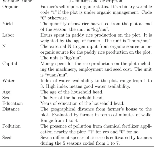
project began with participatory experimentation among a small group of farmers. During the experimentation period, the PCD provided strong technical and marketing support (CSA) to encourage conversion. By means of these participatory farmer experimentations, organic farmers found a suitable nutrient formula to substitute the chemical fertilizer by self–produced compost and traditional organic inputs6. With respect to pest control, farmers have adopted the integrated rice–duck culture system and the use of traditional medicinal plants, which appear to be efficient in preventing certain pests7. Table 1 gives more details about the difference between organic farming and conventional farming in Sancha village.
Table 1: Organic farming versus conventional farming in Sancha village
4Data comes from our household survey at the village-level and from the 2010 Guangxi Statistical
Year Book at the provincial level.
5PCD is based in Hong Kong. More information about this NGO can be found from their site:
http://www.pcd.org.hk/eng/index.html.
6Compost is produced by farmers using fish powder, bone powder, tea bran, peanut bran and bio gas
slurry.
7The integrated rice–duck system consists of organic rice culture and, in the mean time, raising ducks
Organic Conventional
Seeds Hybrid rice CY998,
Tradi-tional rice varieties: BX139, GF6, GF2, BGX, SYZ
Hybrid rice CY998
Fertilizers Compost(30% fish powder,
30% bone powder, 30%
peanut bran, 10% straw ash), Cow dung, Hen manure, Pig
manure, Bio gas slurry, Green manure
Cow dung, Pig manure, Green manure, Compound fertilizer,
Pest control Duck, Chinese medical plant Triazophos, Avermectins
Weed control Duck, Hand weeding Pretilachlor
Source: local agronomist of PCD
As one can note from table 1, the organic farming is more environmentally sound comparing to conventional farming. The use of chemical fertilizers and pesticides are strictly prohibited. Farmers adopt their own formula of fertilizers (i.e., compost, cow dung, pig manure, hen manure etc.) and seeds according to the availability and specific soil condition. More ecological methods such as duck raising have been integrated into the paddy rice production, which is expected to achieve the recurrence of ecosystem. Although without official organic certification, Sancha’s organic farming corresponds to the definition of non-certified organic farming according to the International Federation of Organic Agriculture Movements (IFOAM).
After three years of experimentation, the project entered into a novel phase of scaling up. The year of 2009 was a critical time point of the project. Thanks to the improved social networks, more farmers got access to information about the organic farming project8. An
acceleration of conversion to organic farming was observed in 2009. At the end of 2009, 73 percent of farmers in the village had conducted experiments on their paddy land. However, due to the limited resource of PCD, the technical support and environmental education was not able to cope with such a rapid expansion of organic farming. We note that although organic farming was universally accepted primarily due to its high price premium, newly converted farmers were still concerned about the loss of yield due to conversion.
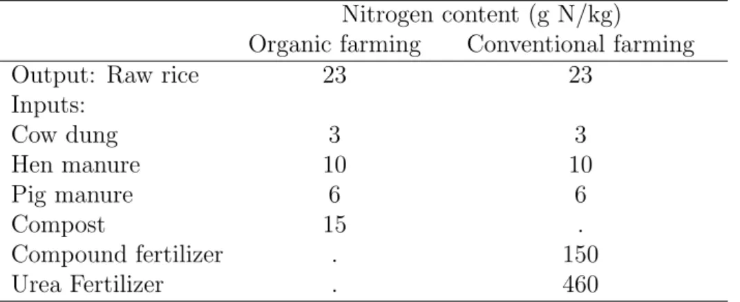
To investigate the performances of organic and conventional farming in Sancha village, we collected data on inputs and output of paddy rice production by means of a household survey. Combined with the agronomic experimentation data of nitrogen content for each input provided by the local agronomist (see Table 11 in the Appendix for more details), we were able to calculate the pure nitrogen input as well as the soil surface nitrogen balance for both systems9. Table 2 presents a comparative summary of agricultural and
envi-8More details about the social network construction in the village can be found in (Renard and Guo,
2013).
ronmental performance between conventional and organic farming during five consecutive crop seasons (from 2008 to 2010).
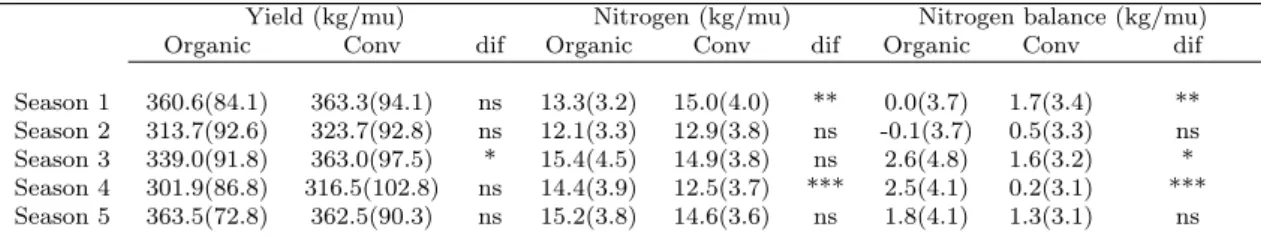
Table 2: Performance of organic and conventional farming in Sancha village
Yield (kg/mu) Nitrogen (kg/mu) Nitrogen balance (kg/mu) Organic Conv dif Organic Conv dif Organic Conv dif Season 1 360.6(84.1) 363.3(94.1) ns 13.3(3.2) 15.0(4.0) ** 0.0(3.7) 1.7(3.4) ** Season 2 313.7(92.6) 323.7(92.8) ns 12.1(3.3) 12.9(3.8) ns -0.1(3.7) 0.5(3.3) ns Season 3 339.0(91.8) 363.0(97.5) * 15.4(4.5) 14.9(3.8) ns 2.6(4.8) 1.6(3.2) * Season 4 301.9(86.8) 316.5(102.8) ns 14.4(3.9) 12.5(3.7) *** 2.5(4.1) 0.2(3.1) *** Season 5 363.5(72.8) 362.5(90.3) ns 15.2(3.8) 14.6(3.6) ns 1.8(4.1) 1.3(3.1) ns Notes: Data from the author’s household survey and agronomic experimentation data provided by the local agronomist. 1 mu = 1/15 ha. The mean value is presented with standard deviation in parentheses. Seasons 1–2, 3–4 and 5 cover 2008, 2009 and 2010 separately. *** statistical significance at 0.1%, ** statistical significance at 1%, * statistical significance at 5%. “ns” means non–significant.
From Table 2, we note that organic farming has successfully coped with conventional farming in terms of yield. There has been no significant difference between organic farming and conventional farming in five crop seasons. This is in line with similar observations from other developing countries (Zhu et al., 2000; Pretty et al., 2003) and can probably be explained by the similar pure nitrogen input in the village. As one can note, during the scale-up period (since season three in 2009), organic farmers tended to use more pure nitrogen than their non-organic counterparts. This is indeed not surprising and has already been highlighted in the literature. For instance,Hessel Tjell et al.(1999) andTorstensson
(2003) have reported that mean use of nitrogen in organic systems is close to that of conventional systems in Sweden. This phenomenon could be explained by the smallholder production on tiny plots, where it is quite possible to substitute chemical nitrogen with organic nitrogen. However, it is also certainly due to the behavior of newly converted farmers to organic farming in Sancha village. According to the head of the farmers’ association: “Since they (newly converted farmers) have less experience and confidence, they would generally apply more compost or animal manure for fear of yield loss from conversion.”
as the difference between the total quantity of pure nitrogen entering and the quantity of pure nitrogen leaving the soil surface over one production cycle. Since the aim of this approach is to investigate the global environmental impact of rice production, we do not distinguish between the loss of nitrogen to ground water and air separately.
Regarding the environmental impact, we take a look at the soil surface nitrogen bal-ance. A persistent deficit in nutrient budgets might indicate mining of soil nutrients, whilst a persistent surplus might indicate potential environmental pollution (OECD, 2001). We note that, at the mean level, both organic and conventional farming have displayed a varying nitrogen surplus, ranging from -0.1 kg per mu to 2.6 kg per mu. Compared to other Chinese provinces, the nitrogen surplus level in Sancha village is still low (Sun and Bouwman,2008;Wang et al.,2007) while compared to its neighbor countries such as Thai-land, Bangladesh and Vietnam, it appears to be at a similar or higher level (Wijnhoud et al.,2003;Hossain et al.,2012;Mussgnug et al.,2006). Once again, the nitrogen balance indicates a significant loss of environmental performance for organic farming during the scale–up period, which highlights the necessity of nitrogen optimization.
To summarize, in five consecutive crops seasons, organic farmers in Sancha village have achieved a satisfactory yield by substituting the chemical fertilizers with self–produced organic fertilizers. This is a big success from an economic point of view. However, the environmental cost is still high as indicated by high pure nitrogen input and nitrogen ac-cumulation in the soil, especially during the scale-up period. Therefore, in order to inves-tigate the sustainability of organic farming, we will need another indicator of nitrogen-use efficiency which takes into account both yield and environmental cost. For this purpose, we now turn to the indicator of environmental efficiency (EE) using the stochastic frontier analysis (SFA).
3
Methodological framework
The term of environmental efficiency used in this study is defined by the minimum use of pure nitrogen for a given level of yield. This environmental efficiency is different from conventional technical efficiency (TE) and stresses the efficient use of pure nitrogen, and thus the efficiency of environment preservation. Environmental efficiency is calculated from technical efficiency with the classic approach of SFA. We apply a two–step approach here as proposed by Reinhard et al. (1999). Environmental efficiency is firstly calculated from technical efficiency using a stochastic frontier analysis and then used as a dependent
variable to investigate the environmental efficiency of organic farming.
3.1
Calculating environmental efficiency with a SFA model
To determine the environmental efficiency of organic farming, we need first to calculate this efficiency. The way to achieve this is to introduce environmental variables into a tra-ditional production function in order to derive environmental efficiency from adjustments of conventional measures of technical efficiency.
Technical efficiency is first derived from a production frontier under the hypothesis that a non–optimal use of production factors by agricultural farmers, i.e., an X–inefficiency (Leibenstein,1966), is the effect of labor and credit constraints. Assuming that a farmer i uses traditional X inputs to produce single or multiple conventional Y outputs, a pro-duction function can be written to represent a particular technology: Yi = f (xi), where
f (xi) is a production frontier. On the frontier, the farmer produces the maximum output
for a given set of traditional inputs or uses the minimum set of traditional inputs to pro-duce a given level of output. In standard microeconomic theory, there is no inefficiency in the economy, implying that all production functions are optimal and all firms produce at the frontier. However, if markets are imperfect, farmers’ yields can be pulled below the production frontier.
Consider now the environmental pollution of the agricultural production. Conven-tionally, environmental damage can be modeled as undesirable outputs (Cuesta et al.,
2009). However in our case, we cannot apply this method since we have no precise data regarding environmental damage such as water or air pollution related to agricultural pro-duction. Alternatively, we focus only on nitrogen as a source of environmental pollution. This environmentally detrimental input can be introduced in the function production. To be efficient, a farmer needs to maximize his conventional yield with the environmentally detrimental input, i.e. nitrogen, as well as with other conventional inputs (X).
In this context, we follow Reinhard et al. (1999) by defining environmental efficiency as the ratio of minimum feasibility to the observed use of the environmentally detrimental
input, conditional to observed levels of output and conventional inputs10. This can be formulated by the following non–radial input–oriented measure:
EEi(x, y) = [min θ : F (xi, θZi) ≥ yi], (1)
where the variable yi is the observed output for farmer i, produced using Xi of the
conventional inputs and Zi of the environmentally detrimental input. F (.) is the best
practise frontier with X and Z.
Within the framework developed by Reinhard et al. (1999), environmental efficiency can be calculated using a standard translog production function as follows (Christensen et al., 1971)11: ln(Yi,t) = β0+ m X j=1 βjln(Xij,t) + βzln(Zi,t) + 1 2 m X j=1 m X k=1 βjkln(Xji,t)ln(Xki,t) + 1 2 m X j=1 βjzln(Xji,t)ln(Zi,t) + 1 2βzzln(Zi,t) 2− U i,t+ Vi,t, (2)
where i = 1, . . . , n is the plot unit observations and t = 1, . . . , T is the number of periods; j, k = 1, 2, . . . , m is the applied traditional inputs; ln(Yi,t) is the logarithm of the output
of plot i; ln(Xij,t) is the logarithm of the jth traditional input applied on the ith plot;
ln(Zi,t) is the logarithm of the environmental detrimental input applied; and βj, βz, βjk,
βjz and βzz are parameters to be estimated12. The logarithm of the output of a technically
efficient producer YF
i,t with Xi,t and Zi,t can be obtained by setting Ui,t = 0 in Equation
2. However, the logarithm of the output of an environmentally efficient producer Yi,t with
Xi,t and Zi,t is obtained by replacing Zi,t by Zi,tF, where Zi,tF = EEi,t ∗ Zi,t, and setting
Ui,t = 0 in Equation 2 as follows
10Environmental efficiency is thus an input–oriented measure, i.e., less environmental detrimental input
with the same output and conventional inputs.
11We use a negative sign in order to show that the term −U
i,t represents the difference between the
most efficient farm (on the frontier) and the observed farm.
12Similarity conditions are imposed, i.e., β
jk= βkj. Moreover, the production frontier requires
mono-tonicity (first derivatives, i.e., elasticities between 0 and 1 with respect to all inputs) and concavity (negative second derivatives). These assumptions should be checked a posteriori by using the estimated parameters for each data point.
ln(Yi,t) = β0+ m X j=1 βjln(Xij,t) + βzln(Zi,tF) + 1 2 m X j=1 m X k=1 βjkln(Xji,t)ln(Xki,t) + 1 2 m X j=1 βjzln(Xji,t)ln(Zi,tF) + 1 2βzzln(Z F i,t) 2 + Vi,t. (3)
The logarithm of EE (lnEEi,t = lnZi,tF − lnZi,t) can now be calculated by setting
Equations 2 and 3 equal as follows:
1 2βzz(lnEEi,t) 2+ (lnEE i,t)[βz+ m X j=1
βjzlnXij,t+ βzzlnZi,t] + Ui,t. = 0 (4)
By solving Equation4, we obtain:
lnEEi,t = − A z }| { βz+ m X j=1 βjzlnXij,t+ βzzlnZi,t ± B z }| { βz+ m X j=1 βjzlnXij,t+ βzzlnZi,t − 2βzzUi,t 0.5 /βzz (5)
As mentioned by Reinhard et al. (1999), the output-oriented efficiency is estimated econometrically whereas environmental efficiency (Eq. 4) is calculated from parameter estimates (βz and βzz) and the estimated error component (Ui,t).
Since a technically efficient farm (Ui,t = 0) is necessarily environmentally efficient
(lnEEi,t = 0). The “ +
√00
must be used13.
In our case of paddy rice production, three traditional inputs and one environment detrimental input are identified for the production function. The final stochastic model
13The sign in front of term B should necessarily be positive. Thus, if U
in the translog case is as follows:
Y ieldi,t= β0+ β1.Li,t+ β2.Ci,t+ β3.Wi,t+ β4.Ni,t+ β5.Li,t2 + β6.Ci,t2 + β7.Wi,t2 + β8.Ni,t2 + β9.Li,t
∗ Ci,t+ β10.Li,t∗ Ni,t+ β11.Li,t∗ Wi,t+ β12.Ci,t∗ Wi,t+ β13.Ci,t∗ Ni,t+ β14.Ni,t∗ β15.Wi,t+ Seed
+ Season − Ui,t+ Vi,t.
(6)
Here the output is the yield of raw rice. The three traditional inputs are the labor (L), capital (C) and water (W ), and the environment detrimental input is the pure nitrogen input (N ) derived from both organic and chemical sources. All output and inputs are normalized by the plot area. Traditionally, farmers use different seeds in different seasons according to climate, we need to control for this in the equation with Season as a dummy fixing one of the five seasons and Seed as a dummy for different seed species (see Tables 3 and 12 for descriptive statistics, and Table 10 for description and definition of vari-ables). The inefficiency term is allowed to be time–variant following the Battese–Coelli parametrization of time-effects (Battese and Coelli,1992). Therefore, the maximum like-lihood estimator is appropriate to estimate technical efficiency, which is modeled as a truncated-normal random variable multiplied by a specific function of time14.
One fundamental question underlying the standard model above is whether organic and conventional farming share similar production technology. In other words, should we model these two types of production processes with a single production function? Con-ventionally, one may expect that the organic standards and chemical input constraints will significantly change the production process. If this is the case, a single production function modelling may yield biased technical efficiency, and thus biased environmental efficiency. It is therefore necessary to control for technology heterogeneity in the produc-tion funcproduc-tion or apply the meta–frontiers analysis (Battese and Rao, 2002;Battese et al.,
2004; Oˆa ˘A´ZDonnell et al., 2008).
However, we also have good reason to believe that the technology of organic and conventional farming may be similar in small and undeveloped rural areas, since poor farmers face a similar environment and cannot easily improve their production means
by simply switching to organic farming during such a short time. The major difference between organic and conventional farming is reflected by the amount of inputs which is modelled by the translog production function. In other words, organic farming would not directly but rather indirectly influence the productivity through the efficiency terms (i.e., TE and EE). If this is the case, a two-stage analysis is appropriate (Battese and Coelli,
1995). Therefore, to ensure the relevance of technical efficiency from the beginning, we will need to perform a preliminary statistical test to determine the right specification of our production function as follows:
Y ieldi,t = β0+ β1.Li,t+ β2.Ci,t+ β3.Wi,t+ β4.Ni,t+ β5.L2i,t+ β6.Ci,t2 + β7.Wi,t2 + β8.Ni,t2
+ β9.Li,t∗ Ci,t+ β10.Li,t∗ Ni,t+ β11.Li,t∗ Wi,t+ β12.Ci,t∗ Wi,t+ β13.Ci,t∗ Ni,t+ β14.Ni,t
∗ Wi,t+ β15.Organici,t+ Season + Seed − Ui,t+ Vi,t
(7)
In equation 7, a dummy Organic, stating if the plot is under organic farming, is ap-pended in the standard production function to capture any potential “technology gap” be-tween two technologies. Moreover, one may suspect that organic farming will also change the marginal contribution to output of each input. We thus append organic interactive terms with all inputs as in the following equation 8:
Y ieldi,t = β0+ β1.Li,t+ β2.Ci,t+ β3.Wi,t+ β4.Ni,t+ β5.L2i,t+ β6.Ci,t2 + β7.Wi,t2 + β8.Ni,t2
+ β9.Li,t∗ Ci,t+ β10.Li,t∗ Ni,t+ β11.Li,t∗ Wi,t+ β12.Ci,t∗ Wi,t+ β13.Ci,t∗ Ni,t+ β14.Ni,t
∗ Wi,t+ β15.Organici,t+ β16.Organici,t∗ Li,t+ β17.Organici,t∗ Ci,t+ β18.Organici,t∗
Wi,t+ β19.Organici,t∗ Ni,t+ Season + Seed − Ui,t+ Vi,t
(8)
The hypothesis of the existence of a “technology gap” will be verified by checking the joint significance of coefficients between the organic intercept and slope shifters (i.e., β15–β19).
ap-proach. In our case, the adoption of organic farming and agricultural output could be conjointly determined by some omitted environmental and personal factors (e.g., soil qual-ity and farmer abilqual-ity). These omitted variables may bias the coefficients as well as the significance of the variables associated to organic farming (additive and interaction terms). To deal with this issue, we run a within estimation which eliminates the bias due to all time-invariant factors. To get rid of any potential time-variant factors, we will perform a within-2SLS estimation and compare the results with that of the within estimation.
In our dataset, we have two available instruments which are (1) the presence of chem-ical fertilizer pollution near the plot (Pollution) and (2) the geographchem-ical distance from farmer’s house to the plot (Distance). On one hand, the presence of chemical fertilizer pollution near the plot will render organic farming non credible and thus discourage this practice. On the other hand, organic farming requires much more labor due to transport and application of organic compost and manure so that long distance from house to plot will thus discourage organic farming15. The validity of these instruments is tested by the
Sargan over-identification test whereas their power is analysed by both the Shea partial R2 and the F statistics of excluded instruments. According to the result of these tests, we determine the correct specification of the production function. We can then derive technical efficiency and calculate environmental efficiency using the Formula 5.
3.2
Estimating the effect of organic farming on environmental
efficiency
The second step of the analysis consists of comparing organic farming and conventional farming in terms of environmental efficiency, which is calculated from the first stage. To this end, we regress a simple econometric model as follows:
EEi,t= γ0+ γ1Organici,t+ γ2Agei,t+ γ3Sexi,t+ γ4Educi,t+ εi,t. (9)
15Note that in a small village like Sancha, few machines are used for the transport and application of
Equation 9 represents the relationship between environmental efficiency and organic farming. The coefficient γ1 before the dummy variable Organic captures the difference
of environmental efficiency between organic and conventional farming. Since environmen-tal efficiency is a measurement of managerial performance which could depend on farmer characteristics, we control for major observable characteristics such as age, sex and edu-cation level of the plot owner in the model. Once again, to deal with the endogeneity of organic farming, a within estimator is used to control for unobserved and time–invariant individual effects. For time-variant effects, we make use of the two instruments used in the first stage to test the similarity of the production technology between organic and conventional farming. As such, the presence of a neighbor’s chemical fertilizer pollution and the geographical distance from the plot are used and combined with the fixed effect to perform a Within-2SLS estimation.
According to agronomic experimentation in field, the productivity of organic farming is heterogenous on various levels of nitrogen application. This observation is supported by another study stating that the yield of organic farming is less sensitive to nitrogen over certain critical levels (Kirchmann and Ryan, 2004). Should this be the case for environmental efficiency?
We explore the heterogeneity in environmental efficiency scores of organic farming on different nitrogen levels to derive more precise understanding. Given the potential endogeneity of nitrogen input, we could not introduce this variable and its interaction term (crossed with organic) into the model directly. Alternatively, we split the total sample into three equal sub–samples according to three critical levels of nitrogen application: (1) a high sub–sample which contains one third of the observations under which the level of nitrogen is the highest (ln N > 3.42); (2) a low sub–sample of one third of the observations under which the level of nitrogen is the lowest (ln N < 3.20); (3) a medium sub–sample of one third of the observations between the two levels (ln N between 3.20 and 3.42). Equation 9 is then estimated with respect to each of the three sub–samples. We note that this alternative solution is not perfect given that we can only observe a heterogenous correlation between environmental efficiency and organic farming rather than a causal
effect.
Moreover, the effect of organic farming on environmental efficiency can be due to the level of training received by organic farmers. As mentioned in Section 2, newly converted farmers in Sancha village tend to use more nitrogen due to their uncertainty and lack of training. Newly converted farmers can thus experience very low environmental efficiency because they are less trained and have little experience about organic farming. With our dataset, we can test if trained farmers, i.e., those who participated in the early organic farming experimentation in 2005, are more environmentally efficient than newly converted farmers. With the name list provided by the NGO, we are able to identify households who have participated in the experimentation and converted to organic farming since then. We thus redo the estimation of equation 9 with the sample of trained farmers.
We can also test the explanation and the robustness of the heterogenous effect of organic farming on environmental efficiency according to nitrogen use by focusing on time. As mentioned in Section 2, the development of the organic project in Sancha village allows us to explore the variation of environmental efficiency over time. Promoted by the PCD, the organic project in the village has scaled up since 2009. Along with this scaling up, a boost of nitrogen use has been observed in organic farming. Intuitively, if the heterogenous effect exists, the environmental efficiency of organic farming may also be different before and after 2009. To this effect, we estimate the following equation:
EEi,t = α0+ α1Organici,t+ α22009i,t+ α32009 ∗ Organici,t+ α4Agei,t+ α5Sexi,t
+ α6Educi,t+ εi,t,
(10)
where the variable 2009 is a dummy of 1 if the season is in 2009 or after, and 0 otherwise (before 2009). The variable 2009 ∗ Organic is an interaction term which captures the difference of organic effects before and after 2009. We control for farmer’s age, sex and education level as in Equation 9. For the estimation of the model, the within and within-2SLS estimators are applied to correct for the endogeneity of organic farming and obtain consistent estimates.
4
Data and descriptive statistics
The data used for this study derived from a detailed survey conducted in Sancha village by one of the authors. For the purpose of comparative study, two plots (one organic and one conventional) were randomly selected for every active farmer from their reported paddy fields, and information about the rice production was then collected on the basis of the plot16. To ensure the reliability of organic practices reported by farmers, we also checked the answers against the records of the farmers’ association. Inconsistent answers were dropped from the dataset. Information was collected for the past five consecutive crops seasons (from 2008 to first half of 2010) with respect to output and inputs used on the plot.
The output consists of raw rice yield reported by farmers and expressed as kg per mu. Labor, capital and water are identified as three major conventional inputs, and the pure nitrogen is considered as the unique environmentally detrimental input for paddy rice production. For labor use, we asked farmers for labor time spent on each segment of a given rice production cycle such as soil plowing, plant setting, composting, fertilizer application, weed and pest control and harvesting. The final labor use is the sum of all segments and measured as hours per mu. The measure of capital refers to financial expenditures on machine use during the entire production cycle and is measured as yuan per mu. A measure of water use is introduced in the production function given that water is necessary for paddy rice production. However, this is also quite difficult to quantify. Given the lack of irrigation infrastructure, water consumption is expected to be constrained by water availability to the plot. We hereby construct a proxy variable, namely the index of water availability, which relies on average rain fall and mouse activity on the plot observed by farmers.
The calculation of pure nitrogen is derived from the experimentation data of nitrogen content provided by local agronomists and farmers’ self–reporting of nutrient inputs (e.g., quantity of chemical fertilizers, animal manure and compost, etc.). The calculation is the same as presented in Section 2 and expressed as kg per mu.
For other explanatory variables, socio–economic characteristics of households were collected. These characteristics include the age, sex and education level of the head of household. We also collected information on plot characteristics such as area, geograph-ical distance and nearby presence of fertilizer pollution spots. Table 3 gives descriptive statistics of the database and a summary of variable definitions can be found in Table 10 in the Appendix.
Table 3: Descriptive statistics by type of farming
Total(1,012) Organic Plot(345) Conv Plot(667) Equality test Mean Sd Mean Sd Mean Sd P-value Yield (kg/mu) 342.16 (94.46) 336.49 (88.15) 345.09 (97.5) 0.17 Labor (h/mu) 129.81 (54.01) 156.33 (55.29) 116.09 (47.92) 0 N (kg/mu) 14.13 (3.96) 14.42 (4.03) 13.97 (3.93) 0.08 Capital (yuan/mu) 74.17 (52.21) 76.53 (51.31) 72.95 (52.67) 0.3 Water (1-3) 2.51 (0.65) 2.56 (0.67) 2.49 (0.64) 0.14 Age 54.59 (12.59) 53.42 (12.47) 55.19 (12.62) 0.03 Sex 0.61 (0.49) 0.68 (0.47) 0.57 (0.5) 0 Education 3.64 (3.3) 3.79 (3.51) 3.56 (3.19) 0.29 Distance (1-4) 1.91 (0.87) 1.57 (0.65) 2.09 (0.91) 0 Pollution (1/0) 0.74 (0.44) 0.34 (0.48) 0.95 (0.22) 0
Note: For all tests of means, the null hypothesis is that the means are equal against a two–sided alternative. The confidence level is at 5%.
From the descriptive statistics, we note that organic farming is more labor intensive than conventional farming, which is explained by the additional work of compost fabri-cation and transportation, as well as farm management. This abundant and hard work seems to discourage male and more aged farmers to produce organic farming in the vil-lage. Finally, the influence of geographical distance and neighbor fertilizer pollution is significant for the choice of organic farming. In the following section, we will present the estimated results and the calculated environmental efficiency from the SFA as well as the estimated results regarding the effect of organic farming on environmental efficiency.
5
Results and discussion
5.1
Technology gap and specification of SFA model
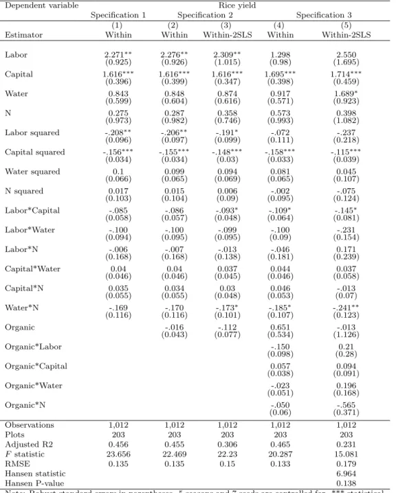
The first step is to test the hypothesis of “technology gap” between organic and conven-tional farming to determine the best specification of the SFA model. Three specifications (i.e., without controlling for organic farming, with organic additive intercept, and with organic additive intercept and interaction terms with each input) are thus estimated by the within and within-2SLS estimators (see Table 13 in the Appendix for the estimated results of the instrumentation equation). A comparison of estimated results are presented in Table 4.
In column 1 of Table 4, we estimate the standard SFA model and report it as a benchmark. One can note, in columns 2 and 3, that the inclusion of the organic variable in the model does not change many of the coefficients, and the organic intercept is also not significant. When the organic interaction terms are included in the model, the labor loses its significance. This is probably due to its correlation with the interaction term of Organic ∗ Labor. To check the hypothesis of a “technology gap”, we test the restrictions that the organic dummy and interaction terms are jointly equal to zero. The chi-squared statistic from a Wald test is 5.09 with an associated p-value of 0.405. Thus we cannot reject the null hypothesis that the organic intercept and slope shifters are jointly equal to 0 at conventional significance level. Put another way, the “technology gap” between organic and conventional farming is not significant in our case.
Table 4: Specification of SFA model
Dependent variable Rice yield
Specification 1 Specification 2 Specification 3 (1) (2) (3) (4) (5) Estimator Within Within Within-2SLS Within Within-2SLS Labor 2.271∗∗ 2.276∗∗ 2.309∗∗ 1.298 2.550 (0.925) (0.926) (1.015) (0.98) (1.695) Capital 1.616∗∗∗ 1.616∗∗∗ 1.616∗∗∗ 1.695∗∗∗ 1.714∗∗∗ (0.396) (0.399) (0.347) (0.398) (0.459) Water 0.843 0.848 0.874 0.917 1.689∗ (0.599) (0.604) (0.616) (0.571) (0.923) N 0.275 0.287 0.358 0.573 0.398 (0.973) (0.982) (0.746) (0.993) (1.082) Labor squared -.208∗∗ -.206∗∗ -.191∗ -.072 -.237 (0.096) (0.097) (0.099) (0.111) (0.218) Capital squared -.156∗∗∗ -.155∗∗∗ -.148∗∗∗ -.158∗∗∗ -.115∗∗∗ (0.034) (0.034) (0.03) (0.033) (0.039) Water squared 0.1 0.099 0.094 0.081 0.045 (0.066) (0.065) (0.069) (0.065) (0.107) N squared 0.017 0.015 0.006 -.002 -.075 (0.103) (0.104) (0.09) (0.095) (0.124) Labor*Capital -.085 -.086 -.093∗ -.109∗ -.145∗ (0.058) (0.057) (0.048) (0.064) (0.081) Labor*Water -.100 -.100 -.099 -.100 -.231 (0.094) (0.095) (0.095) (0.09) (0.154) Labor*N -.006 -.007 -.013 -.046 0.171 (0.168) (0.168) (0.138) (0.181) (0.239) Capital*Water 0.04 0.04 0.037 0.044 0.037 (0.046) (0.046) (0.045) (0.046) (0.058) Capital*N 0.035 0.034 0.03 0.046 -.013 (0.055) (0.055) (0.048) (0.053) (0.07) Water*N -.169 -.170 -.173∗ -.185∗ -.241∗∗ (0.116) (0.116) (0.101) (0.107) (0.123) Organic -.016 -.112 0.651 -.013 (0.043) (0.077) (0.534) (1.126) Organic*Labor -.150 0.21 (0.098) (0.28) Organic*Capital 0.057 0.094 (0.038) (0.091) Organic*Water -.023 0.196 (0.051) (0.168) Organic*N -.050 -.565 (0.06) (0.371) Observations 1,012 1,012 1,012 1,012 1,012 Plots 203 203 203 203 203 Adjusted R2 0.456 0.455 0.306 0.465 0.231 F statistic 23.656 22.469 22.23 20.287 15.081 RMSE 0.135 0.135 0.15 0.133 0.179 Hansen statistic 6.964 Hansen P-value 0.138
Note: Robust standard errors in parentheses. 5 seasons and 7 seeds are controlled for. *** statistical significance at 1%, ** statistical significance at 5%, * statistical significance at 10%. The Hansen statistic is not reported for column 3 since there is only one IV (distance is time invariant and dropped).
This result is in contrast with other studies on technical efficiency of organic farm-ing in developed countries (Mayen et al., 2010). This result is however relevant in the context of developing countries. In the literature of organic farming, emerging evidence has shown that organic farming has similar productivity to that of conventional farming (Pretty and Hine,2001; Badgley et al., 2007). Thus, this test confirms that converting to
organic farming will not technically reduce the productivity of paddy rice production in rural China. On the basis of this result, we adopt the standard specification of the SFA model (i.e., specification without controlling for organic farming) and estimate it with the maximum likelihood estimator in the next step.
5.2
Estimation of the SFA model
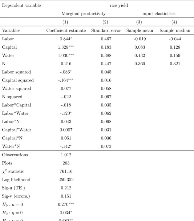
In this section, we check the relevance of the SFA model with our dataset. Here we specify the time-variant inefficiency as Battese and Coelli (1992). The inputs marginal productivity and elasticities are reported in Table 5.
Firstly, we check the theoretical consistency of our estimated efficiency model by ver-ifying that the marginal productivity of inputs are positive. If this theoretical criterion is met, then the obtained efficiency estimates can be considered as consistent with microe-conomics theory. As the coefficients of the translog functional form do not allow for direct interpretation of the magnitude and significance of any inputs, we compute the output elasticities for all inputs at the sample mean and median and report them in column (3) and column(4) 17.
In our sample, the paddy rice production in Sancha village depends more strongly on nitrogen (0.36) and water (0.13) at the sample mean. This suggests that the yield of rice production is most likely relative to nitrogen and water use. However, the marginal productivity of labor appears to be negative (-0.019) at the sample mean. This result seems to be relevant within the context of Chinese agriculture. According to other studies, surplus labor may exist in remote areas (Wan and Cheng, 2001; Fan et al., 2003). The over–use of labor inputs implies that the marginal productivity of labor must be very low, even negative in some cases (Tian and Wan, 2000; Tan et al., 2010; Chen et al., 2006). Finally, our results ensure that the returns to scale at sample mean and the sample median are both positive.
17The elasticities of mean output with respect to the jthinput variable are calculated at the mean of
the log of the input variable and its second order coefficients as follows: δlnY
δXj
Within the framework of the translog stochastic production frontier, we predict tech-nical efficiency scores and thereby calculate environmental efficiency scores (see Table 12 regarding descriptive statistics of both technical and environmental efficiency). Technical efficiency is significant in our sample with a mean value of 0.73, ranging from 0.33 to 0.98. The score suggests that most farmers, both conventional and organic, have sufficiently mastered the technology to produce satisfactory yield. However, when looking into the environmental efficiency scores, the mean value is only 0.45, ranging from 0.08 to 0.96. The standard error of environmental efficiency is higher (0.18) than that of technical ef-ficiency (0.12). This result suggests that most farmers are not environmentally efficient rather that technical efficiency cannot guarantee environmental efficiency. Should con-verting to organic farming help to improve environmental efficiency? We now turn to the second step of our analysis to investigate this question.
Table 5: Stochastic production frontier model
Dependent variable rice yield
Marginal productivity input elasticities
(1) (2) (3) (4)
Variables Coefficient estimate Standard error Sample mean Sample median
Labor 0.844∗ 0.467 -0.019 -0.044 Capital 1.328∗∗∗ 0.183 0.083 0.128 Water 1.030∗∗∗ 0.388 0.132 0.159 N 0.216 0.447 0.360 0.321 Labor squared -.086∗ 0.045 Capital squared -.164∗∗∗ 0.016 Water squared 0.077 0.058 N squared -.022 0.067 Labor*Capital -.018 0.035 Labor*Water -.120∗ 0.062 Labor*N 0.043 0.068 Capital*Water 0.0007 0.031 Capital*N 0.051 0.036 Water*N -.142∗ 0.073 Observations 1,012 Plots 203 χ2statistic 761.16 Log-likelihood 259.352 Sig-u (TE.) 0.212 Sig-v (errors.) 0.151 H0: µ = 0 0.270∗∗∗ H0: η = 0 0.034∗ H0: γ = 0 0.683∗∗
Estimation method: Maximum likelihood estimator with time-variant TE. H0: µ = 0, H0: η =
0 and H0: γ = 0 report alternatively the null hypotheses that the technical inefficiency effects
(1) have a half-normal distribution, (2) are time invariant and (3) present in the model. 5 seasons and 7 seeds are controlled for. *** statistical significance at 1%, ** statistical significance at 5%, * statistical significance at 10%.
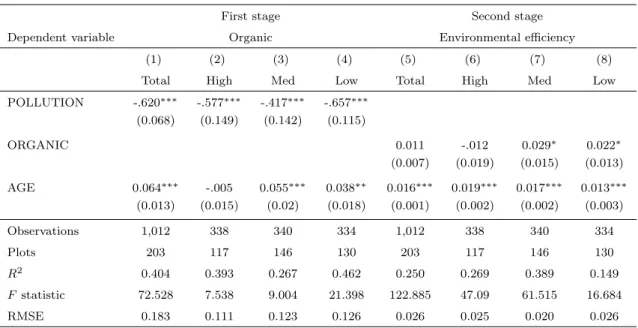
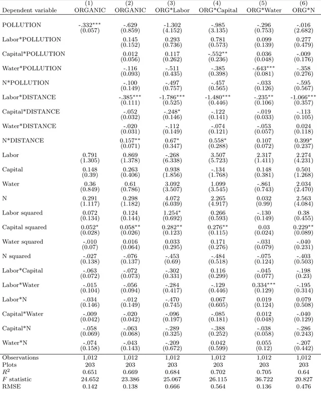
Table 6 presents the estimation results of equation 7. As discussed in Section 3.2, we explore the heterogenous effect of organic farming on different levels of nitrogen application by looking into three equal sub-samples. To save room, we only report results by the within-2SLS estimator and its first stage regression. The result of the within estimation are found in Table 14 in the Appendix.
Table 6: Environmental efficiency of organic farming
First stage Second stage Dependent variable Organic Environmental efficiency
(1) (2) (3) (4) (5) (6) (7) (8) Total High Med Low Total High Med Low POLLUTION -.620∗∗∗ -.577∗∗∗ -.417∗∗∗ -.657∗∗∗ (0.068) (0.149) (0.142) (0.115) ORGANIC 0.011 -.012 0.029∗ 0.022∗ (0.007) (0.019) (0.015) (0.013) AGE 0.064∗∗∗ -.005 0.055∗∗∗ 0.038∗∗ 0.016∗∗∗ 0.019∗∗∗ 0.017∗∗∗ 0.013∗∗∗ (0.013) (0.015) (0.02) (0.018) (0.001) (0.002) (0.002) (0.003) Observations 1,012 338 340 334 1,012 338 340 334 Plots 203 117 146 130 203 117 146 130 R2 0.404 0.393 0.267 0.462 0.250 0.269 0.389 0.149 F statistic 72.528 7.538 9.004 21.398 122.885 47.09 61.515 16.684 RMSE 0.183 0.111 0.123 0.126 0.026 0.025 0.020 0.026 Note: Robust standard errors in parentheses. Distance, sex and education are dropped given their time invariant nature. *** statistical significance at 1%, ** statistical significance at 5%, * statistical significance at 10%.
At first glance, the difference of environmental efficiency between organic and con-ventional farming is non-significant (Col.5). However, the picture is not the same for all sub-samples. At low and medium levels of nitrogen (i.e., application rate below 15.29 kg per mu), the sign of organic farming is positive at 10 percent statistical significance (Col.7 and 8). This means that for plots with medium and low nitrogen, converting to organic farming does minimize the nitrogen use at the actual output level. The advantage of organic farming is thus obvious compared to conventional farming. Nevertheless, this performance of organic farming does not sustain a high nitrogen level (i.e., application
rate above 15.29 kg per mu). The effect of organic farming becomes negative but non– significant (Col.6). In other words, for plots using high levels of nitrogen, converting to organic farming does not minimize the nitrogen application and thus does not allow for improvement in environmental efficiency.
This result is not surprising. In Europe, for instance, at high nitrogen application lev-els, agronomist experiments also provide evidence showing that the nitrogen-use efficiency of organic farming systems is indeed lower than conventional farming systems (Kirchmann and Ryan,2004). This result suggests that in a developing country like China, one should interpret the effect of organic farming with caution. Rapid conversion to organic farming does not necessarily mean the reduction of nitrogen use. At high levels of nitrogen in-put, conversion to organic farming does not improve environmental efficiency or resolve agricultural pollution problems due to nitrogen overuse.
5.4
Robustness check
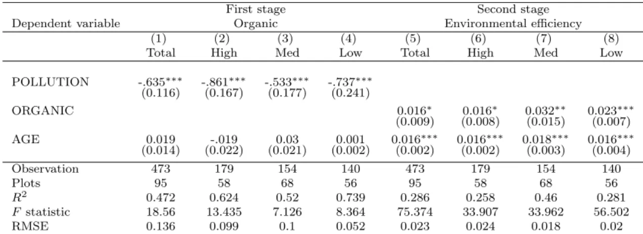
How to explain the decreasing performance of organic farming at high nitrogen levels? As mentioned in Section 2, newly converted farmers in Sancha village tend to use more nitrogen due to their uncertainty and lack of training. Meanwhile, the experience and field management capacity of farmers could also determine their environmental efficiency. Intuitively, the behaviors of newly converted farmers may probably explain the reduction of environmental efficiency for organic farming at high nitrogen levels. With our dataset, we can test this explanation by focusing on environmental efficiency of trained farmers, i.e., those who participated in the early organic farming experimentation in 2005. With the name list provided by the NGO, we are able to identify households who have participated in the experimentation and converted to organic farming since then. We redo the same estimation with observations of these households and check the results again. If the results turn out to be positive and significant for all sub-samples, we can then validate this explanation. We now turn to the within-2SLS estimation results in Table 7 (see the results of the within estimation in 15 in the Appendix).
efficiency regardless of the nitrogen level. This result confirms our explanation and com-pletes the story. Having received effective technical training and environmental education provided by the PCD, experienced farmers are indeed more conscious about the environ-mental problem and more respectful of the principles of organic farming. With effective training in farm management, they are able to minimize the use of external nitrogen rather than increasing it to maintain the output as done by newly converted farmers. From the environmental efficiency point of view, the organic farming conducted by trained farmers is more sustainable than that of newly converted farmers. Taken together, our results stress the importance of technical and institutional assistance in the promotion of organic farming. Effective support such as farmer capacity building and environmental education are indispensable in guaranteeing the environmental efficiency of organic farming in its development. Without this support, organic farmers may use more organic nitrogen to compensate for the lack of chemical fertilizer and ignore the management of nitrogen. As a result, while maintaining the output, organic farming may fail to achieve its objective of environmental protection.
Table 7: Environmental efficiency of trained organic farmers
First stage Second stage Dependent variable Organic Environmental efficiency
(1) (2) (3) (4) (5) (6) (7) (8) Total High Med Low Total High Med Low POLLUTION -.635∗∗∗ -.861∗∗∗ -.533∗∗∗ -.737∗∗∗ (0.116) (0.167) (0.177) (0.241) ORGANIC 0.016∗ 0.016∗ 0.032∗∗ 0.023∗∗∗ (0.009) (0.008) (0.015) (0.007) AGE 0.019 -.019 0.03 0.001 0.016∗∗∗ 0.016∗∗∗ 0.018∗∗∗ 0.016∗∗∗ (0.014) (0.022) (0.021) (0.002) (0.002) (0.002) (0.003) (0.004) Observation 473 179 154 140 473 179 154 140 Plots 95 58 68 56 95 58 68 56 R2 0.472 0.624 0.52 0.739 0.286 0.258 0.46 0.281 F statistic 18.56 13.435 7.126 8.364 75.374 33.907 33.962 56.502 RMSE 0.136 0.099 0.1 0.052 0.023 0.024 0.018 0.02 Note: Robust standard errors in parentheses. Distance, sex and education are dropped given their time invariant nature. *** statistical significance at 1%, ** statistical significance at 5%, * statistical significance at 10%.
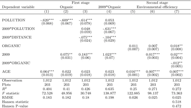
To check the robustness of our results, we explore the performance of organic farming over time. We recall that the boost of nitrogen input in organic farming is observed in the scale-up period from 2009 (see Table 2 in Section 2). As a consequence, a substantial number of newly converted organic farmers joined the organic farming project from 2009
environmental efficiency after 2009. The results can be found in Table 8.
Table 8 reports the environmental performance of organic farming before and after 2009 when the organic farming project scaled up. The results estimated by the within-2SLS estimator are presented and the results by the within estimator are found in Table 16 in the Appendix. In column 7, organic farming is found to have a positive and significant effect on environmental efficiency after controlling for both the turning point in the organic farming project, i.e., 2009, and plot fixed effects. However, the interaction term has a significant and negative effect. That is to say, before 2009, organic farming was more efficient than conventional farming in terms of environmental efficiency. However, after 2009, this environmental performance of organic farming significantly decreased. This result is in line with our previous findings and confirms the robustness of our result stating that newly converted organic farmers increased the use of external nutrients in an attempt to compensate for the potential yield loss they feared.
Table 8: Environmental efficiency of organic farming over time
First stage Second stage Dependent variable Organic 2009*Organic Environmental efficiency
(1) (2) (3) (4) (5) (6) (7) POLLUTION -.620∗∗∗ -.609∗∗∗ -.614∗∗∗ 0.053 (0.068) (0.067) (0.078) (0.069) 2009*POLLUTION 0.048 -.631∗∗∗ (0.059) (0.067) 2009*DISTANCE -.075∗∗∗ -.104∗∗∗ (0.024) (0.029) ORGANIC 0.011 0.007 0.018∗∗ (0.007) (0.007) (0.008) 2009 0.075∗∗ 0.183∗∗∗ 1.023∗∗∗ 0.017∗∗∗ 0.02∗∗∗ (0.031) (0.06) (0.07) (0.003) (0.004) 2009*ORGANIC -.012∗∗ (0.005) AGE 0.064∗∗∗ 0.022 0.023 0.023 0.016∗∗∗ 0.007∗∗∗ 0.007∗∗∗ (0.013) (0.019) (0.018) (0.018) (0.001) (0.002) (0.002) Observation 1,012 1,012 1,012 1,012 1,012 1,012 1,012 Plots 203 203 203 203 203 203 203 R2 0.404 0.41 0.426 0.635 0.25 0.271 0.272 F statistic 72.528 48.956 30.748 138.877 122.885 98.137 73.363 RMSE 0.183 0.182 0.18 0.198 0.026 0.025 0.025 Hansen statistic 0.518 Hansen P-value 0.472
Note: Robust standard errors in parentheses. Distance, sex and education are dropped given their invariant variables. *** statistical significance at 1%, ** statistical significance at 5%, * statistical significance at 10%.
6
Concluding remark and discussions
In this paper, we attempt to evaluate the sustainability of non-certified organic farming with respect to yield and external nitrogen utilization in the case of rice production in southern China. To this end, we estimate a classical SFA model and check the hypothesis of a “technology gap” between organic and conventional farming. Then we calculate the environmental efficiency scores for both systems from the estimated technical efficiency scores. We use these scores to measure the environmental performance (i.e., nitrogen management) of smallholder farmers. This exercise is useful to provide insight about non– certified organic farming’s environmental performance and to understand the condition for its sustainable development in developing countries. The data used for this exercise is derived from a plot-level household survey conducted in Sancha village where non-certified organic farming is rapidly expanding.
With this case study, we demonstrate several interesting results. First, conversion to organic farming does not necessarily reduce the rice yield if farmers can substitute chem-ical fertilizers with organic nutrients. There is no significant “technology gap” between organic and conventional farming in a smallholder environment. Second, nitrogen man-agement is not always optimal in an organic system, especially for newly converted organic farmers who lack training. At high nitrogen application levels, organic farming has no advantage in terms of environmental efficiency. In other words, to maintain the yield, organic farming consumes the same quantity, and sometimes more, of environmentally detrimental nutrients than conventional farming in developing country.
The experience of Sancha village has critical policy implications for non-certified or-ganic farming development in developing countries. By definition, oror-ganic farming is a kind of agricultural exploitation with long term objectives to preserve the environment. Its sustainability relies more on efficient nutrient cycling within the agro–ecosystem than on the external nutrient supply. The aim of nutrient application is thus to improve and enhance the fertility and resilience of soil, but not to feed the plants directly. Substitution
of chemical fertilizer by organic nutrients is a first step but is not sufficient to achieve this goal. Therefore, additional efforts such as technical support and environmental education are required for the control of nutrient application.
In developing countries, driven by political and economic interests, governments of-ten ignore this critical condition and promote organic farming solely through economic policies such as organic fertilizer subsidies. This economic policy appears effective as it reduces the cost of organic nutrients and encourages conversion in the short term. Nev-ertheless, it risks inducing rapid conversion and high organic nutrient application which can induce inexperienced farmers laking effective technical support to apply the same, or more, nutrients than conventional farmers in an attempt to maintain the yield. This policy is thus non sustainable in areas facing a shortage of organic nutrient supplies and nutrient surpluses in the soil. In light of growing trends that see governments seeking to expand and industrialize organic farming in developing countries, our study warns of the potential risk of rapid expansion, and highlights the need for regulation of nutrient application in developing countries.
In order to preserve the environmental efficiency of organic farming and develop it in a sustainable way, governments and development agencies need to provide more institutional support such as environmental education and technical training to accompany farmers during the conversion period. Otherwise, more strict regulation with respect to nutrient application is needed in the rapid expansion of organic farming in developing countries.
References
Avery, D. T., 1998. The hidden dangers of organic food. American Outlook, 19–22. Badgley, C., Moghtader, J., Quintero, E., Zakem, E., Chappell, M. J., Avil`es-Vaquez,
K., Samulon, A., Perfecto, I., 2007. Organic agriculture and the global food supply. Renewable Agriculture and Food Systems 22 (02), 86–108.
Battese, G. E., Coelli, T. J., 1992. Frontier production functions, technical efficiency and panel data: With application to paddy farmers in india. Journal of Productivity Analysis 3 (1-2), 153–169.
Battese, G. E., Coelli, T. J., Jun. 1995. A model for technical inefficiency effects in a stochastic frontier production function for panel data. Empirical Economics 20 (2), 325–332.
Battese, G. E., Rao, D. P., 2002. Technology gap, efficiency, and a stochastic metafrontier function. International Journal of Business and Economics 1 (2), 87–93.
Battese, G. E., Rao, D. P., O’Donnell, C. J., 2004. A metafrontier production function for estimation of technical efficiencies and technology gaps for firms operating under different technologies. Journal of Productivity Analysis 21 (1), 91–103.
Chen, Z., Huffman, W., Rozelle, S., 2006. Farm technology and technical efficiency: Evi-dence from four regions in china. Tech. Rep. 12605, Iowa State University, Department of Economics.
Christensen, L. R., Jorgenson, D. W., Lau, L. J., 1971. Conjugate duality and the tran-scendental logarithmic function. Econometrica 39 (4).
Connor, D. J., 2008. Organic agriculture cannot feed the world. Field Crops Research 106 (2), 187–190.
Cuesta, R. A., Lovell, C. K., Zofio, J. L., June 2009. Environmental efficiency measurement with translog distance functions: A parametric approach. Ecological Economics 68 (8-9), 2232–2242.
Day, A., 2008. The end of the peasant? new rural reconstruction in china. Boundary 2 35 (2), 49–73.
Fan, S., Zhang, X., Robinson, S., 2003. Structural change and economic growth in china. Review of Development Economics 7 (3), 360–377.
FAO, 2002. Organic Agriculture, Environment and Food Security. FAO.
Hessel Tjell, K., Aronsson, H., Torstensson, G., Gustafson, A., Linden, B., Stenberg, M., Rydberg, T., 1999. Dynamic of mineral n and plant nutrient leaching in fertilized and manured cropping systems with and without catch crop. results from a sandy soil in halland, period 1990-1998. Report no 50.
Hine, R., Pretty, J. N., Twarog, S., 2008. Organic agriculture and food security in Africa. United Nations.
Hossain, M., Elahi, S., White, S., Alam, Q., Rother, J., Gaunt, J., May 2012. Nitrogen budgets for boro rice (Oryza sativa l.) fields in bangladesh. Field Crops Research 131 (0), 97–109.
IFAD, Damiani, O., 2002. The Adoption of Organic Agriculture Among Small Farmers in Latin America and the Caribbean: Thematic Evaluation. International Fund for Agricultural Development.
Jia’en, P., Jie, D., 2011. Alternative responses to the modern dreamˆa ˇD´c: the sources and contradictions of rural reconstruction in china. Inter-Asia Cultural Studies 12 (3), 454–464.
Ju, X. T., Kou, C. L., Christie, P., Dou, Z. X., Zhang, F. S., Jan. 2007. Changes in the soil environment from excessive application of fertilizers and manures to two contrasting intensive cropping systems on the north china plain. Environmental pollution (Barking, Essex: 1987) 145 (2), 497–506, PMID: 16777292.
Kirchmann, H., Esala, M., Morken, J., Ferm, M., Bussink, W., Gustavsson, J., Jakobsson, C., 1998. Ammonia emissions from agriculture. Nutrient Cycling in Agroecosystems 51 (1), 1–3.
Kirchmann, H., Ryan, M. H., 2004. Nutrients in organic farming-are there advantages from the exclusive use of organic manures and untreated minerals. In: New directions for a diverse planet. Proceedings of the 4th international crop science congress. Vol. 26. Leibenstein, H., 1966. Allocative efficiency vs. x-efficiency. American Economic Review
56 (3), 392–415.
Mayen, C. D., Balagtas, J. V., Alexander, C. E., 2010. Technology adoption and technical efficiency: Organic and conventional dairy farms in the united states. American Journal of Agricultural Economics 92 (1), 181–195.
Mussgnug, F., Becker, M., Son, T., Buresh, R., Vlek, P., Aug. 2006. Yield gaps and nutrient balances in intensive, rice-based cropping systems on degraded soils in the red river delta of vietnam. Field Crops Research 98 (2-3), 127–140.
Oˆa ˘A´ZDonnell, C. J., Rao, D. P., Battese, G. E., 2008. Metafrontier frameworks for the study of firm-level efficiencies and technology ratios. Empirical Economics 34 (2), 231– 255.
OECD, 2001. Environmental Indicators for Agriculture: Methods and Results. OECD Publishing.
Pretty, J., Morison, J., Hine, R., Apr. 2003. Reducing food poverty by increasing agri-cultural sustainability in developing countries. Agriculture, Ecosystems & Environment 95 (1), 217–234.
Pretty, J. N., 1995. Regenerating agriculture: policies and practice for sustainability and self-reliance. Natl Academy Pr.
Pretty, J. N., Hine, R., 2001. Reducing food poverty with sustainable agriculture: A summary of new evidence. University of Essex UK.
Reinhard, S., Lovell, C. A. K., Thijssen, G., 1999. Econometric estimation of technical and environmental efficiency: An application to dutch dairy farms. American Journal of Agricultural Economics 81 (1), 44–60.
Renard, M., Guo, H., 2013. Social activity and collective action for agricultural innovation: a case study of new rural reconstruction in china. Cerdi Etudes et documents.
Sun, Bo, S. R.-P., Bouwman, A., 2008. Surface n balances in agricultural crop production systems in china for the period 1980-2015. Pedosphere 18 (3), 304–315.
Tan, S., Heerink, N., Kuyvenhoven, A., Qu, F., 2010. Impact of land fragmentation on rice producers technical efficiency in South-East china. NJAS - Wageningen Journal of Life Sciences 57 (2), 117–123.
Tian, W., Wan, G. H., 2000. Technical efficiency and its determinants in china’s grain production. Journal of Productivity Analysis 13 (2), 159–174.
Torstensson, G., 2003. Ecological farmingˆa ˘A¸S leaching and nitrogen turnover. cropping systems with and without animal husbandry on a clay soil in the county of vastergotland. period 1997-2002. Report no 73.
Twarog, S., 2006. Organic agriculture: A trade and sustainable development opportunity for developing countries. Trade and Environment Review, 141–223.
Wan, G. H., Cheng, E., 2001. Effects of land fragmentation and returns to scale in the chinese farming sector. Applied Economics 33 (2), 183–194.
Wang, G., Zhang, Q., Witt, C., Buresh, R., Jun. 2007. Opportunities for yield increases and environmental benefits through site-specific nutrient management in rice systems of zhejiang province, china. Agricultural Systems 94 (3), 801–806.
Wijnhoud, J., Konboon, Y., Lefroy, R. D., Dec. 2003. Nutrient budgets: sustainability assessment of rainfed lowland rice-based systems in northeast thailand. Agriculture, Ecosystems & Environment 100 (2-3), 119–127.
Willer, H., Rohwedder, M., Wynen, E., 2009. Organic agriculture worldwide: current statistics. The world of organic agriculture. Statistics and emerging trends, 25–58. WorldBank, 2009. World Development Report 2010: Development and Climate Change.
World Bank Publications.
Zhu, Y., Chen, H., Fan, J., Wang, Y., Li, Y., Chen, J., Fan, J., Yang, S., Hu, L., Leung, H., Mew, T. W., Teng, P. S., Wang, Z., Mundt, C. C., 2000. Genetic diversity and disease control in rice. Nature 406 (6797), 718–722.
Zhu, Z. L., Chen, D. L., 2002. Nitrogen fertilizer use in china: Contributions to food production, impacts on the environment and best management strategies. Nutrient Cycling in Agroecosystems 63 (2), 117–127.