Openness, Inequality, and Poverty: Endowments Matter

HAL Id: halshs-00557112

https://halshs.archives-ouvertes.fr/halshs-00557112

Preprint submitted on 18 Jan 2011

HAL is a multi-disciplinary open access archive for the deposit and dissemination of sci-entific research documents, whether they are pub-lished or not. The documents may come from teaching and research institutions in France or abroad, or from public or private research centers.

L’archive ouverte pluridisciplinaire HAL, est destinée au dépôt et à la diffusion de documents scientifiques de niveau recherche, publiés ou non, émanant des établissements d’enseignement et de recherche français ou étrangers, des laboratoires publics ou privés.

Openness, Inequality, and Poverty: Endowments Matter

Julien Gourdon, Nicolas Maystre, Jaime Melo De

To cite this version:

Julien Gourdon, Nicolas Maystre, Jaime Melo De. Openness, Inequality, and Poverty: Endowments Matter. 2011. �halshs-00557112�

CERDI, Etudes et Documents, E 2007.11

Document de travail de la série Etudes et Documents

E 2007.11

Openness, Inequality, and Poverty: Endowments Matter*

Revised April 20, 2007

51 p.

1

World Bank, University of Auvergne and CERDI: e-mail: Julien.Gourdon@u-clermont1.fr

2

University of Geneva: e-mail: Nicolas.Maystre@ecopo.unige.ch

3

University of Geneva, CERDI and CEPR: e-mail: DeMelo@ecopo.unige.ch

* We thank Jean-Marie Baland, Olivier Cadot, Marco Fugazza, Sylviane Guillaumont, Sébastien Jean, Jaya Krishnakumar, Alessandro Nicita, Branko Milanovic, Marcelo Olarreaga, Mathias Thoenig, Adrian Wood and seminar participants at UNCTAD (Geneva), T2M conference (Paris - PSE), the Universities of Milan and Namur for very helpful comments on an earlier draft. We also thank Branko Milanovic for providing us his WYD data set and answers to our numerous queries. An annex with detailed data sources and robustness checks is available from the authors upon request.

Abstract

Using tariffs as a measure of openness, this paper finds consistent evidence that the conditional effects of trade liberalization on inequality are correlated with relative factor endowments. Trade liberalization, measured by changes in tariff revenues, is associated with increases in inequality in countries well-endowed in highly skilled workers and capital or with workers that have very low education levels. Similar, though less robust, results are also obtained when decile data are used instead of the usual Gini coefficients. Taken together, the results are strongly supportive of the factor-proportions theory of trade and suggest that trade liberalization in poor countries where the share of the labor force with little education is high raises inequality. Simulation results also suggest that relatively small changes in inequality as measured by aggregate measures of inequality like the Gini coefficient are magnified when estimates are carried out using decile data.

JEL classification: F11, F16, D3

Keywords: International Trade, Income Distribution, Poverty.

Word count: 8604 Abstract: 144

1. Introduction

The relation between openness, inequality and poverty within countries continues to be subject to considerable controversy in the debate about globalization and in the academic

literature where the relative importance of the different transmission channels linking openness to inequality and poverty remains elusive. First, detailed case studies

decomposing the sources of the evolution of income inequality within countries reveal very different patterns across

countries. As to trade liberalization and openness--usually understood to mean the ease with which goods and services, factors of production (e.g. capital, labor and skills) move across countries as transaction costs fall-—they are often used interchangeably and captured by a trade-to-GDP ratio which captures many other features of a country’s exposure to trade. Second, whether from specific trade liberalization episodes or from cross-country studies, the evidence on the relation between trade liberalization and inequality is conflicting.1 Third, in most cross-country studies,

identification comes from cross-country variability in the inequality measure and no attempt is made to control for the source of the data on inequality.

If one were asked to point towards an emerging consensus, it would probably be that increasing openness has been

reflected in a growing wage gap between skilled and unskilled wages. Moving to the association between openness and overall

1 _{Bourguignon, Ferreira and Lustig eds. (2005, table 10.1) show the variety}

of underlying changes in inequality across four countries. Using four household surveys spanning the period of Mexican tariff liberalization, Nicita (2004) explores systematically the channels by which the Mexican trade liberalization affected households. He finds differential

pass-through effects across commodities and strong effects on spatial inequality and concludes that, overall, tariff liberalization might have been

associated with a reduction in poverty, but that inequality increased. Case study evidence is not considered further in this paper. Also see Galiani and Porto (2006) for a country study on trade liberalization and wage inequality in Argentina.

inequality (usually measured by the Gini coefficient) the evidence remains very mixed: many studies find no evidence of openness on inequality, or that openness increases inequality at all levels of development.2

More intriguing to many is the lack of robustness towards expectations from the standard factor-endowment-based trade model (Heckscher-Ohlin – HO for short): conflicting evidence that greater openness reduces (increases) inequality in

developing (developed) countries and very qualified support for the hypothesis that endowments matter along the expected lines (see below), not to mention little support for robust results between trade liberalization and inequality.3 The lack of correlation between factor endowments and inequality should also come as a surprise to scholars working on the

institutional foundations of development who generally find strong evidence that endowments matter in the evolution of a country’s inequality (Hoff (2004)).

Perhaps this should not come as a surprise and not concern us too much if, via other channels such as growth, increased openness reduces poverty. After all, HO theory should only be expected to inform us about the relation

between endowments and factor rewards in response to a reform-induced change in relative factor demands rather than between endowments and overall income inequality which is determined by many other factors. And, as pointed out by Baldwin (2004, p. 517) in his review of the trade liberalization and growth literature, since trade liberalization is rarely applied in isolation, it makes little sense to try and isolate its effects from those of associated policies.

2

Barro (2000), Lundberg and Squire (2003) and Milanovic (2005) find that openness increases inequality whereas Edwards (1997), Ravallion (2001) or Dollar and Kraay (2002) find no significant relationship.

3

See Anderson (2005) for a survey of the conflicting evidence on openness and inequality, and Winters et al. (2004) for a survey of the evidence on trade liberalization and poverty. Spilimbergo et al. (1999), Milanovic (2005) and Bensidoun et al. (2005) are the studies most closely related to ours.

In contrast to this agnosticism, following an exhaustive review of the evidence on trade liberalization and poverty, Winters et al. (2004, p. 108) conclude that trade

liberalization might be the easiest poverty-alleviating reform to accomplish, and the most powerful direct mechanism to

alleviate poverty in a country. If so, knowing more about the links between trade policy and inequality is important since, from a political-economy perspective, knowledge about the links between openness and inequality will inform about the feasibility of policies that increase openness and are likely to reduce poverty.

We bring new evidence on this issue using two data sets covering a larger sample of developing countries than most previous studies. We introduce fixed-effects (FE) so that identification of the effects of globalization is confined to variations in that country’s variables. We also broaden the range of control variables to address omitted variable bias. In this set up, we find rather consistently that trade

liberalization is associated with increases in inequality. Second, unlike most previous studies, we find that endowments matter along the lines suggested by the standard HO theory arguments reviewed in section 2. We find consistently that trade liberalization is associated with increases in

inequality in countries that are relatively well-endowed with capital and with highly skilled workers while it associated with decreases in inequality in countries relatively well-endowed in primary educated (unskilled) workers and in arable land. On the other hand, as suggested by Wood (1994, 2002), we find that trade liberalization is associated with increases in inequality in countries relatively well-endowed with workers lacking basic education.

The paper is organized as follows. Section 2 discusses the main channels linking openness and trade liberalization to inequality identified in the literature along with the two

data sets used in this paper. Using data over the period 1980-2000, section 3 establishes that the correlation between trade liberalization and inequality follows patterns predicted by factor-proportions theories. These results are largely

confirmed with a ‘high quality’ data set (based on deciles) covering the period 1988-98 in section 4. Section 5 concludes.

2. Transmission Channels and Data

2.1 Transmission Channels

The debate on the channels through which openness might affect inequality has largely revolved around the role of openness-induced changes in relative factor demands and their

consequent expected effects on factor rewards. For natural-resource-rich countries, though they do not deal directly with trade liberalization, Leamer et al. (1999), provide plausible scenarios and some evidence as to why the development paths of such countries could lead to rising inequality.

Concentrating on accumulable endowments where rent

effects should be minimal, Wood (2002) provides a convenient summary of the different channels via which globalization might affect wage inequality (see also Kremer and Maskin (2003)). As all forms of transaction costs fall with

globalization, factor mobility (capital via FDI and Northern K-workers in the terminology of Wood) is enhanced, leading to greater cooperation of Northern K-workers who travel to work with skilled workers in the South. In the South, workers with little or no-education (and hence low wages) would then be expected to be confined to non-traded activities. Trade liberalization would then not only lead to rising wages for skilled workers in the North and in the South, but under

plausible assumptions, it would also lead to an increase in wage inequality in the South.4

Feenstra and Hanson (1996) interpret globalization as an increase in FDI (rather than a movement of K-workers) leading to a rising volume of trade in intermediates (see Hummels et al. (2001) for supporting evidence) as the process of

production leads to a fragmentation of production. Again, in a HO framework where a continuum of intermediates are produced by the North and the South, and where the North is relatively well-endowed in skilled labor and capital (with capital and skilled labor complementary factors in production), Feenstra and Hanson, echoing Wood, show that an increase in FDI can lead to rising wages for skilled workers in the North and the South as FDI raises the skill-intensiveness of production in both countries.5

In reality, other channels beyond changes in factor rewards will affect inequality when a country becomes more outward-oriented. At the simplest level, in the Ricardo-Viner model changes in relative prices lead to changes in the

purchasing-power of households, and if the poor consume the exported good intensively, trade liberalization could increase income inequality. Several exercises using simulation models reported in Hertel and Winters eds. (2006) quantify the

potential magnitude of some of these channels, notably the

4

In a two-sector model (tradables and non-tradables) with capital and two categories of workers (skilled and unskilled), in which the three household categories are not diversified in their factor-ownership holdings and the unskilled are confined to the non-tradable sector, Bensidoun et al. (2005) show formally that an increase in the wage of skilled labor (brought about by increased openness) will increase the value of the Gini index if the share of unskilled labor is large enough.

5

Arguing that much trade is between rich countries and that much trade can be viewed as the production of a single product manufactured by outsourcing of components made and assembled in different countries, Kremer and Maskin (2003) develop a model in which globalization (again an increase in FDI) can plausibly lead to an increasing wage gap between skilled and unskilled workers in both the North and the South. The key mechanism in their model is that globalization leads to more cross-matching than self-matching (workers with the same skill levels working together).

poverty implications of tariff reductions on the purchasing power of households with different expenditure patterns.

More importantly, there are other context-specific transmission channels (see Winters et al. (2004) for discussion) which cannot be captured in a cross-country

exercise seeking to extract common elements that are likely to hold across a range of countries. For example, as shown by Nicita (2004) in his detailed case study of tariff

liberalization in Mexico during the 90s, price pass-through effects were substantially different across commodities, and the poverty effects of trade liberalization varied

substantially across regions.

2.2 Framework and Data

Using panel data, the literature has usually estimated a relation of the form:

0 1 it 1 it

it l it it

l

INQ =α +α Y +β OPEN +

∑

where INQ is the measure of inequality, _it Y is average income _it

per capita (either from the national accounts or from

household surveys), OPEN is a measure (eventually lagged to _it

control for endogeneity) that proxies for the country’s

outward-orientation6, and Z is a vector of control variables. _it

In the discussion above, there is no role for income as an explanatory variable. Its inclusion rests on some variant of a Kuznets-type relationship and for relative endowments, but also for structural changes (other than endowments but

including increased financial integration) that are associated with rising GDP per capita and could affect the transmission of globalization-related effects to households.

6 _{Greater outward-orientation goes beyond integration in goods markets. It}

includes integration in capital markets, as well as behind-the-border measures. Insofar as a reduction in transaction costs affect countries equally, these can be ignored. See further discussion below.

Note the absence of country fixed effects in (1). For example, in their widely-cited study examined below,

Spilimbergo et al.(1999) do not control for country-specific features that could account for differences in inequality such as labor market specificities emphasized by Rama (2002)),

productivity differences (see Easterly (2004)), or

institutions (Barro 2000). Nor do more recent studies (e.g. Milanovic (2005)) typically use such controls for

heterogeneity.7 Insofar as omitted factors do not change over time, the inclusion of fixed effects controls for such

idiosyncratic factors. Since our data set covers a rather long period, and inevitably some of the relevant omitted variables will change over time, this needs to be kept in mind when interpreting results. Likewise, the validity of the results rests on the assumption that the data reflect a sufficiently stable relationship (this is why we exclude all transition economies from our samples) and that the same dynamics can be imposed on all countries, an assumption that is less likely to hold, but about which little can be done.

We use two data sets. The first set of results is based on five-year average data spanning the 1975-2000 period

relying on the extensively used Deininger and Squire (D-S) data set (augmented to include the year 2000 by the

availability of the WIDER (2004) data). The second is the more recent high-quality data set World Income Distribution (WYD) also at approximately five-year intervals which covers the 1988-1998 period. Using two data sets provides further robustness checks, and the second data set is helpful when trying to quantify effects of trade liberalization on poverty. Table 1 shows that our sample has a good representation across

7

Among the studies that control for heterogeneity, Edwards (1997, 43 countries, 70s and 80s) finds no evidence that openness or trade

liberalization increases inequality. When including fixed effects, Barro (2000, 84 countries for 1960-90, table 6) finds no correlation between inequality and openness, echoing Ravallion’s correlations between average household incomes and inequality across 117 growth spells (Ravallion (2001), table 1).

regions, and that the developing countries are adequately represented.8

Table 1 here: Countries in the Sample

Regarding the variable used to capture a country’s outward-orientation, we use lagged tariffs i.e.TAR_{i t, −5}, (computed as the ratio of tariff revenues to imports) as a measure of trade openness. This is a more direct measure of openness than those often used previously (i.e. a trade output ratio, a ‘trade adjusted ratio’ obtained as a residual from an estimated relation of openness, or the Sachs-Warner index). As a consequence, our sample does not include the 1960-80 period covered in some of the earlier studies. Since most trade

liberalization in developing countries started in the early eighties, this may not be too damaging.

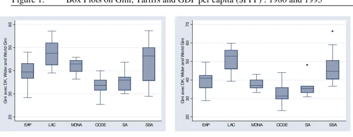
Figure 1 describes the main characteristics of the data at the regional level. The relative patterns of inequality remain unchanged across regional groupings, being the highest in Latin America and SSA throughout. Within regions, tariff dispersion fell and, except for the Middle East and North Africa (MENA) region, average tariffs declined during the sample period.

Figure 1 here: Box Plots on Gini, Tariffs and GDP per capita ($PPP): 1980 and 1995

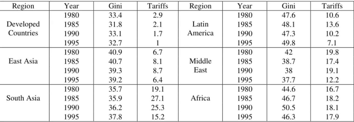
Table 2 gives regional averages for the two main

variables of interest, the inequality measure and our measure of openness, tariffs computed from customs data (see the annex for data sources and data manipulations). There is little

8

Only countries with economy-wide inequality measures (‘high-quality’ indices according to D-S) are retained in the sample. As a reference for comparison among the studies that concentrate on openness and inequality, the often-cited study by Spilimbergo et al. (1999) had 17 developed and 17 developing countries in their sample.

variation in the average measure of inequality within regions and persistent differences across regions while the measure of protection indicates (on average) a downward trend in all

regions except Africa. Since much of the trade reforms in the eighties often consisted of replacing NTBs with tariffs, what appears as an increase in protection could in fact represent either a reduction, or no increase in protection. In selecting tariffs as our measure of openness, we take refuge in the

often-made observation that the average tariff level is an adequate approximation of the restrictiveness of a country’s trade regime, and arguably less controversial than other measures often used, which in any event, are not available, over time (e.g. measures of NTBs).9 Of course, having a measure of tariff spreads across industries or between agriculture and manufactures would be helpful. Unfortunately such data are not available over time for a sufficiently large sample of

countries. However, as shown by Pritchett and Sethi (1994), because of widespread exemptions, tariff revenues do not

increase proportionately with tariff rates suggesting limited further information from having information on tariff spreads.

Table 2 here: Data on Inequality and Openness

We checked the correlation between our tariff measure for openness with other proxies often used. In general, the

correlation is rather weak, although reassuringly, the

correlation with the carefully constructed Wacziarg and Welch

9

According to Rodrik (2000), (p. 3): “Tariff and non-tariff averages are reasonably accurate in ranking countries in terms of trade policy openness, and in showing changes in openness over time”. Goldberg and Pavcnik (2004) reach the same conclusions and conclude that tariffs capture relatively well the combined effects of trade policy changes. They also note that the preoccupation about the endogeneity of tariffs is lessened by the fact that many countries moved towards a reduction in protection and more uniformity in their tariff structures when they became full members of the GATT/WTO. Moreover, the use of a synthetic index to measure the restrictiveness of a trade regime still has appeal especially during the 70s and 80s when many countries still had a multiplicity of trade barriers in their foreign exchange regimes.

(2003) index is quite high

(

ρ

)

strongest justification for using tariffs is their widespread availability and the likelihood that error measurements will be less than with other proposed measures.11

The main weakness in the data set is the absence of a measure of financial openness. Miniane (2004) provides a

summary of available indices of financial market integration. It turns out that even for the WYD data set which only covers the 1988-98 period, about 2/3 of the countries in our data set would not have a measure of financial market integration. We have therefore decided not to tackle the issue of financial market integration (using FDI as in e.g. Milanovic (2005), would not be appropriate since it is largely an outcome variable).

3. Trade Liberalization and Inequality: Endowments matter

We start exploring the basic HO prediction that trade liberalization should reduce inequality in low-income

countries and increase it in high income countries. Next, we bring in factor endowments which we interact with the tariff variable to isolate the effects of differing endowments on inequality. Throughout this section, the data covers the period 1980-2000 and the Gini coefficient is the inequality measure.

10

Unfortunately, for statistical analysis, the Wacziarg and Welch (2003) index is a binary variable. Tariffs are also strongly positively correlated [correlation coefficient in brackets] with other measures of trade barriers such as taxes on input and capital used by Barro & Lee (2002)[0.31]. Among the model-based estimates, tariffs are most closely correlated with the gravity-based index of Hiscox & Kastner (2002) [0.47] and the residuals from adjusted trade ratios estimated econometrically by Leamer (1987) [-0.43], but weakly with the Pritchett (1996) index [-0.08].

11 _{Because tariffs do not take into account NTBS, we also correlated several}

frequency indices of NTBs with our tariff measure at the HS-6 level using Jon Haveman’s treatment of TRAINS data. Correlations (available upon request) for different tariff ranges and the overall NTB frequency index ranges between 0.20 and 0.30 confirming high tariffs barriers are

3.1 Openness, Income and Inequality

We start with the traditional specification:

, 5 , 5 1 1 2 , 1,3 i=1,...,76, t=1,..., 4 ( * ) it i t i t it it i t it l it k ikt l k

INQ D YR Y TAR TAR Y

Z DS e

α

β

β

δ

γ

∑

∑

In(2), the index of inequality is regressed on a set of

country dummies D , a set of year dummies to control for any _i

common period shocks , on income per capita measured in PPP,

it

Y , tariffs (lagged one-period to control for endogeneity),

, 5

i t

TAR − , dummy variables, DS_ikt, to control for the source of

inequality data (dummy variables for gross vs. net income, income vs. expenditure, and households vs. individuals), and on a set of control variables,Z . All the variables are _it

expressed in logarithms.

As mentioned above, all data are five year averages (this helps to control for autocorrelation and measurement error), giving us up to four observations across time. The use of country fixed-effects reduces considerably the variance in inequality to be explained so that measurement errors are exacerbated even though taking five year averages should attenuate this problem (see Pritchett (2000)). Having more data points within countries, as in e.g. Galani and Porto (2006) who study the trade-liberalization wage-inequality relation in Argentina over thirty years would clearly be a superior identification strategy, but such an option is not yet in the cards.

Should an increase in openness (here lower values for

5

it

TAR ₋ ) raise inequality, it would be reflected in

β

HO) interpretation (with capital and labor as the sole

endowments) would call for

β

β

inequality with a turning point at 1

2

Y

β

β

= − .

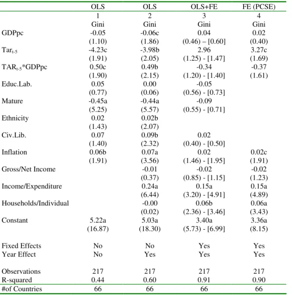
Estimates in table 3 column 1, with no fixed effects, correspond to those usually found in the literature (e.g. Barro (2000), Ravallion (2001), Rama (2002)). Under this

specification, trade liberalization raises inequality in poor countries, but reduces it in rich countries (i.e. with income per capita higher than 4,414$ PPP in column 1), in

contradiction with HO expectations. The estimates also indicate less inequality in low inflation countries and in countries with a higher share of population between 40 and 59 years old. The sign and coefficient estimates in column 1 are robust to the inclusion of year dummies (results not reported) which are included in the other estimates.

Insert table 3 here: Inequality, income and openness

Adding dummy variables for the source of income

inequality data in column 2 improves considerably the fit while increasing the significance of the coefficients

discussed above. In particular, the results contrary to HO predictions continue to hold at a higher (now 5%) level of significance (the turning point is now 3,600$). The signs on the dummies to control for the source of data on income

inequality have the expected: Gini coefficients based on

income (households) are higher than those based on expenditure (individuals). Our first finding is that all studies should control for the source of income inequality data (a point

already made by Ravallion (2001) and Bensidoun et al. (2005)). Since coefficient values on these dummies are always

to those reported here in tables 4 and 6, we do not comment on this result any further.

Column 3 introduces fixed-effects (FE) into the

estimation. Now, the sign of the coefficients for

(

β

β

)

(White) coefficients. Significance is slightly improved when we report panel-corrected standard errors in (these are in brackets in column 3) and borderline significance is reached in column 4 when insignificant variables are excluded.12 Our second conclusion is that results from studies that do not control for effects of omitted variables via FE are biased and that proxies for factor endowments effects behave according to expectations.13

This reversal between OLS and within estimates OLS can be understood from the data patterns in figure 1. Since the

richest countries (OCDE) have the smallest tariffs and the lowest level of inequality through time while SSA countries have the lowest income par capita, the highest tariffs and the highest level of inequality, a level estimation will show that countries with low tariffs and high income per capita will have the lowest income inequality. However, such a

relationship does not account for the impact of trade liberalization on inequality.

12

The Breusch Pagan test and the White test indicate heteroskedasticity in

the error process (σ2

it≠ σ2). We carried out our estimates using two

estimators: the standard heteroskedasticity-consistent White (1984) estimator and the panel-corrected standard errors (PCSEs) estimator

proposed by Beck and Katz (1995) which is shown to be as good or slightly superior to the robust estimator in Monte-Carlo studies for small samples (see Beck and Katz (1996, table 2). Since both estimators give very similar results, in subsequent tables we only report results based on PCSEs.

Ethnicity is dropped from the FE estimates because it is time-invariant.

13

Since we are mostly interested in endowments (which are all strongly correlated with income), we have not attempt to control for the endogeneity of income when estimating (3).

Changes in inequality could be due to the effects of other ongoing reforms such as concurrent stabilization policies. For example, Wacziarg and Welch (2003) show that trade liberalization often occurs during periods of systemic reforms including macro stabilization. Stabilization--here proxied by a reduction in inflation--is associated with a reduction in inequality (as in e.g. (e.g. Dollar and Kraay (2002), Edwards (1997)). However, including this control does not alter the relationship, nor does the introduction of other control variables that carry the expected signs.14

3.2. Trade Liberalization, Endowments, and Inequality

We now introduce relative endowments directly (rather than using income per capita as a proxy) interacting them with the openness measure as in previous studies (e.g. Bourguignon and Morrisson (1990), Spilimbergo et al. (1999) and Fisher

(2001)). This allows us to test whether the conditional

correlation of protection on inequality is sensitive to factor endowments. Results are reported in table 4.

5 1 1 1,6 5 * 2 1,6 1,3 ( ) it it i t m imt m it it m imt l it k ikt m l k INQ D YR TAR RE TAR RE Z DS e

β

φ

φ

δ

γ

∑

∑

∑

∑

As suggested by factor-endowment-based theories, relative endowment ratios,RE_imt, are computed relative to the

14 _{Ethno-linguistic fragmentation and less civil liberties increases}

inequality; financial depth and a high share of mature worker both reduce inequality. Spurious correlation from omitted variable bias could still be present. For example, trade liberalization could increase investment (see evidence in Wacziarg and Welch (2003)) which in turn could be correlated with inequality. Barro (2000) finds little correlation between inequality, and growth and investment in his sample, but Lundberg and Squire (2003) find support for a link in a simultaneous examination of inequality and growth.

corresponding sample mean per capita endowment.15 The ratios are weighted by the trade share in GDP to account for the endowments of closed countries that do not compete in the world markets with other factors (to help comparisons, we use the formula in Spilimbergo et al. (1999), see annex A4).

Since when we included fixed effects, most of the control variables,Z that vary little over time lost significance, so _it

we start by including only inflation and the dummies for the source of inequality data, both of which keep the same signs and significance levels as in columns 4 and 5 of table 3. Here with factor endowments entering directly in the specification, we are particularly interested in the values of the

interaction coefficients,

φ

We include six endowments. Labor is broken down into three categories along the lines suggested by the discussion in section 2 and indicated in (3): non-educated labor, i.e. those who have never been to school or have not completed primary school (NO); primary-educated or labor with a basic education (BS); and those that have an education level beyond high-school (SK). Such a breakdown suggested by the discussion

15 _{We also constructed relative endowments using trading partner countries}

as weights. Results were largely unaffected and are not reported here.

16

As a first exercise, not reported here, we replicated the same

specification as Spilimbergo et al. (1999) confirming their results (i.e. a result in conformity with factor-endowment predictions for human capital but in contradiction with predictions for physical capital when using their openness variable (‘adjusted’ trade ratio instead of tariffs). However, when using our preferred measure tariffs, increases in inequality are associated with relatively abundant endowments in capital following a reduction in tariffs (i.e. the coefficient on the interaction between relative endowment in capital per unit of labor, K/L, and the lagged tariff, is negative). To our knowledge, this plausible set of results has not been found in previous studies. However, with tariffs, the significance for the human capital endowment interactive term with tariffs disappears.

in section 2, was carried out recently by Bensidoun et al. (2005) in a slightly different context.17,18

Insert table 4 here: Inequality, factor endowments and openness

As to remaining endowments, Wood (2003) suggests that arable land per worker (AT/L) (as in Spilimbergo et al. (1999), Fisher (2001) or Leamer et al. (1999)) is not

sufficient to encompass natural resources and suggests using land per worker (T/L). Whereas arable land per worker captures factor intensities in the production of food and raw

materials, it does not include mining and fuels which are the less equally-distributed resources. This may explain why

several studies find that a strong endowment in arable land is associated with increases inequality during trade

liberalization (Spilimbergo et al. (1999) and Perry and

Olarreaga (2006)). Thus we use a direct measure of endowments in mining and fuels MF/L (captured by production in minerals, fuels and coal), next to the measure of arable land.

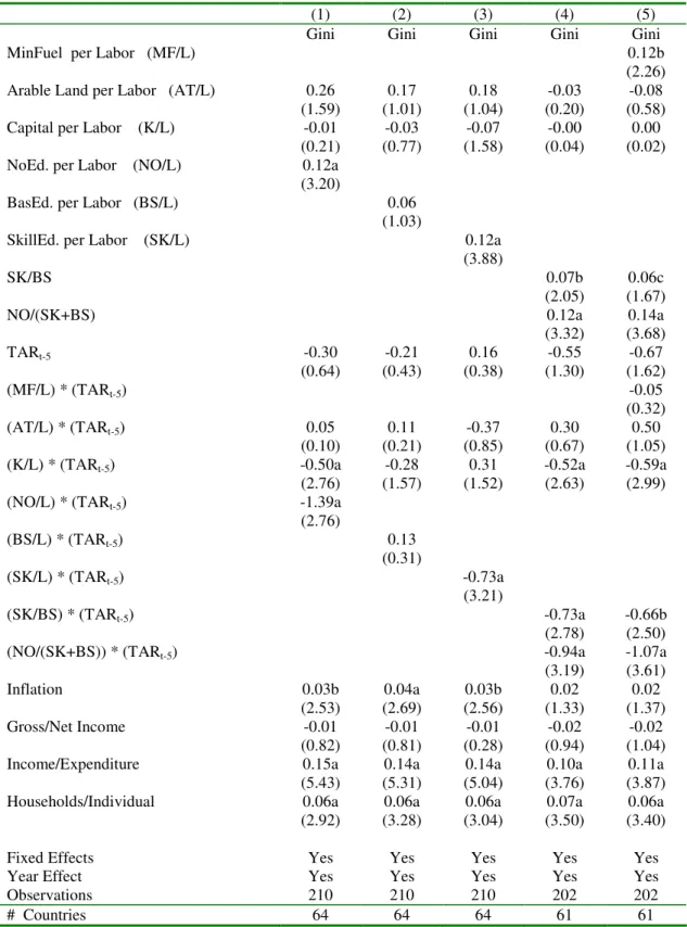
The first three columns of Table 4 test the significance of endowments relative to labor. Column 1 confirms the

expectation that trade liberalization in countries with

relatively high endowments in K/L and NO/L is associated with

17

Bensidoun et al. (2005) argue that the Heckscher-Ohlin model is too

restrictive, relying on factor-price-equalization (FPE) and hence identical production techniques in equilibrium. Using a more general approach that relaxes the FPE assumption (but still relies on other restrictive

assumptions like homothetic preferences and unchanged production techniques following trade liberalization), they show that factor price changes are correlated with the factor content of trade, leading them to test their model using constructed estimates of the labor-capital content of net exports instead of factor endowments on a similar D-S inequality data set for 53 countries. However, their results are not strictly comparable with ours (different sample with no SSA countries and a different definition of variables).

18

The index of human capital endowment (average years of schooling) is now replaced by these three different categories of skill levels. We take the NO variable from the Barro and Lee (2000) data set which is available on a five-year basis that corresponds to the 5-year averages used for all our variables.

a greater increase in inequality (negative coefficients for both interaction terms with lagged tariffs). Column 2 results also conform with factor endowment predictions since the

coefficient on BS/L interacted with lagged tariffs is

positive, but the K/L interaction term loses significance. The same expected pattern also holds in column 3 with SK/L.19 The result that trade liberalization is associated with greater increases in inequality in countries abundant in highly-educated labor is consonant with Galiani and Porto’s (2006) identification of an increasing skill premium in periods of trade liberalization in Argentina.

Column 4 controls for the skill composition of the labor force by including these three levels of education in ratio form to avoid perfect multicollinearity with the country

dummies: SK/BS, SK/L, and NO/(SK+BS).20 One can verify that, as predicted by factor endowment trade theories, during a trade liberalization, countries with a relatively (to the sample average) strong endowment in SK/BS experience a greater increase in inequality, while, after having controlled for skill endowments, countries relatively poorly endowed in labor with some qualification (i.e. with high values of NO/(SK+BS) experience an increase in inequality during a trade

liberalization. Column 5 shows that the proxy for mineral resources is associated with increases in inequality (as is a relatively strong endowment in SK/BS and in NO/(SK+BS)). In sum, globally the results in table 4 are supportive of factor-based predictions in almost all cases.

Table 5 quantifies the effects of a 5 percentage points reduction in tariffs on Gini coefficient value for different quartiles of the distribution of endowments. As, an example, tariff reduction increases the value of the Gini coefficient

19 _{Owing to the high correlation between SK/L and K/L}

(

_ρ

)

coefficient on K/L changes sign and is almost significant statistically.

by 0.4% for countries in the bottom quartile of the

distribution of (K/L), while it increases inequality by 6.0% for those in the top quartile. A similar pattern holds for (SK)/(BS), with the strongest effect for the ratio

(NO)/(SK+BS). Since countries with a high share of

non-educated population are also likely to be poorly endowed in capital, the two effects almost cancel each other.

Insert table 5 here: Tariff Reduction, inequality and factor endowments (see table A7b for full results).

We carried out several robustness checks. First, adding income (which serves as a proxy for omitted variables that would

exert an influence on inequality during trade liberalization) is not significant and does not alter the results above.

Likewise, including several macroeconomic and institutional variables largely preserves those results (and the included macroeconomic variables often have the predicted signs,

sometimes at statistically significant levels). For example, an improvement in civil liberties or an increase in government expenditure is associated with decreases in inequality (see results in table A6). Second, similar results are obtained when we apply our preferred specification to quintile data from the WIDER database (45 countries instead of 61). Results are reported in table A7. Third, in the absence of plausible instruments for tariffs which might be endogenous21, we test for reverse causality by regressing inequality on future rather than past tariffs, the results become mostly

insignificant suggesting that reverse causality is not a

problem. Fourth, the results are also robust to the exclusion of a small number of observations signaled as outliers by a

21

Using past values of differences in tariffs as an instrument makes little sense. Moreover, the average length of our sample (3.3 periods) makes it unsuitable for GMM estimations.

test on residuals. The pattern of signs is also broadly

similar when we exclude one region at a time (see table A8). Finally, we replaced tariffs with alternative indices of trade liberalization (see results in table A9). The sign (and often the significance) of our interactions terms are robust to the use of various trade ratios (see columns 2, 3 and 4). However, when we use the openness measures of Hiscox and Kastner

(2002), Spilimbergo et al. (1999), and Pritchett (1996), few coefficients of the interaction terms remain significant, although the signs remain the same (except in 4 cases). Overall, the results are moderately robust to alternative openness measures.

4. Openness, Inequality and Poverty: Further Results

Arguably, in spite of controls for the type of survey, the data set used so far is of lesser quality than the more recent World Income Distribution (WYD)22 data set that is drawn almost entirely from household surveys thereby allowing us to define welfare aggregates and recipient units consistently across countries and time. The WYD data set which also

provides information on income levels by deciles presents two advantages. First, it allows us to check for the robustness of our results in general, and also to the choice of inequality measure since we can work directly with decile data. Second, it is more appropriate to carry out estimates of the effects of trade liberalization on inequality and especially on

poverty, both because the quality of the data is presumably higher, but also because the calculations can also be carried out directly from the household sample mean income per

capita,m , rather than from GDP per capita from national _it

accounts.

22 _{WYD can be downloaded from}

Indeed, it has been argued that income measures from household survey data that is representative of the entire economy is a more reliable estimate of GDP than the

corresponding measures from the national accounts. In

particular, even though survey-based estimates of income have their own problems, Deaton (2005, p.18) argues that: “If we need to measure poverty in a way that will convince those who are skeptical of the idea that average growth reaches the

poor, there is little choice but to use the surveys”.23 In our sample the correlation between annual income growth over 1988 and 1998 measured from the surveys,g_H, and its equivalent from national income,g_PPP, is surprisingly low, (ρ=0.2917).

Moreover regressing g_H on g_PPP gives (std. errors in

parenthesis): 2

(0.357)

0.029 0.706 ; 0.0851

H PPP

g = + g R = .

Following the approach and specification in (3), we regress the share of the j-th decile in country i,

θ

with TAR_{i t, −5},and a set of controls (Zit) including country and

time dummies leading to the following equation to be estimated for each decile24:

, 5 1 1 1 1,3 , 5 * 2 1,3 ( ) ijt it i t ij i t j j m imt m it i t ijt m imt j l ilt it m l y D YR m TAR RE m TAR RE Z DS e θ α β φ φ δ − = − = ≡ = + + + + + + + +

∑

∑

∑

Table 6 reports the results for the bottom three and top three deciles (full results available in table A11).

23 _{See Deaton (2005) for a deeper discussion on this issue.}

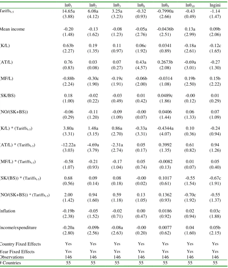
Insert table 6: Inequality (by decile), factor endowments and openness

Besides plausible estimates with the FE estimator (Milanovic (2005, footnote 8 argues that because this panel is very short there is insufficient data variability to use such an

estimator), the following patterns stand out. First, in spite of an insignificant correlation between GDP growth and sample mean income growth rates, the previous results hold over this sample period when using the Gini (or Theil) index as a

measure of inequality. (Signs in column 7 of table 6 are the same as those in table 4 and, with the exception of

K/L,significance holds for the interaction terms between tariffs and relative endowments.)

Turning to the decile estimates, by and large the same patterns continue to hold (remember the signs of the

coefficients should be reversed in columns 1 to 3 (when compared with those in columns 7). We still find that a reduction in protection decreases the share of the lower

deciles and that this effect is more pronounced for countries that have a high K/L ratio while the opposite holds for

countries with a high arable land (AT/L) ratio. However, when it comes to breaking down skills, the results lose

significance suggesting a lack of robustness when a finer breakdown of skills is attempted. While this should not be surprising since there is quite a high correlation across different endowment measures. Given the small time dimension, lack of controls and noise in the data, it is rather

comforting that the signs are preserved and near significance for the measure of the non-educated.

These results were submitted to several robustness checks (see tables in the appendix; others available upon request). First, we ran the same regression without taking the logarithm of the variables, obtaining similar results. Regarding reverse

causality, as previously, we ran the same regression using future trade rather than past values and the results become mostly insignificant, suggesting that reverse causality should not be a problem here. As to control variables, in other

specifications, we added government expenditure and/or an index of democracy, resulting in a large reduction in sample size. In general, the significant results in table 6 carry on to this smaller sample (see table A11).

Since the correlation between tariff reductions and inequality after controlling for endowments is still

significant in this shorter time span, we used the coefficient estimates in table 6 to simulate the average impact of a 5 point decrease in tariffs (this corresponds to the average tariff reduction during that period) on the bottom and top three deciles for two aggregated developing ‘regions’: Latin America (15 countries) and East, South and South East Asia (11 countries excluding Japan & Singapore).25 In each case,

regional values are values averaged over countries in the region26 and only statistically significant coefficients are used which means that the simulations mostly capture the estimated effect of differences in K/L and AT/L ratios.

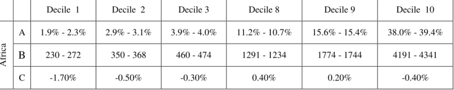
Results of this simulation exercise are reported in table 7.

Insert table 7: Decile changes in income simulated from a 5 percentage points reduction in tariffs

Subject to the validity of imposing the same reaction to tariff liberalization across countries, trade liberalization reduces the income of the first three deciles (and mildly up to decile 7) with usually a small increase for the top three

25 _{In a previous draft we also included SSA as a region. However, SSA only}

has 10 observations spread over 5 countries, implying a very unbalanced panel with only two observations per country.

26

Because of the possibility of outliers and influential observations, we checked that the results in table 6 were not sensitive to the exclusion of outliers.

deciles. Regarding the interpretation of the growth that would be necessary to compensate for the adverse effect of trade liberalization on income inequality, Wacziarg and Welch (2003) report an increase in average yearly growth (over a 7-year period) of 0.5 percentage points following the trade

liberalizations in their sample suggesting that the growth-induced effects of trade liberalization would not be

sufficient to compensate for the adverse distributional implications for the poorest quintile.

Finally, the often-observed lack of sensitivity of aggregate measures of inequality to changes in the

distribution of income is confirmed when inspecting the changes in the values of the Gini coefficients reported in table 7 (in spite of the large changes in mean decile incomes, Gini coefficient values only change at the third decimal). Because of the many biases likely to remain in these estimates in spite of the inclusion of many control variables, it is difficult to comment with confidence on the additional information provided by the detailed results on the decile data.

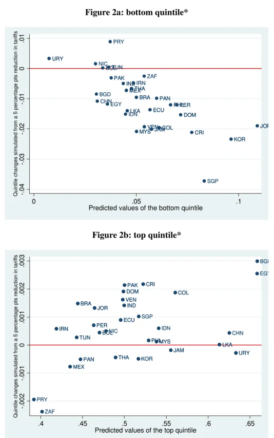
As an alternative presentation of these orders of magnitude, figure 2 reports country-level estimates of the simulated changes in the bottom and top quintiles of the distribution.27 Gains and losses in the bottom quintile are mostly reflected in changes in the top quintile rather than the middle of the distribution.

Insert figure 2: Simulated changes in quintile mean incomes of a 5 percentage points reduction in tariffs

27 _{The simulations are based on average values over the period. Because of}

the inclusion of fixed effects in our estimations, actual values of mean quintile shares are extremely close to those reported in figure 2,

5. Conclusions

Much of previous research on the correlates of inequality has established that inequality is largely determined by

factors that are quite different across countries and that change only slowly within countries. Notably, the effects of changes in trade policies, and of globalization more

generally, have been difficult to detect. This paper has focused exclusively on within-country variations to trade policy changes while carefully disaggregating factor

endowments. Overall, the results suggest that changes in inequality are correlated with changes in tariffs which are quite robust to inclusion of various controls and to changes in sample periods.

Several patterns emerge from these conditional

correlations that support the usefulness of resorting to factor-proportions theories of international trade when studying the effects of changes in trade policy on income distribution.

First, along Stolper-Samuelson predictions, with income per capita serving as a proxy for factor endowments, trade liberalization is associated with an increase in inequality in high-income countries and a decrease in inequality in

low-income countries, a result that has escaped most previous

studies that have neglected to distinguish within-country from between-country effects.

Second, after accounting for several controls, when interacted with tariffs, factor endowments have the expected effects on inequality. Trade liberalization is associated with increases in inequality in capital-abundant and high-skill abundant countries. Increases in inequality are also

positively correlated with trade liberalization in countries abundant in a non-educated labor force, though it decreases inequality in countries that are well-endowed with

primary-educated labor. These results give support to the critics of globalization who often point out that trade liberalization in poor countries leads to increases in inequality.

While spurious correlation cannot be excluded, this

result on the pattern of signs is quite robust to the addition of several control variables which also carry expected signs. We find no evidence of reverse causality. Controlling for the sources of income distribution data is almost always

significant along expected lines. A reduction in macroeconomic instability (proxied by a reduction in inflation) also reduces within-country inequality.

More tentative conclusions are reached when it comes to the extending the analysis of distributional shifts by

studying the whole income distribution rather than using aggregate distribution measures like the Gini or Theil coefficients. Over a shorter ten-year time-span, we obtain similar results with decile data, but the estimates often lack precision when we attempt to break down factor endowments

beyond capital and labor to include skill and education levels. Nonetheless, even though measurement errors are

probably exacerbated by the short temporal dimension, we would maintain that the relative robustness of the endowment effects to changes in specification justifies looking beyond averages and quantifying effects on the poor.

References

Anderson, E. (2005). "Openness and Inequality in Developing Countries: A Review of Theory and Recent Evidence", World

Development, vol. 33(7), pp. 1045-1063.

Baldwin, R.E. (2004). “Openness and Growth: What’s the

Empirical Relationship” chp. 13 in R.E. Baldwin and A. Winters eds. Challenges to Globalization: Analyzing the Economics, The University of Chicago Press.

Barro, R. (2000). “Inequality and growth in a panel of countries”, Journal of Economic Growth, vol. 5, pp. 5-32. Beck, N. and J.N. Katz (1995), “What to do (and not to do) with Time-Series Cross-Section Data”, The American Political

Science Review, 89(3), 634-47.

Beck, N. and J.N. Katz (1996), “Nuisance vs. Substance:

Specifying and Estimating Time-Series Cross-Section Models”,

Political Analysis, 1-36.

Bensidoun, I., S. Jean and A. Sztulman (2005). “International Trade and Income Distribution: Reconsidering the Evidence”,

CEPII Working Paper No.2005-17

Bourguignon, F. Morrisson, C. (1990). "Income Distribution Development and Foreign Trade", European Economic Review, vol. 34(6), pp. 1113-1133.

Deaton, A. (2005) "Measuring Poverty in a Growing World (or Measuring Growth in a Poor World)" The Review of Economics and Statistics, MIT Press, vol. 87(2), pages 395-395.

Deininger, K. Squire, L. (1996). "A New Data Set Measuring Income Inequality", World Bank Economic Review, vol. 10(3), pp. 565-592.

Dollar, D. and A. Kraay (2002). “Growth is Good for the Poor”,

Journal of Economic Growth, vol. 7, pp. 195-225.

Edwards, S. (1997). "Trade policy, Growth and Income

Distribution", American Economic Review, vol. 87(2), pp. 205-210.

Feenstra, R. Hanson, G. (1996). "Foreign Investment,

Outsourcing and Relative Wages" in R. Feenstra, G. Grossman and D. Irwin eds.,The Political Economy of Trade Policy: Essays in Honor Jagdish Bhagwati, MIT Press Cambridge.

Fisher, R. (2001). "The Evolution of Inequality after Trade Liberalization", Journal of Development Economics, vol. 66, pp. 555-579.

Galiani, S., and G. Porto (2006), “Trends in Trade Reforms and Trends in Wage Inequality”, WPS# 3905, World Bank.

Goldberg, P. and N. Pavcnik (2004). "Trade, Inequality, and Poverty: What Do We Know? Evidence from Recent Trade

Liberalization Episodes in Developing Countries", NBER Working

Paper No. W10593, June.

Hiscox, M.J. Kastner, S.L. (2002). “A General Measure of Trade Policy Orientations: Gravity Model-Based Estimates from 83 nations, 1960 to 1992”, UCSD working Paper 2002J.

Hertel, T., and L. A. Winters, eds. (2006), Poverty and the

WTO: Impacts of the Doha Development Agenda, Palgrave McMillan

and the World Bank

Hoff, K. (2004) “Paths of Institutional Development: A View from History”, mimeo, World Bank.

Hummels, D., J. Ishii and K-M. Yi (2001). “The Nature and Growth of Vertical Specialization in World Trade”, Journal of

International Economics, vol. 54(1), pp. 75-96.

Kremer, M. and E. Maskin (2003). “Globalization and Inequality”, (mimeo)

Leamer, E. Maul, H. Rodriguez, S. Schott, P.K. (1999). "Does Natural resources abundance increase Latin American income inequality?", Journal of Development Economics vol. 59, pp. 3-42.

Milanovic, B. (2005). “Can we discern the effect of

globalization on income distribution: evidence from household surveys”, World Bank Economic Review.

Milanovic, B. (2005a). Worlds Apart: Global and International Inequality 1950-2000, Princeton University Press.

Miniane, J. (2004), “A New Set on Capital Account Restrictions”, IMF Staff Papers, 81(2),

Nicita, A. (2004). “Who Benefited from Trade Liberalization in Mexico? Measuring the Effects on Household Welfare”,

Perry, G. and M. Olarreaga (2006), “Trade Liberalization, Inequality and Poverty Reduction in Latin America”, Mimeo, World Bank

Pritchett, L. (1996), "Measuring Outward Orientation in LDCs: can it be done?", Journal of Development Economics, vol. 49, pp. 307-335.

Pritchett, L., (2000), "Understanding Patterns of Economic Growth: Searching for Hills Among Plateaus, Mountains and Plains", World Bank Economic Review, vol. 14(2), pp. 221-50. Pritchett, L. and G. Sethi (1994), “Tariff Rates, Tariff

Revenue, and Tariff Reform: Some New Facts”, World Bank

Economic Review

Rama, M. (2002), "Globalization, Inequality and Labor Market Policies", Revue d’Economie du Développement, vol. 1-2, pp. 43-84.

Ravallion, M. (2001). "Growth Inequality and Poverty: Looking Beyond Averages", World Development, vol. 29(11), pp. 1803-1815.

Rodrik, D. (2000). “Comments on ‘Trade, Growth, and Poverty’ by D. Dollar and A. Kraay”, draft. Available at

http://ksghome.harvard.edu/~.drodrik.academic.ksg/

Spilimbergo, A. Londono, J.L. Székely, M., (1999). "Income distribution, factor endowments, and trade openness", Journal

of Development Economics, vol. 59, pp. 77-101.

Wacziarg, R. and K. H. Welch (2003). "Trade Liberalization and Growth: New Evidence", NBER Working Papers 10152, National Bureau of Economic Research, Inc.

Winters, A. McCulloch, N. McKay, A. (2004). “Trade

Liberalization and Poverty: The Evidence So Far”, Journal of

Economic Literature, vol. 42, pp. 72-115.

White, H. (1980), “A Heteroskedasticity-consistent Covariance Matrix and a Direct Test for Heteroskedasticity”,

Econometrica, 48:817-38.

Wood, A. (1994). North-South trade employment and inequality, Oxford University Press, Clarendon

Wood, A. (1997). "Openness and Wage Inequality in Developing Countries: The Latin American Challenge to East Asia

Conventional Wisdom", World Bank Economic Review, vol. 11(1), pp. 33-57.

Wood, A. (2002). "Globalization and Wage Inequalities: A

Synthesis of Three Theories", Weltwirtchafliches Archiv, vol. 138(1), pp. 54-82.

Wood, A. (2003), “Could Africa be Like America”, in B.

Pleskovic and N. Stern eds, ABCDE: The New Reform Agenda, pp. 163-200.

Tables to

Trade Liberalization, Inequality, and Poverty: Endowments Matter by

Julien Gourdon, Nicolas Maystre, Jaime de Melo

Table 1: Countries in the samplea

Sample for the study on 1980-2000 Sample for the study on 1988-1998

Regions Number of countries Number of obs. Number of countries Number of obs.

Developed 20 66 19 51

Africa & Middle East 14 42 10 23

Asia 10 36 11 29

Latin American 17 54 15 43

Total 61 198 55 146

Notes: List of countries is reported in Annex 1 and 2.

a

Transition and ex-USSR countries are excluded. Countries with less than two observations are also dropped from the sample

Table 2: Data on Inequality and Openness

Table 2: Inequality and Tariffs

Region Year Gini Tariffs Region Year Gini Tariffs

1980 33.4 2.9 1980 47.6 10.6 1985 31.8 2.1 1985 48.1 13.6 1990 33.1 1.7 1990 47.3 10.2 Developed Countries 1995 32.7 1 Latin America 1995 49.8 7.1 1980 40.9 6.7 1980 42 19.8 1985 40.7 8.1 1985 38.7 17.4 1990 39.3 8.7 1990 38 19.1 East Asia 1995 39.2 6.4 Middle East 1995 37.7 12.2 1980 35.7 19.1 1980 44.6 16.7 1985 35.9 27.1 1985 46.7 18.2 1990 36.2 25.3 1990 50.5 18.1 South Asia 1995 37.8 15.2 Africa 1995 46.3 17.9

Figure 1: Box Plots on Gini, Tariffs and GDP per capita ($PPP) : 1980 and 1995 2 0 3 0 4 0 5 0 6 0 G in i a v e c D K , W id e r a n d W o rl d G in i

EAP LAC MONA OCDE SA SSA

2 0 3 0 4 0 5 0 6 0 7 0 G in i a v e c D K , W id e r a n d W o rl d G in i

EAP LAC MONA OCDE SA SSA

Gini: 1980 Gini: 1995 0 1 0 2 0 3 0

EAP LAC MONA OCDE SA SSA

0 1 0 2 0 3 0 4 0

EAP LAC MONA OCDE SA SSA

Tariffs: 1980 Tariffs: 1995 6 7 8 9 1 0 G D P p e r c a p it a

EAP LAC MONA OCDE SA SSA

6 7 8 9 1 0 1 1 G D P p e r c a p it a

EAP LAC MONA OCDE SA SSA

Table 3: Inequality, income and openness

OLS OLS OLS+FE FE (PCSE)

1 2 3 4

Gini Gini Gini Gini

GDPpc -0.05 -0.06c 0.04 0.02 (1.10) (1.86) (0.46) – [0.60] (0.40) Tart-5 -4.23c -3.98b 2.96 3.27c (1.91) (2.05) (1.25) - [1.47] (1.69) TARt-5*GDPpc 0.50c 0.49b -0.34 -0.37 (1.90) (2.15) (1.20) - [1.40] (1.61) Educ.Lab. 0.05 0.00 -0.05 (0.77) (0.06) (0.56) - [0.73]

Mature -0.45a -0.44a -0.09

(5.25) (5.57) (0.55) - [0.71] Ethnicity 0.02 0.02b (1.43) (2.07) Civ.Lib. 0.07 0.09b 0.02 (1.40) (2.32) (0.40) - [0.50] Inflation 0.06b 0.07a 0.02 0.02c (1.91) (3.56) (1.46) - [1.95] (1.91) Gross/Net Income -0.01 -0.02 -0.02 (0.37) (0.85) - [1.15] (1.23)

Income/Expenditure 0.24a 0.15a 0.15a

(6.44) (3.20) - [4.91] (4.89)

Households/Individual -0.00 0.06b 0.06a

(0.02) (2.36) - [3.46] (3.43)

Constant 5.22a 5.03a 3.40a 3.36a

(16.87) (18.30) (5.73) - [6.99] (8.15)

Fixed Effects No No Yes Yes

Year Effect No Yes Yes Yes

Observations 217 217 217 217

R-squared 0.44 0.60 0.91 0.90

#of Countries 66 66 66 66

Notes

Absolute value of z statistics in parentheses

c: Significant at 10%; b significant at 5%; a significant at 1%

In column 3, Absolute value of z statistics in parentheses (based on robust Huber-White standard errors) and in brackets (based on Panel-corrected standard errors (PCSE))

Table 4 Inequality, factor endowments and openness

(1) (2) (3) (4) (5)

Gini Gini Gini Gini Gini

MinFuel per Labor (MF/L) 0.12b

(2.26)

Arable Land per Labor (AT/L) 0.26 0.17 0.18 -0.03 -0.08

(1.59) (1.01) (1.04) (0.20) (0.58)

Capital per Labor (K/L) -0.01 -0.03 -0.07 -0.00 0.00

(0.21) (0.77) (1.58) (0.04) (0.02)

NoEd. per Labor (NO/L) 0.12a

(3.20)

BasEd. per Labor (BS/L) 0.06

(1.03)

SkillEd. per Labor (SK/L) 0.12a

(3.88)

SK/BS 0.07b 0.06c

(2.05) (1.67)

NO/(SK+BS) 0.12a 0.14a

(3.32) (3.68) TARt-5 -0.30 -0.21 0.16 -0.55 -0.67 (0.64) (0.43) (0.38) (1.30) (1.62) (MF/L) * (TARt-5) -0.05 (0.32) (AT/L) * (TARt-5) 0.05 0.11 -0.37 0.30 0.50 (0.10) (0.21) (0.85) (0.67) (1.05)

(K/L) * (TARt-5) -0.50a -0.28 0.31 -0.52a -0.59a

(2.76) (1.57) (1.52) (2.63) (2.99)

(NO/L) * (TARt-5) -1.39a

(2.76) (BS/L) * (TARt-5) 0.13 (0.31) (SK/L) * (TARt-5) -0.73a (3.21) (SK/BS) * (TARt-5) -0.73a -0.66b (2.78) (2.50)

(NO/(SK+BS)) * (TARt-5) -0.94a -1.07a

(3.19) (3.61)

Inflation 0.03b 0.04a 0.03b 0.02 0.02

(2.53) (2.69) (2.56) (1.33) (1.37)

Gross/Net Income -0.01 -0.01 -0.01 -0.02 -0.02

(0.82) (0.81) (0.28) (0.94) (1.04)

Income/Expenditure 0.15a 0.14a 0.14a 0.10a 0.11a

(5.43) (5.31) (5.04) (3.76) (3.87)

Households/Individual 0.06a 0.06a 0.06a 0.07a 0.06a

(2.92) (3.28) (3.04) (3.50) (3.40)

Fixed Effects Yes Yes Yes Yes Yes

Year Effect Yes Yes Yes Yes Yes

Observations 210 210 210 202 202

# Countries 64 64 64 61 61

Notes:

Panel-corrected standard errors (Beck and Katz (1995)); Absolute value of z statistics in parentheses

Table 5: Tariff Reduction, inequality and factor endowments

Variable Percentile 5 percentage points tariff reduction* (K/L) 0.25 0.4 0.75 6.0 (SK/BS) 0.25 1.1 0.75 4.7 (NO/(SK+BS)) 0.25 -0.4 0.75 5.4

Table 6: Inequality, factor endowments and openness

lnθ1 lnθ2 lnθ3 lnθ8 lnθ9 lnθ10 lngini

Tariffst-5 14.65a 6.08a 3.25a -0.32 -0.7990a -0.43 -1.14

(3.88) (4.12) (3.23) (0.93) (2.66) (0.49) (1.47)

Mean income -0.20 -0.13 -0.08 -0.05a -0.0436b 0.13a 0.09b

(1.48) (1.62) (1.23) (2.76) (2.51) (2.99) (2.06)

(K/L) 0.63b 0.19 0.11 0.06c 0.0341 -0.18a -0.12c

(2.27) (1.35) (0.97) (1.92) (0.89) (2.61) (1.65)

(AT/L) 0.76 0.03 0.07 0.43a 0.2673b -0.69a -0.27

(0.83) (0.08) (0.27) (4.57) (2.08) (3.01) (1.30) (MF/L) -0.88b -0.30c -0.19c -0.06b -0.0314 0.19b 0.15b (2.24) (1.90) (1.91) (2.00) (1.08) (2.50) (2.22) (SK/BS) 0.18 -0.02 -0.03 0.01 0.0489c -0.00 0.01 (1.00) (0.22) (0.49) (0.42) (1.86) (0.12) (0.29) (NO/(SK+BS)) -0.06 -0.11 -0.09 -0.00 0.0406 0.06 0.07 (0.29) (1.20) (1.09) (0.07) (1.44) (1.33) (1.09)

(K/L) * (Tariffst-5) 3.80a 1.48a 0.86a -0.33a -0.4344a 0.10 -0.24

(3.31) (3.15) (2.70) (3.31) (4.07) (0.36) (0.94)

(AT/L) * (Tariffst-5) -12.22a -4.69a -2.31a 0.05 0.3992 0.61 0.94

(3.03) (3.79) (2.74) (0.17) (1.35) (0.82) (1.26) (MF/L) * (Tariffst-5) -0.58 -0.21 -0.17 0.05 -0.0082 0.01 0.05 (1.07) (0.93) (1.04) (0.74) (0.13) (0.07) (0.40) (SK/(BS)) * (Tariffst-5) 0.68 0.09 0.08 -0.00 0.1017 -0.55 -0.67c (0.56) (0.14) (0.18) (0.02) (0.61) (1.54) (1.91) (NO/(SK+BS)) * (Tariffst-5) 2.00 0.94 0.59 0.13 0.1362 -0.70c -0.55 (1.42) (1.60) (1.18) (1.05) (0.93) (1.92) (1.37) Inflation -0.19b -0.05 -0.02 0.00 0.0186 0.02 0.03c (2.38) (1.52) (0.71) (0.47) (0.92) (0.94) (1.88)

Income/expenditure -0.20a -0.09b -0.08a -0.00 0.0077 0.04 0.05b

(2.80) (2.56) (2.63) (0.20) (0.62) (1.60) (2.15)

Country Fixed Effects Yes Yes Yes Yes Yes Yes Yes

Year Fixed Effects Yes Yes Yes Yes Yes Yes Yes

Observations 146 146 146 146 146 146 146

Table 7: Decile changes in income simulated from a 5 percentage points reduction in tariffs

• Sub-Saharan Africa [0.464, 0.453]**

Ghana (2)*, Lesotho (2), Kenya (2), Uganda (2), and Zimbabwe (2)

Decile 1 Decile 2 Decile 3 Decile 8 Decile 9 Decile 10

A 1.9% - 2.3% 2.9% - 3.1% 3.9% - 4.0% 11.2% - 10.7% 15.6% - 15.4% 38.0% - 39.4% B 230 - 272 350 - 368 460 - 474 1291 - 1234 1774 - 1744 4191 - 4341 A fr ic a C -1.70% -0.50% -0.30% 0.40% 0.20% -0.40% • Latin America [0.482, 0.483]**

Argentina (3), Bolivia (3), Brazil (3), Colombia (3), Costa Rica (3), Dominican Republic (3),

Ecuador(3), Jamaica (3), Mexico (3), Nicaragua (2), Panama (3), Paraguay (2), Peru (3), Uruguay (3) and Venezuela (3) A 1.3% - 1.0% 2.5% - 2.3% 3.6% - 3.4% 11.6% - 11.5% 16.6% - 17.1% 38.0% - 38.1% B 348 - 280 704 - 636 1007 - 947 3306 - 3293 4763 - 4929 10994 - 11040 L at in A m er ic a C 2.1% 1.0% 0.6% 0.0% -0.3% 0.0%

• East, South and South-East Asia [0.358, 0.357]**

Bangladesh (2), China (2), India (3), Indonesia (2), Korea (3), Malaysia (3), Pakistan (3), Philippines (3), Singapore (3), Sri Lanka (3) and Thailand (3)

A 3.0% - 2.2% 4.3% - 3.8% 5.2% - 4.9% 11.6% - 11.5% 15.1% - 15.3% 29.6% - 29.5% B 613 - 445 955 - 834 1184 - 1103 2704 - 2658 3486 - 3549 6692 - 6679 A si a C 3.1% 1.3% 0.7% 0.2% -0.2% 0.0%

Row A corresponds to the relative shift of the share due to a 5 points decrease of tariffs.

Row B corresponds to the shift of the absolute income of the share due to a 5 points decrease of tariffs. Row C shows the corresponding annual real growth (over the 10 years) that would be necessary to keep each decile’s income at its initial value.

*Number of observations in parentheses.

Figure 2: Simulated changes in quintile mean incomes of a 5 percentage points reduction in tariffs

Figure 2a: bottom quintile*

URY URY URY NIC NIC BGD BGD CHN CHN BOL BOL BOL EGY EGY TUN TUN TUN PRY PRY PAK PAK PAK IND IND IND IDN IDN MEX MEX MEX LKA LKA LKA THA THA THA IRN IRN IRN BRA BRA BRA MYS MYS MYS ZAF ZAF VEN VEN VEN ECU ECU ECU JAM JAM JAM PAN PAN PAN COL COL COL PHL PHL PHLPERPERPER

DOM DOM DOM CRI CRI CRI SGP SGP KOR KOR KOR JOR JOR JOR -. 0 4 -. 0 3 -. 0 2 -. 0 1 0 .0 1 Q u in ti le c h a n g e s s im u la te d f ro m a 5 p e rc e n ta g e p ts r e d u c ti o n i n t a ri ff s 0 .05 .1

Predicted values of the bottom quintile

Figure 2b: top quintile*

* Simulated quintile share before tariff reduction on the horizontal axis, and changes in quintile share following the tariff reduction (here, a 5 percentage points) on the vertical axis. For example, the average income share of the poorest 20% of Indonesia (IDN) is reduced from 6% of total income to 4% after the tariff reduction

PRY PRY ZAF ZAF IRN IRN IRN MEX MEX MEX TUN TUN TUN BRA BRA BRA PAN PAN PAN PER PER PER JOR JOR JOR BOL BOL BOLNICNIC

THA THA THA ECU ECU ECU VEN VEN VEN DOM DOM DOM IND IND IND PAK PAK PAK KOR KOR KOR SGP SGP CRI CRI CRI PHL PHL PHLMYSMYSMYS

IDN IDN JAM JAM JAM COL COL COL LKA LKA LKA CHN CHN URY URY URY EGY EGY BGD BGD -. 0 0 2 -. 0 0 1 0 .0 0 1 .0 0 2 .0 0 3 Q u in ti le c h a n g e s s imu la te d f ro m a 5 p e rc e n ta g e p ts r e d u c ti o n i n t a ri ff s .4 .45 .5 .55 .6 .65