Design of an Unloader for Rotary Compressors
by
Danielle C. Tarraf
B.E., Mechanical Engineering American University of Beirut (1996)
Submitted to the Department of Mechanical Engineering in Partial Fulfillment of the Requirements for the Degree of
Master of Science in Mechanical Engineering
at the
Massachusetts Institute of Technology
June 1998
@1998 Massachusetts Institute Of Technology All rights reserved
Signature of Author ...
Department of MechanicalEn'gi'eering May 8, 1998
Certified by...JosephL. mith, Jr.
C, Joseph L. mith, Jr.
Collins Professor of Mechanical Engineering
,,,ljCis Supervisor Accepted by...
Ain A. Sonin
Chairman, Department Committee on Graduate Students
Design of an Unloader for Rotary Compressors
by
Danielle C. Tarraf
Submitted to the Department of Mechanical Engineering on May 8, 1998 in partial fulfillment of the requirements
for the Degree of Master of Science in Mechanical Engineering
Abstract
The capacity of rolling piston type rotary compressors is typically varied by using variable speed motor drives. That entails the use of high cost electronics. This study explores an alternative means of achieving variable capacity while keeping motor speed constant, by lifting the vane intermittently. The new technique should deliver comparable system per-formance and efficiency at lower initial costs in order to be competitive.
The thesis starts by analyzing the kinematics and dynamics of the vane motion using sim-plified working models of the system. Also, the interaction between the vane and the roll-ing piston is modeled, with focus on possible impact between the movroll-ing parts.
Next, the functional requirements for a vane lifting mechanism are set. The details of the design are worked out, and a complete set of engineering drawings is fully developed. A prototype of the mechanism was constructed; a brief description of the process is given.
The last part of the thesis presents the experimental work done to prove the success of the concept, to assess the mechanism, and to determine optimal operation modes. The proto-type is shown to fulfill its goal of varying system capacity. The weaknesses of the design are pointed out. Some effort is made to single out the parameters that set optimal cycling times.
The main findings of the experiments are presented in a brief conclusion. Recommenda-tions are made for second generation mechanism designs and for developing criteria for cycle time optimization.
Thesis Supervisor: Prof. Joseph L. Smith, Jr.
Acknowledgments
No matter how busy he was, my advisor, Prof. Joseph L. Smith, always made himself available to answer my frequent questions. He also made sure I got back on the right track on the numerous occasions that I wandered away. I thank him for his guidance and his patience.
My research experience was enriched by my frequent interaction with collaborating fac-ulty members and researchers: Prof. Gerald Wilson, who gave me the opportunity to work on this project. His unique questions taught me to look at a given situation from a different perspective. Dr. Steve Umans and Prof. Peter Griffith offered many constructive comments and suggestions.
The hands-on part of the project would have been longer and more tedious without the help I got. Mike Demaree was my guide around unfamiliar shop territory. He made the various prototype parts and was always willing to lend a helping hand. David Otten was a tremendous help with instrumentation and data acquisition systems.
Doris Elsemiller gave a lot of help and advice. She added a bit of sunshine to the Cryogen-ics Lab.
I thank Carrier Corp. for financially supporting this project.
Finally, I wouldn't have had the courage to come to MIT and to do this work without my family's support. I am lovingly indebted to my parents and my brothers.
Table of Contents
Abstract... 3 Acknowledgem ents... 5 Table of Contents... 6 List of Figures... 9 List of Tables... 12 Nom enclature ... 13 Introduction... 191.1 Basic Operation of a Rotary Com pressor... ... 20
1.2 The Need for Variable Capacity... ... 21
1.3 Variable Capacity: Typical M ethods... ... 21
1.4 Variable Capacity: The New Concept ... ... 22
1.5 Overview of this Study... ... ... . ... 23
Analysis... 25
2.1 M otivation for the Analysis... ... ... ... 25
2.2 The Carrier EDB240 Com pressor... ... 26
2.3 Kinem atic Analysis... 28
2.3.1 M odel and Equations... 28
2.3.2 Num erical Sim ulation ... 31
2.4 Dynam ic Analysis... 33
2.4.1 M odel and Equations... ... 33
2.4.2 M odel for the Com pression Process... 46
2.4.3 Equations of M otion... ... 50
2.4.4 Num erical Sim ulation of Vane Dynam ics... 51
2.5 Stress Analysis... 55
2.5.2 Numerical Simulation... 56
2.6 Im pact A nalysis... 57
Mechanism Design and Construction ... 61
3.1 Functional Requirements of the Design... ... 61
3.2 Details of the Design... 63
3.3 Construction of a Prototype Mechanism... ... 93
Prototype Testing ... 95
4.1 Purpose of the Experiments... 95
4.2 Preliminary Testing of the Components... ... 96
4.3 Compressor Test Stand Experiments... ... 96
4.3.1 Experimental Setup... 96
4.3.2 Experimental Procedure... 98
4.3.3 First Set of Experimental Data... 101
4.3.4 Modified Experimental Setup... 103
4.3.5 Second Set of Experimental Data... 105
4.3.6 Variable Capacity Tests ... 105
4.4 System Experiments... 106
4.4.1 Experimental Setup ... 106
4.4.2 First Set of Experiments and Results... 107
4.4.3 Second Set of Experiments and Results... 109
4.4.4 Third Set of Experiments and Results... 116
4.4.5 Fourth Set of Experiments and Results... 123
4.4.6 Fifth Set of Experiments and Results... 128
4.4.7 Sixth Set of Experiments and Results... 132
4.5 Summary of Findings and Results ... 134
4.5.1 Mechanism Design ... 134
Conclusion ... 137
5.1 Project A chievem ents... ... 137
5.2 Recom m endations... 137
References ... ... 130
List of Figures
1.1 Typical construction features of a hermetic rolling piston type rotary
com-pressor... ... ... 19
1.2 Schematic of the compression mechanism in a rolling piston type rotary com pressor... 20
1.3 A complete compression cycle undergone by a rolling piston type rotary com pressor... 2 1 2.1 Graphic explanation of compression chamber and rolling piston dimen-sion s... ... ... ... 2 6 2.2 Graphic explanation of vane dimensions... 26
2.3 Contact geometry between vane and rolling piston... 28
2.4 Kinematic model of vane and rolling piston as a Slider Crank mechanism... 29
2.5 Vane displacement from top dead center as a function of crank angle... 32
2.6 Vane velocity as a function of crank angle... ... 32
2.7 Vane acceleration as a function of crank angle... ... 33
2.8 Free body diagram of the vane neglecting friction... . 34
2.9 Geometry relevant to spring force analysis... ... 35
2.10 Equivalent pressure forces... 36
2.11 Vane dimensions relevant to the pressure distributions on vane face... 37
2.12 Vane tip geom etry... ... ... 37
2.13 A linear pressure distribution... 39
2.14 Schematic of integration along curved vane tip... 41
2.15 Orientation of pressure forces on curved vane tip... . 42
2.16 Contact force and geometry... 45
2.17 Moment arms of the contact force to pivot points A1 and A2... . . . .... ... 45
2.19 Spring force and inertia force versus crank angle... 52
2.20 Pressure in the compression chamber versus crank angle... 53
2.21 Magnitude of the contact force versus crank angle... . 53
2.22 Net unbalanced force acting on the vane along the y-direction... 54
2.23 Net moment about pivot points A1 and A2...... . . . ... ..... 55
2.24 Subsurface shear stress due to Hertzian contact... 57
3.1 Preliminary design of the vane lifting mechanism... ... 62
3.14 Contact force for limiting case when pressure above vane is suction pres-sure ... . . ... ... . ... 67
3.2 A ssem bled m echanism ... 69
3.3 Assembled mechanism (scaled 75%)... ... 71
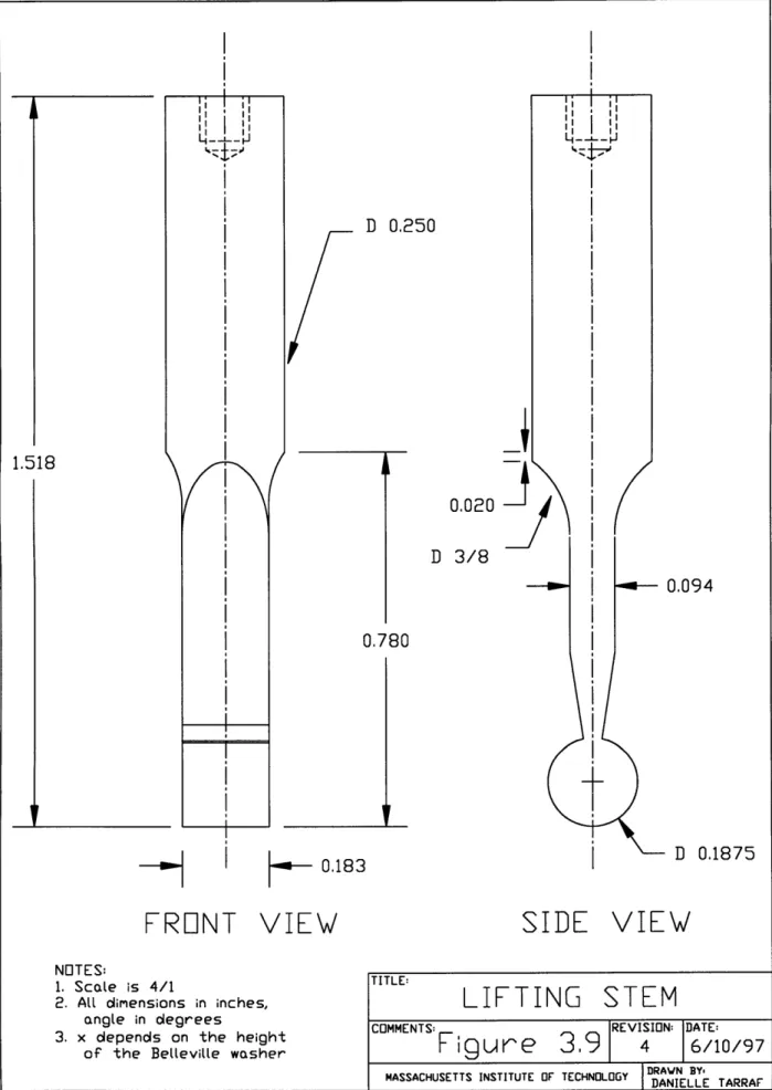
3.4 C over plate... ... . . ... 73 3.5 Cylinder... ... 75 3.6 Piston liner ... ... 77 3.7 M ounting base... 79 3.8 Piston... ... 8 1 3.9 L ifting stem .. ... 83 3.10 Vane m odifications... ... 85
3.11 Com pressor m odifications. ... 87
3.12 Variable Capacity Compressor shown in normal operation mode... 89
3.13 Variable Capacity Compressor shown in unloaded mode... 91
3.15 Sectional view of the compression mechanism and bearings... 93
3.16 Top view of pump and one bearing after addition of sealing cover plate ... 94
4.1 Schematic diagram of the compressor test stand... 97
4.2 Schematic diagram of the compressor test stand after modifications... 104
4.4 Compressor suction and discharge pressure variation over two cycles
(tcycle=105s, R= 1.18)... 112
4.5 Compressor suction and discharge temperature variation over two cycles (tcycle=105s, R=1.18)... 113
4.6 Compressor instantaneous power consumption over two cycles (tcycle=105s, R = 1.18 )... 1 13 4.7 Compressor suction and discharge pressure variation over two cycles (tcycle=59s, R =0.97)... ... 114
4.8 Compressor suction and discharge temperature variation over two cycles (tcycle=59s, R=0.97)... 114
4.9 Compressor instantaneous power consumption over two cycles (tcycle=59s, R = 0 .97 )... 1 15 4.10 Air temperatures at evaporator inlet and outlet (R= 1, tcycle=6 0s) ... 117
4.11 Air temperatures at evaporator inlet and outlet (R= 1, tcycle=40s) ... 117
4.12 Air temperatures at evaporator inlet and outlet (R= 1, tcycle=20s)... 118
4.13 Air temperatures at evaporator inlet and outlet (R= 1, tcycle= 10s) ... 118
4.14 Evaporator and condenser pressures (R=1, tcycle=60s)... 120
4.15 Evaporator and condenser pressures (R=1, tcycle=40s) ... 120
4.16 Evaporator and condenser pressures (R=l, tcycle=20s)... 121
4.17 Evaporator and condenser pressures (R=l, tcycle=10s) ... 121
4.18 Evaporator and condenser pressure variation over 40 seconds for 4 tests: Normal operation; R=1, tcycle=10s; R=l, tcycle=4s; R=0.33, tcycle=8S... 125
4.19 Compressor power consumption for various vane states... 130
4.20 Voltage transient during motor start-up... 133
4.21 Current transient during motor start-up... 133
List of Tables
2.1 Numerical values of geometric parameters of the Carrier EDB240 compressor 27
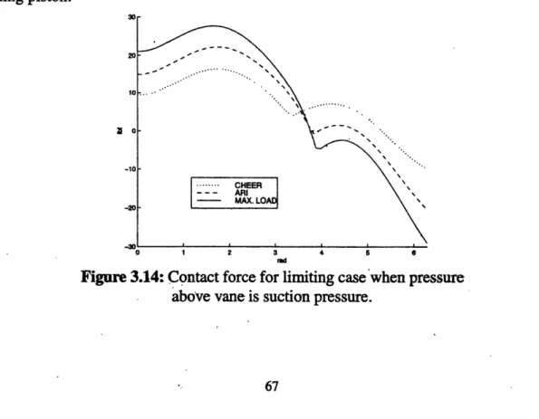
2.2 CHEER, ARI and MAX. LOAD compressor testing conditions... 52
4.1 Pre and post modification test results at ARI conditions... 101
4.2 Modified compressor test results at ARI conditions, modified test stand used.. 105
4.3 Test data for variable capacity tests, 57s/48s and 29s/30s loaded and unloaded cycles... . . 110
4.4 Characteristic cycle parameters for the two tests... 111
4.5 Average evaporator and condenser pressures... 123
4.6 Sum m ary of system perform ance... 126
4.7 Test characteristics... ... 128
Nomenclature
a(t) Acceleration of the vane as a function of time [in./s2]
a(O) Acceleration of the vane as a function of crank angle [in./s2]
Ad(O) Instantaneous projected area of the discharge (compression) volume [in2]
As(0) Instantaneous projected area of the suction volume [in2]
amp Acceleration of the mechanism piston [in/s2]
b Half width of the rectangular area of elastic contact [in.]
B Brinell hardness [psi]
c Radial clearance between pump and compressor housing [in.] Ccycle Average system capacity over one load/unload cycle [BTU/hr] C1 Average system capacity during the loaded phase [BTU/hr]
COP Coefficient of performance [ ]
COPn System COP under normal operation [ ]
Cp Specific heat at constant pressure [BTU/lbm 'F] dch Inner diameter of cylindrical compressor chamber [in.] drp Outer diameter of rolling piston [in.]
e Rolling piston (shaft) eccentricity [in.]
EER [BTU/W hr]
Ei Modulus of elasticity [psi]
er Coefficient of restitution [ ]
f Frequency of rotation of the driving motor shaft [Hz]
F Flowmeter frequency measurement [Hz]
F Maximum contact force due to Hertzian contact [lbf]
FC Contact force exerted by the rolling piston on the curved vane tip [lbf] F, Vane inertia force [lbf]
Fmp Differential pressure force on the mechanism piston [lbf] Fs Spring force acting on the top edge of the vane [lbf]
F1 Force on top edge of the vane due to refrigerant at discharge conditions [lbf]
F2 Resultant pressure force on vane surface facing guide, discharge side [lbf]
F3 Resultant pressure force on vane surface facing guide, suction side [lbf]
F4 Resultant force on flat vane surface exposed to compression chamber [lbf]
F5 Resultant force on flat vane surface exposed to suction chamber [lbf]
F6 Resultant pressure force on curved vane tip in compression chamber [lbf]
F7 Resultant pressure force on curved vane tip in suction chamber [lbf]
G Calibration factor
hch Depth of cylindrical compressor chamber [in.] hn Height of notch in vane [in.]
HRC Rockwell Hardness [ ]
hI Enthalpy of refrigerant at compressor suction [BTU/lbm]
h2,S Enthalpy of refrigerant at compressor discharge, assuming isentropic
compression [BTU/lbm]
h3 Enthalpy of refrigerant at condenser outlet [BTU/lbm]
h4 Enthalpy of refrigerant at evaporator inlet [BTU/lbm]
J 32.2 ft-lbm/lbf-ft2 k Spring constant [lb/in.]
K Calibration factor
KE Kinetic energy [lbf-in]
L Distance between geometric center of rolling piston and center of curvature of vane tip. L=rv+rrp. [in.]
1o Spring free length [in.]
1, Length of vane [in.]
1(0) Instantaneous spring length as a function of crank angle [in.] m Mass flow rate of refrigerant [Ibm/s]
mair Mass flow rate of air across the evaporator [Ibm/s]
mmp Mass of the mechanism piston [Ibm] mv Mass of vane [lb]
n Speed of rotation of the driving motor shaft [rpm]
P Pressure [psi]
Pavg,c Average compressor power consumption [kWatt] Pavg, Average system power consumption [kWatt] system
PC Condenser pressure [psig]
Pcycle Average compressor power consumption over one load/unload cycle [kWatt] Pd Discharge pressure [psig]
Pe Evaporator pressure [psig]
P, Fluid pressure at flowmeter (de-superheater loop experiments) [psig]
Pin Power input to compressor [kWatt]
P, Average compressor power consumption during loaded phase [kWatt] Ps Suction pressure [psig]
Pstart Average compressor power consumption during motor start-up [kWatt] Pu, PU Average compressor power consumption during unloaded phase [kWatt] P(6) Instantaneous pressure in compression chamber as a function of crank angle
[psig]
q Maximum Hertzian contact pressure [psi]
Qcoo
1 Cooling load of the system (cooling rate) [BTU/hr]rch Inner radius of cylindrical compressor chamber [in.] rrp Outer radius of rolling piston [in.]
rv Radius of vane tip [in.]
s Vane stroke [in.]
S Motor slip (%) [ ]
t Time [s]
tcycle Cycle time (ton+toff) [s]
ton Time duration of loaded phase [s] toff Time duration of unloaded phase [s]
toff, Critical time duration of the unloaded phase beyond which it is energy effi-critical cient to shut motor off [s]
tp Thickness of pump wall [in.] t, Thickness of vane [in.]
U Internal strain energy [lbf-in.]
V Volume [in3]
v(t) Velocity of the vane as a function of time [in./s]
v(O) Velocity of the vane as a function of crank angle [in./s] VD Displacement volume [in3]
Vms Volume of the mechanism lifting stem [in3]
Vrp Velocity of the rolling piston along the line of impact [in./s] vv Velocity of the vane along the line of impact [in./s]
Vv Volume of the vane [in3]
Vv/rp Vane velocity relative to the rolling piston along the line of impact [in./s] wn Average width of notch in vane [in.]
wv Width of vane [in.]
x(0) Displacement of the vane as a function of crank angle [in.] x,y; Rectangular coordinates
X,Y
0 Crank angle of the rolling piston (0=0 <=> Top dead center) [rad]
o0 Angular speed of rotation of the rolling piston center about the center of the compression chamber. o=dO/dt. [rad/s]
(O0n Natural Frequency of the vane/lifting stem/spring system [Hz] 8 Maximum deflection due to Hertzian contact [in.]
AP Pressure difference between the evaporator and condenser (Pc-Pe) [psig]
P, Polar coordinates
00 Crank angle at which a sealed compression chamber forms [rad]
y Specific heat ratio (Cp/Cv) [ ]
i1 Motor efficiency [ ]
Yu Ultimate tensile strength [psi]
Imax Maximum allowable shear stress [psi]
1)i Poisson's ratio [ ]
p Dynamic viscosity of refrigerant [micro poise] P Density of refrigerant [lbm/ft3]
ATair, Average temperature difference of air across the evaporator [oF] evap
Connecting rod angle [rad]
%Cap Percentage of normal operation capacity
Subscripts
ch Cylindrical compressor chamber
d Discharge
i Initial
f Final
n Vane notch
p Pump
rev Reversible process
rp Rolling Piston
s Suction
test Actual testing conditions
v Vane
1 State at compressor suction
2 State at compressor discharge
3 State at condenser outlet
Chapter 1
Introduction
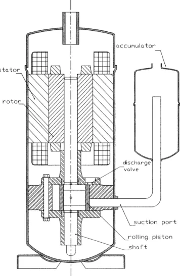
The compressor examined in this study is the rolling piston type rotary compressor. The typical construction features of a hermetic type rotary compressor are shown in Figure 1.1.
Figure 1.1: Typical construction features of a hermetic rolling piston type rotary compressor
1.1 Basic Operation of a Rotary Compressor
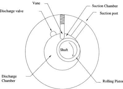
Some familiarity with the basic operation of this type of compressor is essential to the understanding of the work presented in this thesis. A simple schematic of the compression device in a rolling piston type rotary compressor is shown in Figure 1.2.
Suction Chamber
Discharge valve Suction port
Discharge
Chamber Rolling Piston
Figure 1.2: Schematic of the compression mechanism in a rolling piston type rotary compressor
The major components of the compression mechanism are: the cylindrical chamber, which includes the suction and discharge chambers. Within this chamber are the rolling piston, the eccentric shaft, and the reciprocating vane. The chamber is in contact with refrigerant at suction and discharge conditions via the inlet (suction) port and the pressure activated discharge valve, respectively.
The shaft is driven by the motor and rotates eccentrically about the center of the cylindri-cal chamber. The rolling piston rotates eccentricylindri-cally with the shaft. It also slides relative to the shaft, thus rotating about its axis. As it rolls, the rolling piston contacts the wall of the cylindrical chamber thus forming a sealing point. During normal operation, the vane is mainly pressure loaded by the fluid at discharge pressure which acts on its top surface. It pushes against the rolling piston. Hence, a second sealing point is maintained under nor-mal operation. The position of the rolling piston as the system goes through one complete revolution of the shaft is illustrated in Figure 1.3. The suction chamber (s) is always in contact with fluid at suction pressure via the inlet port. As soon as the piston / chamber wall sealing point crosses the inlet port, a closed discharge chamber (d) is formed. Fluid at suction conditions is trapped within it. Further rotation of the piston causes this discharge chamber to decrease in volume continuously, thus building up fluid pressure in the cham-ber. Once the chamber pressure exceeds the compressor discharge pressure, the pressure unbalance activates the discharge valve causing it to open, thus discharging the high
pres-sure fluid. When the piston reaches top dead center of its travel, the two sealing points merge into one. A single chamber exists at this instant, and the cycle repeats itself. The spring shown in Figure 1.2 is important during system start-up. That is, before the pressure on the discharge side builds up sufficiently to hold the vane down against the rolling pis-ton. During normal operation, it contributes only mildly to the force acting on the top side of the vane, as will be shown in a later chapter.
Figure 1.3: A complete compression cycle undergone by a rolling piston type rotary compressor.
1.2 The Need for Variable Capacity
Rolling piston type rotary compressors have a number of advantages, namely: High effi-ciency and reliability, low noise, relatively light weight and small size compared to other compressors having the same capacity [1]. Thus, this type of compressor is widely used in domestic air-conditioning and refrigeration units. Constantly changing environmental con-ditions impose varying loads and operating concon-ditions on the system. Hence the need for variable capacity operation, to ensure the comfort of the user and especially as the require-ments of energy saving and conservation of resources grow more stringent.
1.3 Variable Capacity: Typical Methods
Vapor compression systems are the most commonly employed systems in domestic refrig-eration and air-conditioning applications. Variable capacity is generally achieved in these systems by varying the mass flow rate of refrigerant in the system. This, in turn, requires varying the average mass flow rate of fluid through the compressor driving the system. Typically, that is done by using a variable speed drive for the pump. As a result, the speed of rotation of the eccentric rolling piston changes. Hence, the frequency at which the com-pressor releases a charge of high pressure fluid changes, and thus the average mass flow rate of the fluid changes as well. Usually, some electronics are used to excite the motor driving the pump at various frequencies. The cost of the electronics can be quite high, at
least of the order of $100/kW. This contributes considerably to the initial cost of the sys-tem.
1.4 Variable Capacity: The New Concept
It seems advantageous to devise a method for varying the capacity of rolling piston type rotary compressors without having to resort to variable speed motors. This would elimi-nate the need for high cost electronics. In turn, that would lower the initial cost of the sys-tem. Obviously, the advantage is only real provided the new technique provides comparable performance during operation. Otherwise, the savings in initial costs would be lost in operating costs over the life of the compressor. This study attempts to explore and develop a new concept for varying compressor capacity. The new technique should per-form as efficiently as the typical variable speed motor method used in order to be truly competitive.
Looking at reciprocating positive displacement compressors for ideas; The most common method for varying compressor capacity is by holding the suction valve open for a certain number of cycles. When the suction valve is open, the fluid in the compressor remains in contact with the suction side. Hence, as the piston travels, the fluid is pushed in and out of the compression space, without ever reaching a high enough pressure to activate the dis-charge valve. This decreases the average mass flow rate of refrigerant through the com-pressor, thus decreasing its capacity. By controlling the number of cycles during which the suction valve is held open and those in which it is closed, the capacity of the system can be controlled. If a similar idea were to be implemented to the rotary compressor at hand, the first obvious problem is that no suction valve exists. Instead, a suction (or inlet) port is used, and this connects the suction volume to fluid at suction conditions at all times. Fur-ther examination of the situation reveals that in a reciprocating compressor:
i. The suction chamber and the discharge chamber are identical.
ii. Holding the suction valve open opens up the otherwise sealed compression (discharge) chamber to suction. Hence, the upwards piston motion can no longer sufficiently pressur-ize the now large mass of fluid to a pressure higher than discharge.
Based on the above, two scenarios come to mind for the rotary compressor. The first is the addition of a suction valve, which would be kept open all through normal operation, and which will be closed intermittently during lower capacity operation. As a result, after an "initial" lost cycle, the discharge volume can no longer be replenished with fresh refriger-ant at suction conditions. Hence, the volume ratio characteristic of the compressor will no longer suffice to raise the pressure of the small amount of remaining refrigerant. The other scenario consists of lifting the vane for some number of cycles, thus breaking the dis-charge chamber's seal. As a result, as the piston rotates, the fluid is in contact with suction and is just moved around in a space that is invariant in volume. Hence, its pressure does not rise significantly and the discharge valve remains closed during this time.
Although the above two scenarios are quite different in concept and implementation, they both achieve the same end result: varying the average mass flow rate of fluid through the compressor. A colleague, Dr. Greg Nellis [2], carried out a preliminary analysis to com-pare the relative advantages of the two methods. The results seemed quite decisive: Sce-nario two, the Vane Lifting Technique, seemed clearly superior in terms of higher efficiency, as reflected by the EER value. This conclusion holds assuming that:
i. The vane lifting mechanism can be properly controlled, that is, activated and deactivated at the optimum piston position.
ii. The vane lifting mechanism could operate at the required speed (achieve full reversal in -16.6 milliseconds, equivalent to the time required by the piston to undergo a complete revolution if motor slip is 0).
1.5 Overview of this Study
The purpose of this investigation is twofold. First, to investigate the feasibility of design-ing and constructdesign-ing a satisfactory vane liftdesign-ing mechanism. Second, to assess the technical soundness of the new concept. Stated simply, it aims at answering the following two ques-tions: Can this idea be implemented to really achieve variable capacity? Can a suitable mechanism be devised and constructed?
The approach taken is largely practical and experimental. Analysis and modeling are kept to a strict minimum given the limits imposed by time constraints for the project.
In the next chapter, a simple model is developed to study the kinematics and dynamics of the vane motion. The interaction between the vane and the rolling piston is also studied and the resulting stresses are calculated. Finally, given the possibility of impact between the vane and the rolling piston, such a situation is modeled and analyzed. The resulting impact stresses are determined and the possibility of failure is evaluated.
Chapter 3 follows the evolution of the design from a concept to its final form. It includes detailed working drawings of the various components of the mechanism, as well as an assembly drawing. It also contains a description of the modifications made to the existing compressor to fit and mount the mechanism. The construction of a prototype mechanism is described in this chapter as well.
A series of tests were done on the modified compressor. These ranged from simple tests on a compressor test stand to testing the operation of the compressor in an actual system. This is the subject of Chapter 4. The experimental apparatus and test conditions are described, the test data is presented and then analyzed for the various tests.
The final chapter wraps up the topic: Based on the test results, the concept is evaluated, and so is the actual mechanism design. Recommendations are made for further work.
Chapter 2
Analysis
2.1 Motivation for the Analysis
As the name indicates, the vane lifting mechanism's function is to lift the vane. The mech-anism should be able to provide enough force for that purpose. Also, it should be able to lift the vane fast enough so that it doesn't interfere with the motion of the rolling piston. To translate "enough force" and "fast enough" into quantitative terms, a knowledge of the dynamics and kinematics of the vane motion is required. Once the above are determined, another important question arises: How critical is proper timing to the success of the vane lifting mechanism? In other words, can we tolerate having the mechanism let go of the vane when the crank angle1 is non zero? Answering that involves modeling of the result-ing impact, determinresult-ing the correspondresult-ing impact stresses, and evaluatresult-ing their effect on the system components.
The motivation for this part of the thesis is to seek answers for all the above questions. This chapter contains a kinematic analysis, a dynamic analysis, a stress analysis and an impact analysis of the vane and rolling piston. The models used for the analysis are described in the coming sections. The simplifying assumptions are stated. The relevant equations are derived and then implemented. Although the theory and models hold for any size rolling piston type rotary compressor, the numerical values of various parameters, and consequently the dimensions of the mechanism depend on the size of the compressor. In this work, the focus is on the Carrier EDB240 rolling piston type rotary compressor. The numerical values of all parameters and the results given pertain to this particular compres-sor. Thus, section 2.2 overviews the main construction features and the relevant dimen-sions of the compression device in the EDB240 compressor.
A note on units: In spite of the author's preference for SI Units, the bulk of the work is done in US Customary Units. The equivalent SI measurements are provided in certain instances. That is due to the apparent preference of advisors and collaborators on this project for English units.
2.2 The Carrier EDB240 Compressor
The Carrier EDB240 is a rolling piston type rotary compressor; It is used in domestic vapor compression air-conditioning systems of 24,000 BTU/hr capacity (2 Tons of refrig-eration). The working fluid is Freon (Refrigerant R-22).
Figure 2.1: Graphic explanation of compression chamber and rolling piston dimensions
Figure 2.1 illustrates the nomenclature for the relevant geometry of the compression chamber and the rolling piston. dch is the diameter of the cylindrical compression cham-ber, and drp is the outside diameter of the rolling piston. rch and rrp are the corresponding radii. The rolling piston is a hollow cylinder that mounts on a shaft. This detail is not shown in the figure because it is irrelevant in this context. e is the eccentricity of the shaft, and hence the rolling piston, to the axis of the compression chamber. hch is not shown in the figure. It represents the height of the compression chamber (perpendicular to the page). 0 is the crank angle of the rolling piston: 0=0 corresponds to the piston being at top dead center. tp is the thickness of the pump wall in the vicinity of the vane (the thickness varies slightly at some other locations due to minor details).
Figure 2.2 shows the vane and the nomenclature of the relevant vane dimensions. The fig-ure is self explanatory. The notch on the top edge of the vane seats the loading spring. Note that wn represents the average width (the notch is tapered). The relevant dimensions
of the spring are its original length, 10, and its minimum length, Imin. The spring constant is
denoted by k.
A note about materials: The vane is made of M2 tool steel, through hardened to Rockwell hardness 60C - 65 C. The rolling piston is made of gray cast iron, through hardened to 45C -55C.
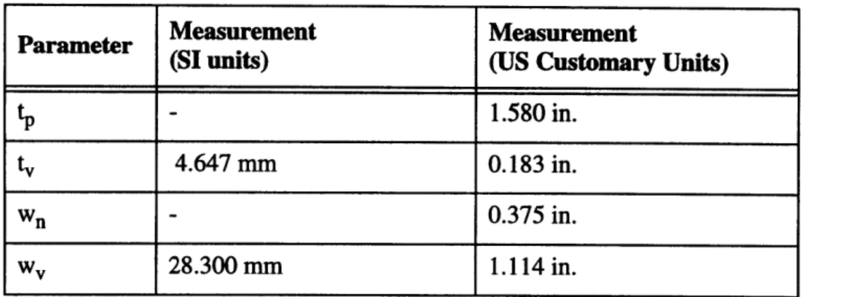
The numerical values of all relevant dimensions are listed for convenient reference in Table 2.1 below. The compressor was designed using metric units, hence the values of some parameters are taken off company production drawings in millimeters and then con-verted to inches for use in this work.
Table 2.1: Numerical values of geometric parameters of the Carrier EDB240 compressor
Measurement Measurement
Parameter
(SI units) (US Customary Units)
dch 59.004 mm 2.323 in. dp 48.889 mm 1.925 in. e 5.048 mm 0.199 in. hch 38.993 mm 1.535 in. hn - 0.119 in. k - 8.29 lb/in. 10 36.000 mm 1.417 in. Imin - 0.56 in. 1, 38.976 mm 1.534 in. m- 0.083 lb rch - 1.162 in. r- 0.963 in. rv 4.500 mm 0. 177 in.
2.3 Kinematic Analysis
2.3.1 Model and Equations
The motion of the vane is analyzed in this section. Equations for the displacement, veloc-ity and acceleration of the vane are developed, both as functions of crank angle and of time (with a suitably defined time origin). The analysis is purely geometric, based on the assumption that the vane remains in contact with the rolling piston at all time. This assumption is necessarily true if there is no leakage. The only exception is during the first few cycles after initial start-up, when the vane may bounce on the rolling piston.
Figure 2.3: Contact geometry between vane and rolling piston
A simple two-dimensional diagram of the contact geometry between the vane and the roll-ing piston is presented in Figure 2.3. O is the geometric center of the cylindrical
compres-Measurement Measurement
Parameter
(SI units) (US Customary Units)
tp - 1.580 in.
tv 4.647 mm 0.183 in.
wn - 0.375 in.
sion chamber. C is the center of the rolling piston, and C' is the center of curvature of the vane tip. Define a coordinate axis, x, which tracks point C' as the vane moves. The origin of this axis, 0', corresponds to the location of point C' when the vane is at top dead center of its travel. Thus, x represents the displacement of the vane from top dead center. A is the point of contact of the rolling piston and vane. A travels back and forth along the vane tip. The crank angle 0, defined in the previous section, is the clockwise angle that OC makes with OC'. Let
4
be the angle between C'O and C'C.4
will be referred to as the connecting rod angle, for reasons that will become clear as we proceed. The eccentricity, e, is shown, as well as a new parameter L. L is the distance between C' and C. A simplifying assump-tion is made: no deformaassump-tion occurs at either vane or rolling piston surfaces. That is, the contact remains a line contact, and hence distance L is constant, equal to the sum of the radii of curvature of the two contacting surfaces.The rolling piston is driven by the motor shaft. The shaft is cylindrical and rotates off-cen-ter. The axis of rotation of the shaft is parallel to its axis of symmetry and passes through point O. Hence, point C follows a circular path centered at O. The rolling piston may also slide circumferentially around the shaft. The motion is a rotation about C, and hence does not affect the location of this point. Therefore, this motion will not be considered in the analysis because it is irrelevant.
C
L --- -- e
O' x
Figure 2.4: Kinematic model of vane and rolling piston as a Slider Crank mechanism.
Assume that the rolling piston orbits in the clockwise sense in Figure 2.3. The system con-sisting of the vane and the rolling piston can be modeled as a Slider Crank mechanism, as shown in Figure 2.4. C'C and OC are analogous to the connecting rod and the crank, respectively, of a slider crank mechanism. Hence, the names of the corresponding angles, 0 and 0. Distance 00' (00') is fixed. When the vane is at top dead center, both angles 0 and 0 are 0. Hence;
O' = e+L (2.1)
When the vane is at any other position,
Equating the right hand sides of equations 2.1 and 2.2 and rearranging, we get:
x = e(1 -cos0) + L(1 -coso) (2.3)
Sine Law applied to triangle OCC' gives:
e
sin = sin (2.4)
L (2.4)
Hence:
cosO = 1-(sino)2 = 1-sin0f (2.5)
Replacing the value of coso from equation 2.5 in equation 2.3, we get an expression for vane travel from top dead center as a function of crank angle.
2L 22(2.6)
X(o) = e+ L-ecos- L- (esinO)2 (2.6)
The velocity and acceleration of the vane as a function of crank angle are the first and sec-ond time derivative, respectively, of the above expression. Using the chain rule of differen-tiation: dx(0) dx(o) dO () dt dO dt (2.7) d 2x () d dx() d- d 2X() (dO 2 d20 dx(°) (2.8) a 2= - 7 dt (2.8) dt2 dtd t d 2 dt2 dO
dO/dt is the angular speed of rotation (o) of point C about point O. o is set by the rota-tional speed of the motor shaft, and is constant for a constant speed drive (which is the
d2 do
case for the EDB240 compressor). Thus, d-2 -= 0, and the second part of the right
dt dt
hand expression in equation 2.8 goes to zero. Equations 2.7 and 2.8 reduce to:
dx
(e) = O" d- (2.9)
d2
Carrying out the differentiations, we get the expressions for vane speed and acceleration as a function of the crank angle of the rolling piston:
2
e c. sin26
() = e- sin + sin2(2.11)
22 4 2 2 2 em 0 cos20 em * (sin20) a() = e0 -cos 0+ + (2.12) J L2_ (esin0)2 4[L2-(esin0)2] 3/ 2 dO
Starting from the definition of o = .Integrate to get an equation for the crank angle as dt
a function of time:
0t)= =(t) JOdt+ dt +Oo00 (2.13)
Taking the origin of the time axis to be when the vane is at top dead center. From geome-try, the corresponding angle 0, 00, is zero. Replacing 0 by cot in equations 2.6, 2.11 and 2.12. We get expressions for the displacement, velocity and acceleration of the vane as a function of time.
X(t) = e + L - e cosot - L2 -(e - sinot)2
(2.14)
2 2
v(t) = e- sint + 2L2 -(e sinot)2 (2.15)
2 2 4 2 2
2 e 0 - cos2cot e 0- (sin2ot)
a = e) * cos t + + (2.16)
(tL2 -(e ) sinwt)
2 4[L -(e sin0t)2]3/2
Finally, the stroke of the vane, s, is by definition the total distance covered by the vane as it travels between top and bottom dead centers. When the vane is at bottom dead center, the distance 00' is:
O O'=(L-e)+s (2.17)
Equating the right hand sides of equations 2.1 and 2.17, we get that the stroke s = 2e. Let the frequency of rotation of the motor shaft be f. The corresponding angular speed of rotation of the rolling piston about center O is:
o = 2 tf (2.18)
2.3.2 Numerical Simulation
The Carrier EDB240 compressor is driven by a single phase induction motor. If motor slip is zero, it drives the shaft at a rotational speed n=3600 rpm. In practice, motor slip (S) at full load is around 1.5%. Due to this, the rotational speed of the motor drops to about 3546 rpm.
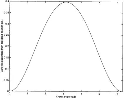
For the purpose of the simulation, the assumption is that S=O. Hence, n=3600 rpm equiva-lent to a frequency of rotation f of 60 Hz. Thus, (o=377 rad/s. The equations of motion were plotted versus crank angle using Matlab. The resulting graphs are shown in Figures
2.5, 2.6 and 2.7. 04 035 03 V0 25 E 0.2 S015 -5 .1 0 05 0 0 1 2 3 4 5 6
Crank angle (rad)
Figure 2.5: Vane displacement from top dead center as a function of crank angle
80 60 40 20 0o (D
/O
> 0 1 2 3 4 5 6 Crank angle (rad)0-a -1 - -2--3 1 I 0 1 2 3 4 5 6
Crank angle (rad)
Figure 2.7: Vane acceleration as a function of crank angle
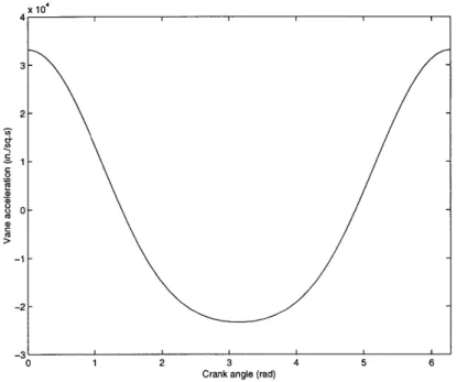
The maximum displacement is found to be 0.398 in., as expected (twice the eccentricity). Negative velocity corresponds to the vane being in the upwards stroke, moving towards top dead center. Negative acceleration signifies either a decceleration (between 0--=/2 and 0---)or an acceleration in the negative x direction (between 0---n and 0=3t/2).
The maximum speed at which the vane moves is found to be 76.16 in./s. The maximum acceleration/decceleration the vane encounters during its travel is 33,250 in./s2
2.4 Dynamic Analysis
This section presents a very simple dynamic model of the vane. The forces considered in the analysis are the spring force and the various contact and pressure forces. Frictional effects are completely neglected. The assumption is that all moving surfaces are ade-quately lubricated. (Namely the contact surface between the vane tip and the rolling pis-ton, and the sliding surface between the faces of the vane and the vane guide). Hence, the resulting friction coefficients should be small and the corresponding frictional forces min-imal in effect.
2.4.1 Model and Equations
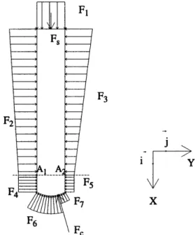
A free body diagram of the vane (neglecting friction) is shown in Figure 2.8. Fs is the
the top edge of the vane. Fe is the contact force exerted by the rolling piston on the curved
vane tip at the line of contact. The direction and point of application of Fe vary
continu-ously throughout a cycle. F5 is the resultant load on the flat section of the vane surface
exposed to refrigerant in the suction chamber. F4 is the resultant load on the flat surface
due to refrigerant in the compression chamber. The pressure in this chamber cyclically varies between suction and discharge. The corresponding resultant forces on the curved vane tip due to contact with fluid at same conditions are F7 and F6 respectively. The
pres-sure distribution of the fluid within the small clearance space between the vane and its guide on either side of the vane is assumed to be linear. The resultant pressure forces are denoted by F2 and F3 as shown. The inertia force is not shown in Figure 2.8 but will be
considered in the analysis of course.
F 1
F7 X
F 6 F3
Figure 2.8: Free body diagram of the vane neglecting friction
Call the point of contact between the vane and the rolling piston point A. Consider an imaginary line that connects the edges of the vane guides. Let the intersection of this imaginary line with the vane be points A1 and A2 on the discharge and suction sides,
respectively. The location of these three points varies with crank angle.
The moments caused by all the forces about points A1 and A2 need to be determined. The
sign convention adopted is that clockwise moments and counterclockwise moments are considered positive about points A1 and A2 respectively. The purpose of these moment
calculations and the choice of sign convention is not immediately obvious, and will be explained in detail in the following section.
Spring Force
The spring rests in the vane notch and pushes against the compressor housing. The clear-ance c between the outer edge of the pump and the housing is very small, of the order of a few thousands of an inch. Hence, it will be neglected.
w
h11
1(6)l0
1
c
hn
V
At top dead center At distance x from
top dead center Figure 2.9: Geometry relevant to spring force analysis
When the vane is at top dead center, from geometry as shown in Figure 2.9:
tp = 1(o) + WV - hn (2.19)
1(0) denotes the length of the spring when the vane is at top dead center. When the vane moves a distance x from top dead center, the spring correspondingly elongates by the same distance x.
tP = l( ) + (WV - x(O) - hn (2.20)
Hence, the instantaneous spring length as a function of crank angle is:
1(o) = t, + hn-w v + x(o) (2.21)
The resulting instantaneous spring force is:
Fs(o) = k Ale) = k -(lo - ()) (2.22)
Replacing equation 2.6 for x(() in equation 2.21 and then equation 2.21 for 1(0) in equation
2.22, we get an expression for the magnitude of the spring force on the vane as a function of crank angle.
Fs(o) = k. [lo-t,-h n + wv-e-L + ecos+ L2- (esin) 2 (2.23)
The spring is always in compression. Hence, the resulting spring force can be represented vectorially as:
- >. (2.24)
Fs(o) = F(o). i
cases (due to the sign convention adopted). It is given by:
tv (2.25)
MS, A(O) = MS,A2() = FS(). (2.25)
Pressure Forces
The vane is in contact with fluid at all points on its surface except for points along the line of contact with the rolling piston. Boundary lubrication at that location allows for some metal to metal contact. Hence, the vane is subjected to pressure forces on all its surfaces. The pressure forces acting on its sides are not shown in Figure 2.8 (If they were, they would be perpendicular to the plane of the diagram). The reason being that they should be equal and opposite due to similar conditions, and thus would balance out. All other pres-sure distributions acting on the vane surfaces are shown in Figure 2.8. The task undertaken in this section is to reduce these pressure distributions into equivalent point forces, denoted by Fi, i going from 1 to 7, with suitably determined points of application. The resulting pressure force diagram is shown in Figure 2.10
F1
F3
F2
F4 F5
F6 F7
Figure 2.10: Equivalent pressure forces
Force F1 is the resultant of a uniformly distributed load on the top edge of the vane. Hence,
it acts at the midpoint of the edge (It has the same point of application as the spring force). In magnitude, it is equal to the product of the fluid pressure and the area subjected to it. Hence:
- (2.26)
F1 = Pd.(lv.tv).i
The moment caused by this force about both points Al and A2 is always positive and is given by:
1 2 (2.27)
Determining equivalent forces F2 through F5 is a little bit trickier. That is mainly because
the area upon which a given fluid pressure profile acts is a function of vane position with respect to its guide.
Figure 2.11: Vane dimensions relevant to the pressure distributions on vane face
Forces F2 and F3 are due to a linear distribution of pressure acting on an area Aa(O)=la(O).lv.
Forces F4 and F5 are due to a uniform pressure distribution acting on area Ab(o)=lb(0).lv. In
Figure 2.11, the dotted straight line connects the two edges of the vane guide. Note that the clearance co between the vane and its guide is highly exaggerated in this diagram. Also, it
is shown to be symmetric, which is generally not the case. Ob denotes the midpoint of this straight line. Oa is the midpoint of the dotted arc shown. This arc is the extension of the
pump chamber wall circular profile. Thus, Oa also coincides with the location of the vane
tip when the vane is at top dead center. In the analysis that follows, points Oa and Ob are assumed to coincide. This assumption should not introduce much error given that the vane thickness is much smaller than the radius of the cylindrical chamber. That is,
tv<<rch-Figure 2.12: Vane tip geometry
Now refer to Figure 2.12 for a closer look at the vane tip geometry. Pythagora's Law gives that:
-I~--2 =v(+2 (2.28)
S2
Hence, 2 =t 2 (2.29) and angle : = asin-tv (2.30) .2rv)From Figure 2.11, it is obvious that, with the assumption made regarding Oa and Ob:
lb(o) = x(o) - Z;(x(o) 2 z) and = 0;(x(0) <z) (2.31)
wv = la(O) + lb() + Z = la(O) = wv - Z - lb() (2.32)
Replacing for x(O) and z from equations 2.6 and 2.29 respectively, we get that:
o)ILr+r2 2 (2.33)
lb(O) = e + L - r+ r-ecosO- L2-(esinO) 2;0
X(o) z;x(o) < z
1 2 _ 2 (2.34)
la(o) = - e - L + ecos0 + L2 - (esinO)2 (2.34) Thus, equivalent pressure force F5 acts at a distance 1/2 lb(0) from point A2 (defined
ear-lier) and is given by:
4 > (2.35)
Fs(0) = -Ps - (b(o) I )" J
Its moment about points A1 and A2 is the same in magnitude, but varies from positive to
negative respectively for the sign convention defined earlier:
- - 1 2
M5, A,(o) = M5,A2() P 1 b(O) (2.36)
Following similar reasoning:
F4(o) = P(o) v . lb(0)
(2.37)
P(0) is the pressure in the compression chamber. As mentioned previously, it varies during
each cycle from suction to discharge pressure. The compression process is modeled, and an expression for P() is determined later in section 2.4.2.
The pressure distribution on either face of the vane within the vane guide is assumed to be linear. On the discharge side, it varies from Pd to P(0) over a length la(e). On the suction side, it varies from Pd to Ps over the same length.
To avoid going over the same derivation twice, consider in general a linear pressure distri-bution acting on an area of length A and of unit width, as shown in Figure 2.13. f is a vari-able that represents distance from the origin O. Let the pressure at f=O be Pi and at f=A be Pf.
Figure 2.13: A
A f
linear pressure distribution.
The effect of this pressure distribution can be modeled by one equivalent force, F, applied at a specific distance 8 to be determined. The pressure distribution can be expressed math-ematically as:
P(fP
f
+ PiP(f)= A f+P 2i
The equivalent force per unit width is the infinitesimal sum of the elements of force acting on infinitesimally small areas.
F = JP(f)df = Jfdf+Pi df =
1
..F = 2 (Pf + Pi) A
(PPi) + PiA
(2.40)
This force should be applied at a distance 8 from point O such that the moment caused by the linear pressure distribution and that by the equivalent force about point O are equal.
M = P(f)fdf = F8 (2.41) Thus, P f - Pi A
J
fdf+Pif Afdf = F8 - 3 + PA2 = 2(Pf + Pi)A8 S= (2P f + P) A (2.42) 3(p f + pi)Applying the results given by equations 2.40 and 2.42 to determine forces F2(6) and F3(0) is simple. The corresponding variables Pi, Pf and A have to be identified and substituted for in each case. Let f=0 to correspond to the top edge of the vane. Pd corresponds to Pi and la(o) to A for both pressure distributions. For the discharge side pressure distribution, P(O) corresponds to Pi while for the suction side pressure distribution, Ps corresponds to Pi. Substituting in the relevant equations, and keeping in mind that the equations were derived per unit width, we get:
S 1 (2.43)
F2(o) = 21V(P(o) + Pd)la(O) ( 4
4 1 > (2.44) F3(0) = - 1,(P s + Pd)1a(o) " ( (2P(e0) + Pd) '2(0) - 3(P(0) + d) la(O) (2.45) (2Ps + Pd) 3(0) - 3(P + Pd) a() (2.46)
The moments caused by these forces about A1 and A2 are:
M2, A,(0) = -M2, A2(0) = l(P() +Pd)'a(0)[1a(0) - 2(0)]
1 2 P() + 2Pd
-2= 1(P(e)+ Pd)1 a() 3(p + Pd)
M3, A(0) M3,A2(0) = (2.48)
1 -2--- 2
l ,(P +2Pd)[ -e-L+ecos0+ 2 - (esinO)2
The forces due to pressure on the curved edge of the vane, F6 and F7, can be determined
by integrating the elemental pressure forces along the curved surface. The integration is done vectorially, to take into account that the direction of the infinitesimal force at any point changes so as to remain perpendicular to the surface. For that purpose, consider an infinitesimally thin surface strip that extends along the length of the vane and of width ds as shown in Figure 2.14. Define angle y to be the counterclockwise angle that the perpen-dicular h to this area makes with the line of symmetry of the vane through point O'.
Figure 2.14: Schematic of integration along curved vane tip
The area of this strip, represented vectorially in terms of the inwards normal to the surface at that location, is:
dA = Iv, dsn (y)
= I, ds[-cosy -i- siny j]
Correspondingly, the infinitesimal force due to pressure on that strip is:
dF = PdA-)
dF(y) = P -dA(y)
(2.49)
(2.50) Thus, keeping in mind that ds=rv.d0, the total pressure force along a section of the vane tip extending from y-o to "-Yf is:
F = (P. dA(y)) = PI, [-cosy i - siny-
j]rvdy
Yo
P
= Plvr,[siny- sinyf] + Plvr[cosyf-cosyo]i (2.51)Equation 2.51 can be used to determine forces F6 and F7, by substituting the proper values
for y. and yf. Adhering to the sign convention for . on the discharge side, y0=-4 and yf=4 . On the suction side, y0=0 and yf=i. Hence,
F6 = -P()lr,(sine + sino)i + P(o)Ivrv(cos - cosQ)j
F6(0)
=-P(0)v
v[rv + Lvsin i+(o)vv Plr 1- (sin6 )2 - 1-(
2)
(2.52)F7 = Pslvr,(sin4 - sinQ)i + PsIVr(cosQ - cos )j
F7(e) = Pslr[ sin - + Pslvrv 1 - rsin - 1 - (2.53)
Both forces F6 and F7 cause a non-zero moment about pivot points A1 and A2. The
moment arms are hard to calculate explicitly as a function of the crank angle because of the complicated geometry. The point of application of force F6 is along the curved edge of
the vane, at an angle of +j", due to symmetry. Similarly, F7 acts along the edge of the
vane at an angle of -Q, as shown in Figure 2.15.
FA O A2
\
F6
Consider first force F6. It can be decomposed into two components along the coordinate axis defined, F6x and F6y. The moment arm of F6y about points A1 and A2 is the same,
given by: lb() + rvCOS( 2 ) - = X0) + rVcos( 2
-
1]. The moment arm of+
t
s
Hence, the
F6x about A1 is: -rvsin and about A2 is: + r Hence, the
moment of F6 about points A1 and A2 is given by:
rv e" rv
A6, A P(O)lvrv -V + sinO L2 - r vin 2
P)1 rv[ 1 - (jsin 2 - () + rv[cos
-M6, A2 = -P(o) vrv + in [ + r sin +
P)1 rv 1 - (Lsin) - 2 ,v (+ rvCOS(4 - 1]}
0)[
( 1 - - + rv 2.
M6, A,= -P(O)lvrv{- + -sinO] - - rvsin +
1
- L2sin02 2() vCOS-1 (2.54)
1 - (jsin 2 - - v)2] x()+ rv[COS~ - 1 (2.55)
No effort will be made to analytically reduce the above equations to explicit functions of the crank angle 6. The variation of with 0 will be simulated numerically and used in the equations in the next section.
Following a similar procedure, the moment of force F7 can be calculated about points A1
A7
Al sivrv{ - sino - + r sin
]
M7, A = Pslvr SL sine - 2rVL2 l -1 r sin + 2
+ 1
-(
2 1 sin e 2(x(0) + rvcos( 1 (2.57)Inertia Force
The inertia of the vane may be represented as a force acting in the direction opposite to the acceleration of the vane, according to D'Alembert's principle. Thus,
4 m >. (2.58)
FI() = -- A(2.58)
J is required as a conversion factor in this equation because English units are used. J = 3 2.2ft bm = 386.4 in 2 .bm2
lbf . s bf .s2
The moment of the inertia force is either positive about both pivot points A1 and A2 or
negative about both, depending on whether the vane is accelerating or deccelerating. It is given by:
A tv (2.59)
MI, A( ) = MI, A2( ) = --- A( )
Contact Force
Let the magnitude of the contact force as a function of crank angle be Fc(e). An expression for FC(e) cannot be written at this stage: The contact force varies such as to keep the forces acting on the vane balanced along the direction of motion as the vane moves. Based on the assumption of perfect line contact between the vane and rolling piston, the direction of the contact force is necessarily along the line of centers CC'. (Keep in mind that the friction forces are neglected).
The components of the contact force along the X and Y directions are, respectively:
Fc, y(e) = -Fc(e) sin (2.61)
O C Fc(0),x
Figure 2.16: Contact force and geometry
Replacing coso and sino by their values from equations 2.5 and 2.4 respectively, we get the expression for the contact force:
FC(o) = F, x(e) i + Fc, y(e)' J o) -F(2.62)
C(= -Fc(e) cos i -FC(O) sing j
tv/2 r sinV
A
1 O' A2 b lb) rvcoso AFigure 2.17: Moment arms of the contact force to pivot points A1 and A2
The relevant geometry is shown in Figure 2.17. The moment arm of Fc, y(e) about A1 or
4 t
t
A2 is -- rvsin 0 . Hence, the moment caused by the contact force about A1 is:
MC, A(e)1 =-FC() COS (t2 +rsin4 +Fc(O) sin -(rcos- u+ lb(O))
= FC(O)[- 2cos + (1b(o)
-u) sin using equations 2.28 and 2.41: = F(e)[- tcos, + (x(e) - rv)sin The moment caused by the contact force about A2 is:
M, A2() = -Fc(e) -cos ( - rsin)- FC(e) sin* (rcos -u+ lb(O))
= Fc()[- cos,
+ (u-lb()) sin ]
MC, A = Fc(e)- 1 - (sin 0 + (x(0)- rv) sin ] (2.63)
MC, A2(0)= Fc) - (Lsin2 + (rv,-(O)) sinO] (2.64)
2.4.2 Model for the Compression Process
The compression chamber is that sealed chamber formed between the vane, the rolling piston, and the inner wall of the cylindrical chamber which is in contact with the discharge valve. The compression chamber starts to exist in a cycle as soon as the rolling piston passes over the suction port. Thereafter, as the crank angle increases, the volume of the compression chamber decreases, thus pressurizing the fluid.
Analysis of the system dynamics requires knowledge of the variation in pressure with crank angle within the compression space. That, in turn, requires knowledge about the instantaneous volume of the compression space, at any given crank angle. Hence, that will be the next task.
Define as the suction volume that volume within the cylindrical chamber that is in contact with fluid at suction conditions. The geometry of the compression volume is complicated by the presence of certain details, namely the vane and the discharge valve. The geometry of the suction volume is also complicated by the presence of the vane. However, if the causes of the various complications are removed, the problem reduces to a simple geomet-ric exercise.
Figure 2.18 shows a simplified representation of the compression mechanism (also referred to as the pump). The vane is assumed to be infinitely thin. The extra "pocket" of fluid near the discharge valve is neglected. The larger circle represents the wall of the cylindrical chamber. The smaller circle represents the outer surface of the rolling piston. A rectangular (X,Y) coordinate system is chosen, centered at O. The X axis is chosen to pass through point C, and thus the coordinate system rotates with the rolling piston. A polar coordinate system (p,W) is also defined. The location of any point can be specified in terms of its distance, p, from point O and the angle xy it makes with the X axis. The rolling piston is assumed to rotate clockwise.
Y
Figure 2.18: Geometry of the suction and compression chambers The relation between the rectangular and polar coordinates is:
X = p cosAV (2.65)
Y = p sinV (2.66)
The equations of the two circles in the X-Y coordinate system are:
Cylindrical Chamber: X2 + Y 2 r ch (2.67)
Rolling Piston: (X - e)2 + 2 = r2rp (2.68)
The corresponding equations in the polar coordinate system (p,y) can be written. Because the origin of the axis coincides with the center of the cylindrical chamber, the equation for the chamber can be written simply as:
Pch = ±rch (2.69)
Starting from the rectangular coordinate axis equation (equation 2.68) and using equations 2.65 and 2.66, the equation for the rolling piston can be derived in polar coordinates. The resulting second order equation can then be solved':