The design of a small interceptor rocket system

ui'LASSIFID

f.. - -I--- n)es,-_;t

s :

.

';

-. .

ta.-,

..

....

-- -

Pagea

. ,.-. ... ".''... ':!:(/-.t : E,--D-.E -IED . 7

-CLASS

THE D1ESIGN OF A SMAIL IhTEPTOR ROCKET SYSTEM

by

Larry D. Brock

SUBMITTED IN PARTIAL FULFILL2MET OF THE

REQUIRMENTS FOR THE DEGREES OF

BACHELOR OF SCIENCE

and

MASTER OF SCIENCE at the

MASSCHUST S INSTITUTE OF TECHNOLOGY

May 1961

Signature of Author

Department of Ae nautics and Astronautics, May 1961

Certified by

/F Thesis Supervesor

Accepted by

... .

Chairman, Departmental Comwittee on Graduate Stuents

U

NCLASSIFIED

Archives

DL

CLASS1ERD

t

G- d-

{

)

I

-m_~8"m

j l ' :1- ;-·

: A --..t-c 1 r' I

A~~E~

DJ LDSC`

UO-

ASsw--

vo

This document contains information affecting the

national defense of the United States within the

meaning of the Espionage Laws, Title 18, U.S.C.,

Sections 793 and 794, the transmission or

revela-tion of which in any manner to an unauthorized

person is prohibited by law.

UNCLA irR

lcn

DECLASSIFIED

THE DSIGN OF A SMALL INTERCEPTOR ROCKET SYSTEM

by

Larry D. Brock

Submitted to the Department of Aeronautics and Astronautics

on May 23, 1961 in partial fulfillment of the requirements for the

degrees of Bachelor of Science and Master of Science.

ABSTRACT

This thesis gives the preliminary design of an orbit-to-orbit interceptor rocket system. The system is part of an anti-missile

defense system that uses a submarine

as a forward

base. The early

stages of the flight of an enemy missile are tracked by radar

from the submarine. The trajectory of the enemy missile is

pre-dicted

and

an instrumentect package is placed into a trajectory

coincident with the target complex. Some discrimination technique

identifies the targets from among the probable decoys and tankage

fragments. It is then the responsibility of the interceptor

system to destroy these targets.

The operation

of

the

interceptor

system

is divided into three

sections: (1) the tracking phase, (2) the computation phase, and

(3) the launch and guidance phase. During the tracking phase the

target is tracked by radar for 20 seconds. During the computation

phase this data is smoothed by least squares correlation techniques.

From the tracking data and the capabilities of the anti-missile

rocket,

a launch

direction

is calculated.

The rocket

is positioned

and then fired along this direction.

During burning, corrections

are made in the rocket's heading by command guidance. It then

coasts free fall to the target.

An outline of the design is given for each part of the system.

The system is analyzed and the accuracy requirements are determined.

It is found that a successful interception can be accomplished and

DECLASIIED

UPJULAYSIIED

-- W

%.&M a a a f

portant conclusions are: (1) the variation in gravity between the

vehicle and target cannot be neglected; (2) accuracies of 10% on

the burning time and 2% on the final velocity are required for

the rocket; (3) guidance is needed only during burning and no

second

stage

is needed to make corrections at the end of flight;

(4) angular

rate

and position

gyros

in the

rocket

can

be eliminated

by simulating

the

motion

of the rocket in the vehicle.

Thesis Supervisor: H. Guyford Stever

Title: Professor of Aeronautics and Astronautics

EtCLASSlFID

iv

im--ACKNOWOIMENTS

The author wishes to express his appreciation to

the

following persons: Professor H. Guyford Stever for his help and encouragement as thesis supervisor, Mr. Charles Broxmeyer for his help and very constructive criticism, Mr. Michael Daniels for his

preparation o the figures, Miss Diane Clough who typed the

man-uscript, and the

author's

wife

who aided in the assembly of the

thesis.

The author also expresses his appreciation to the personnel

of the Instrumentation Laboratory, Massachusetts Institute of

Technology, who assisted in the preparation of this thesis.

This thesis was prepared under the auspices of DSR Project

53-17$, sponsored by the Bureau of Naval Weapons, Department

of the Navy, under Contract NOrd 19134.

DECLASSIFIED

TABLE OF CONTENTS

Chapter No.

OBJECT

.

. . . .

INTRODUCTION . . . .. . .

1.1 A Description of the Over-all

Project..

. .

...

1.2 Description of the Interceptor

Rocket

System

_....

.

_{. .}

....

1.3 Design Considerations . ... 1.4 Forming the Basic Design ...

1.5 The Operation of the Interceptor

Rocket

System

...

.

1.6 Summary of Results ... ...

DERIVATION OF EQUATIONS FOR THE TPACKNG

COMPUTATION PHASE ...

2.1 The Equations of Motion ...

2.2 The Effect of the Variation of the

Gravity

Field

. ...

2.3 The Method of Least Squares . ...

2.4 The Calculation of the Launch

Direction .

...

... . . . . .

2.5

Error

Calculations

...

PHYSICAL DESIGN OF THE ROCKET ... 3.1 Design of the Rocket Motor. . .

3.2 Dynamic Characteristics of the

Rocket .

...

. . . ..

3.3

Control

Vanes

...

....

43

*

.

0 . 52

. 58 vi DECLAIS IFIED Page No.

I

II

III

.

1

. . 2

.. 7

0.7

. 8

. . 10 AND

··

15

.

.

15 I .17 . . 26

.

·

31

·

*

37

.

·

43

Table of Contents (Cont.)

Chapter No. Page No.

IV T;HE LAUNCH AND GUIDANC]E SYSTEMS ... 60

4.1

The

Launch

System

....

...

60

4.2 The Guidance System

.

...

63

4.3 Design of the Guidance System ... . 66

4.4 Simulation of the Guidance System.

76

References

82

N-.-DECLASSIFIED

LIST OF ILLUSTRATIONS Figure No.

1.1

1.2 1.3

1.4

2.1

2.2

2.3 2.h 2.5 2.6 2.7 3.1 3.2 3.3 3.4 Pa:

Enemy and Defense Missile Trajectories . ..

Sequencq of Phases .. ...

Operation of System During the Tracking and

Computation

Phase

.

.. ...

Operation of System During the Guidance

Phase . . . .. . . ge No. .5

. 1

13 13

Co-ordinate System Used in Developing the

Equations of Motion ...

.

.

..

. . 16

The Variation in the Gravity Field .. .... 18

Relationship of Co-ordinates to the

Trajectory

.

.

...

19

Definitionof

AR

and

A

...

..

.

.20

Geometric Relationship of . . .

.

. 21

Geometric Relationships at the Time of

Launch

....

...

...

.. 33

Miss Distance ... 39

Grain Configuration ... 49

Wegnht and Balance Diagram ... 55

Angular Acceleration as a Function of Time and Applied Force ... 57

Acceleration as a Function of Time . ... 57

viii

List of Illustrations (Cont.)

Figure No.

External Configuration of the Vehicle .

Guidance Co-ordinate System . . .

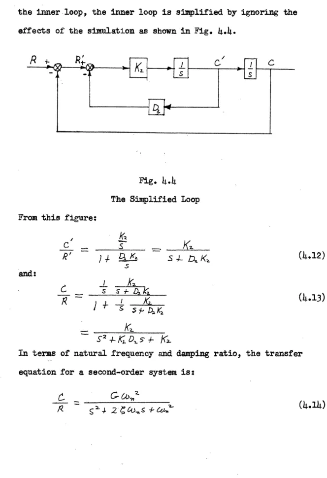
The Control System ... The Simplified Loop ...

Simplified Outer Loop .

...

The Actual Inner Loop . . .

..

Damping Portion of the Outer Loop

Root Locus of Damping Portion of

Outer Loop .. ...

The Entire System ...

Root Locus of Entire System . . .

PACE Computer Diagram ...

Computer Results ... ...

...

63

. . . 67

... .69

...

70

.... . .

71

...

73

...

74

...

73

.. . 75 ...

.*.

77 . . . .* . 79,

Table No.

Effect of Parameter Errors . .... . 81

ix 4.1

Page No.

4.2

4.3

4.4

4.5

4.6

4.7

L.8

4.9

4.10

4.11

4.12

4.1

80

DECLAsSIIFTD

OBJECT

The object of this thesis is to form the preliminary design of an interceptor rocket system that is capable of achieving a successful interception with a mMnum of required weight. It is submitted that this objective of accuracy plus mnumn weight is adequately fulfilled by a one-stage rocket that is controlled only during burning, after which it is left to coast in free fall to the target.

CHA~ssFRII

INTRODUCTION

The subject of this thesis is an anti-missile interceptor

system, which, in turn, forms a part of a submarine-based

anti-missile defense project. The over-all project is described in

this chapter in order to provide the background against which the

interceptor

system

can be intelligently

discussed.

Once the

over-all project has been given, the remainder of the chapter is

con-cerned with certain general characteristics

of the interceptor

system itself, namely, its relationship to the entire project, its mission requirements, and the factors aftectng its design. The

operation of the proposed system is then briefly summarized pre-paratory to the detailed discussions in the following chapters.

1.1 A Description

of

the Over-all

Project

The object of the entire study is to investigate the feasibility of using a submarine as a forward base for an anti-missile defense

system. The possibility was first suggested by the M.I.T. Research

1

Laboratory of Electronics. As the defense system was originally

conceived, the submarine would be stationed near the enemy coast.

1_{MIT-RLE, Internal Report No. 18.}

-From this vantage point, long range radar carried on board the

submarine would be capable of observing and tracking a threatening

missile soon after burnout. From the tracking information, the trajectory of the enemy missile would be predicted and an anti-misslle launched to intercept and destroy the enemy missile.

However, certain dtficulties were encountered in this

originally propose system, Study results of a radar that could

be mounted on a submarine indicated that the tracking of an

object with the reflective area of a warhead would not be possible. The only object that coulo be tracked would be the missile tankage

before it was exploded. Since the separation velocity between

the warhead and tankage could not be determined, the trajectory of tne warhead could not be predicted accurately enough for a success-ful interception.

Because of this flaw in the original proposal, a change in emphasis was made. The primary advantage of the originally con-ceived system was the circumvention of the necessity for dlscrim-inatiug between the warhead and any decoys that might be traveling with it. It was hoped that the target could be tracked and inter-cepted before tne cloua o decoys had grown to sufficient size to require discrimination. However, since the objective of avoiding discrimination appeared impossible to attain, it was decided to

determine

_{if a forward-based system could be used to advantage in}

the discrimination problem itself'. The advantage of a forward-base

is that more time could be used in the discrimination process than

in a system that must accomplish this process in a few seconds at

the terminal end of a hostile trajectory.

With this change in emphasis the operation of the system was modified. The system would again track the tankage and predict

its trajectory. Instead of then launching an anti-missile so as just to intercept the path of the enemy trajectory, it would place a vehicle in an orbit coincident with the target complex, as shown in Fig. 1.1. From the vantage point of a near orbit, it would

use some discrimination technique to eliminate most of the particles in the cloud as not being the warhead. It is proposed to destroy the remaining particles by small auxiliary rockets.

Two discrimination techniques were suggested.2'3 One would use infrared techniques and the other would use a radar method. To use the infrared method the vehicle would be placed in a trajec-tory slightly below the target complex. All of the particles in

the cloud would be observed using a very high quality optical

infrared system.

From studies that have been made on the dynamics

of tankage fragments,4 it is agreed that the tumbling rate of

tank-2

MIT

Inst. Lab. Report R-280

I3

MT

Inst.

Lab.

Report R-321

4 Bendix BPO 867-3, Vol.

ECL

LI4

'4

0Z

C

*S o

I i

! -I

(f ,s 1

's;

_i-i I

EF-TI en

£o

Am_qD :4

og

gri

e₄ ri rie 0 w .3t 4 H ?pq 0 ., 13 B ·s; 4 is ·e . j .= ·;-= oi " i; *L t 4.; a.tT u cc- 2 a·;· = ·r, ? C r ·r. yz r: 5 r. ·-· plJ:,__

DEcaSsmo

age fragment would be an order of magnitude larger than that of the

warhead. Since most of the objects in the cloud would be tankage

fragments,

they

could

be

eliminated by observing the frequency of

their infrared emission.

The radar technique that was suggested would require that

the

vehicle

be placed

as

nearly

as possible

in the same trajectory

that the tankage would have had if it had not been exploded. For the purposes of explaining the radar discrimination method, it is assumed that the distance of a particle from the point where the tankage would have been is approximately:

R=

/A

it

#

Z, )

where R is the range rate and t_o is the time the particle left the

tankage. It is then seen that the quantity R/R, measured for a

particular particle from the point where the tankage would have

been, gives an indication of the time since that particle left the

tankage. It is assumed that the warhead is separated from the

tankage soon after burnout and that decoys may be ejected.

When

the warhead and tankage are at a safe distance, the tankage is

exploded to provide more decoys. With the assumption that the

warhead-'was one of the first particles separated from the tankage,

most of the objects in the cloud can again be eliminated as not

being the warhead by measuring their range-over-range rate. This

range-over-range rate is complicated by the variations in the

gravity field, but the basic principle is still the same.

i~~~iii~~~NWi~~~

1.2

Description

of the Interceptor

I

c

eI

stem

The interceptor rocket system, which is the subject of this thesis, is responsible for the final destruction of the targets. The operation of the system begins after the targets have been

identified by other parts of the over-all system. It first tracks

the targets, then launches a rocket to

destroy

each

target.

The

parts of the system include the actual rockets, a launch mechanism,

radar, computer, and inertial

reference equipment. (The radar,

computer, ana inertial

reference

equipment

are

used

for other

functions in the over-all system.) It is assumed, for the

pur-poses of the design to follow, that there be 6 targets that need to

be destroyed.

1.3 Design Considerations

One of the most stringent requirements imposed on the design

of the interceptor rocket system is

the

weight

limitations.

In

the over-all system, two stages of the anti-missile are used to place the vehicle in a trajectory that intercepts or is tangent to the enemy trajectory. At the point where the vehicle comes in

contact with the enemy trajectory, a booster stage is used to put

the vehicle in the coincident trajectory. Achieving this

coin-cident trajectory requires a very high propulsive capability. In

a sample problem that was simulated on a digital

computer, the ratio

of payload weight to initial

weight of .011 was required.

In

other words, for every added pound in the vehicle,

98 pounds would

DECLSSLSED

If

have to be added to the initial weight of the anti-missile. The interceptor rocket itself has a payload ratio of .31. If 6 rockets

are carried, then for every pound that is added to the

payload

of

each of the small rockets, 1740 pounds are added to the weight of

the

missile.

Since

it is proposed to carry several of these

missiles in a submarine, it is desirable to make the interceptor

system as simple and light as possible.

1.4

Formng

the Basic Design

In forming the basic design, the two necessary components of the rocket, i.e. the warnead and propulsive unit are first considered.

It is then determined what minimum equipment must be added to

complete a successful interception.

The weight requirements demand that the warhead have as

high an energy concentration as possible.

This would call for

some type of small nuclear weapon. The weight of the propulsive

unit depends entirely on the weight to be accelerated and

the

velocity requirement. The velocity requirement, in turn, depends

on the tmne of flight desired. Since the miss distance depends

on flight time and the size of the warhead on miss distance, there is a relation between the weight of the warhead and the weight of the propulsive unit. Because of the highly classified nature of the data on nuclear weapons, no attempt is made here to optimize

this weight trade-off.

For

the

design

purposes

of this thesis it

is assumed that the warhead weigi

50 pounds and has a destructive

radius of 200 feet.

DECLASSIED

DECLASSIFS

The rocket must be launched with an angular accuracy of one

milliraidan.

Since an unguided rocket could not be launched this

accurately,

some type of guidance equipment must be added.

Two

guidance techniques are considered here. The first method would

use a small second stage that would employ some sensing device

(infrared, radar, etc.) to home in on the target at the end of flight. The second method would control the rocket only during burning by command guidance from the vehicle. These two methods

are now compared to see which woulc be best in this application.

The primary disadvantage of the first system is its weight.

Each rocket would be required

to

carry

a sensing

device

plus

the associated instrumentation and control. system. An additional

propulsive unit would be needed to make the necessary correction

at the end of flight. There would also be a problem o target identification. Some assurance would be needed that the second stage homed in on the correct particle. Furthermore, for the homing operations, the attitude of the rocket must be controlled. This would require inertial reference equipment and a reaction wheel or gas jet attitude control system on each rocket. The first system is more accurate but requires a considerable amount of extra equipment.

The second system, on the other hand, would require almost no extra equipment. All that would be needed to control the rocket by command from the vehicle would be a radio receiver, control vanes

DECLASSI ED

in the rocket nozzle and the associated servos and electronics. The command guidance would automatically stabilize the rocket in

pitch and yaw. The rocket would also have to be stabilized in

roll. This would require one small gyro. The rocket coasts in free fall to its target after burnout so no second stage rocket or attitude control devices are needed. Since there is no correc-tive thrust at the end of flight, the position of the target has to be known very precisely rel-ative to the vehicle, the launch direction has to be calculated exactly, the burning characteristics of the rocket have to be very near the design values, and the

command guidance has to be accurate. But if it is possible to achieve these needed accuracies, the command guidance system

would be the more desirable of the two since it would be the lightest and least complicated. The command guidance is then the one

chosen for the interceptor system designed in this thesis. The errors are analyzed to see if it indeed is capable of performing

a successful interception.

1.5 The Operation of the Interceptor Rocket System

The operation of the proposed interceptor system is divided into three phases: (1) the tracking phase, (2) the computation phase, and (3) the launch and guidance phase. The sequence of phases is shown graphically in Fig. 1.2. During the first phase

a specified target is tracked for 20 seconds, with the position

data taken at one-second

intervals. The position data is referred

1.41

ilis~rglMrl

DECLASSIFIED

4K kL Q, a5 J4₄i "t

4.

40 LU A

U

LU ½Q

I

to

0

a):

Q.

-. -r

DECLAsS-SD

-4 .1 I a,. '': I. N.

.I

21nE I 0 -Q. U4 La.

I-q3

:r

0

C: Lu 1*-zt kZ

LASIFID

to an arbitrary non-rotating co-ordinate system fixed in the

vehicle. During the computation phase the tracking data is used

to predict the target trajectory. From

the known

characteristics

of the interceptor rocket and its time of launch, the position of

the rocket is known as a function of

time

and launch direction.

At the instant of interception the rocket and target will be at

the same position. By using the equations giving the positions

of the rocket and target as functions of time, the flight time

and launch direction

can be found.

Launch equipment on board

the vehicle place the rocket in the proper orientation for firing.

At a specified time the rocket is fired.

During burning the

rocket is tracked by the radar. If the rocket deviates from the

desired direction, a command

is sent to actuate the control vanes

bringing the rocket back to the planned path. After burnout the

system begins the same process for the next target.

The most

distant target is intercepted first to keep interference from

the exploding warhead at a. minimum. A functional diagram of the

operation of the system during the tracking and computation phases

is shown in Fig. 1.3 and during the guidance phase in Fig. 1.4.

12

DECLASSIFED

t--a.fr'

ill

1 :: ' . ... -. MOMWWM

Fig, 1.3

Operation of the System During the Tracking

and Computation Phase

'Fig. 1.4

Operation of the System During the Guidance Phase

13

) ( )

2-.o U0 uilay oI eUL.Ub

DECLASSIiFED

The results of the study that follows show that the proposed

rocket interceptor system is feasible. It is found that the

accuracy required to predict the position of the target could be

achieved by tracking the target ifor 20 seconds and then smoothing

the tracking data by the least squares method. The position of the target as a function of time is approximated by the Taylor

series. The results indicate that tne third term, caused by the variation in the gravlty field, is needed to achieve the desired accuracy. The fourth and subsequent terms are negligible. The

design characteristics required for the rocket itself are reasonable. The rocket could be built with the present state of the art. A

command guidance system that only controls the rocket during burn-ing is sufficient to brburn-ing the rocket to within the desired

distance from the target. A second stage is not needed to make corrections at the end of flight. These results are shown by an analog computer simulation of the guidance system.

iJ)r

CHAPTER II

DE.IVATION OF EQUATIONS

FOR THE TRACKING ANID CQMPUTATION PHA6S

The equations needed in the tracking and computation phase are derived in this chapter. The discussion is developed as follows: () The equations of motion of the target relative to

a co-ordinate system centered in the tracking vehicle are

formu-lated

and analyzed using the Taylor

series;

(2)

The method

of

least squares is adapted for use in smoothing the radar data;

(3) The launch

direction

is then

calculated;

(4) Finally,

two

sources

of error in the launch direction vehicle are investigated.

2.1 The Equations of Motion

As stated above, the Taylor series will be used to describe the motion of the target relative to a vehicle-centered, non-rotating, arbitrary co-ordinate system. The motion will be des-cribed in the non-orthogonal directions x, y, z, shown in

A r r - -o

2

1r

X

Fig. 2.1

Co-ordinate System Used in Developing the Equations of otion

It is assumed that the coordinates of the target as a function

of time can be written in the following form:

X X,

X

(t - t)

2.

- 4t,)4

X (t - t)

6~

L ,.

-(2.1)

r r

)( (

- t

rn

±

w

(o-

qt$) (t

6

-

J)3

4

where C

(0

) ',,

' r

)

are constants evaluated at time t

=

t

0

1i6

L E

I

-2.2 The Efect of the Variation of the Gravity Field

To determine the nature of equations (2.1) the constants involved are evaluated. The constants in the first two terms

( X< Yo/

O

o) ~o~ ) represent the target's position and velocity at time t to These constants can be derived easily from the radar data. The constants in the third terms represent the

acceleration of the target relative to the vehicle. In the non-rotating co-ordinate system shown in Fig. 2.1 the only accelera-tions will be those caused by the gradient of the gravity field. In other words, because both target and vehicle are in free fall, the only acceleration of the target relative to the vehicle will be that caused by the difference in the pull of gravity on the

target and vehicle. The acceleration of gravity is:

(2.2)

- 2 C

where: is the gravitational acceleration vector defined

positively down

K is the gravitational parameter of the earth

R is the magnitude of the vector from the center of the earth to the particle.

I6 is a unit vector in the G direction, which is the

negative direction.

The change in G between the vehicle and target is given approxi-mately by:

KR A

-2K

A

R

1G

RY

K 6

K-.

"

~P

I §" T 2 • A F ? J

The geometric relationship of

TARO ET

GT

AG is shown

in Fig. 2.2 to Fig. 2.6.

2

X X L/ ICLe TV CAd TE7?

Fig. 2.2

EARTH

The Variation in the Gravity Field

18

A

G

=

_(2.3)

4. .1 , IZ C

Since the purpose of this development is to determine the nature of the constants in equations (2.1), there will be no loss in generality if equation (2.3) is restricted to the plane of the trajectory. Also, for this development, define the x, z plane of Fig. 2.1 as the plane of the trajectory. Define rotating co-ordinates ( x', z') with z' alongf , as shown in Fig. 2.3.

Fig. 2. 3

Relationship of Co-ordinates to the Trajectory

Then:

(2.L)

A"1,

as shown in Fig. 2.4

Y Fig. 2.

Definition

of

R and

A4:

_ SI R

Ix'

(2.5)

T

1GV R v, I J¢ ? I-,_r, '5 20 -1 X

Equation (2.3) is then:

L\ ;=--

R

3

R

(2.6)

where:

T t and ' one unit vectors in the x' and z' directions.

x Z

't is equal to minus T .

The geometric relationship ofG is shown in Fig. 2.5.

G

c

T

R

3 !

V

Fig. 2.5 Geometric Relationship of AG

To provide some conception of the size of these acceleration terms, they will now be evaluated for a typical situation. It is

D cL·ss1lD

DECLASSIfED

assumed that a typical

trajectory

has a 6000 n. zi. optimum range.

The other parameters can be calculated on the basis of this

assump-tion:

b

= rctn

X

7

e

=

0

°O

4

_{Cos 1}

-

-

CS2 F--

, 3

o

}

-R = ,7 X X /0 2.- s

--

1l/

X/O';

I0

~S.c

If a maximum

separation velocity of 200 ft/sec is assumed between

target and tankage and if it is also assumed

that interception

takes place approximately

IOO1

seconds after separation, then:

- 2

oo

oo

pt

Thus the maximum

vaLue / G will be:

- (Gj(/L/ /O9(2,3 X/a6) =

Equations (2.1) must predict the position of the target for

approximately 60 seconds. The magnitude of the third terms could

then be:

(2.7)

235( C#S 4

which would definitely be significant.

The third terms in the

expansion are therefore needed.

The constants for the fourth

terms

in the expansion represent

the rate of change of acceleration with respect to inertial space.

This will be the rate of change with respect to the rotating

(primed) co-ordinate system plus the acceleration times the angular

rate of the primed co-ordinates.

If:

Gi3

-

c ,

)

(2.8)

Then:

4-L

+

X

(2.9)

Kr-

tic·

o b,2sg

l

)

(2.10)

The angular rate of the primed co-ordinates is the rate of

change of f, which is given by:

=

K

(2.11)

and is perpendicular to A .

Thus:

K

(2.12)

Then substituting equations (2.10) and (2.12) into equation (2.9):

,In

bA

I

-

2c s

(2.13)

P3

-

$/t t -- )

The magnitude of each part of equation (2.12) is now estimated to determine the importance of the fourth terms of equations (2.1):

I

.

I

r

-

2 cos' ,4/

(2.14)

--

|2 Rk

--

¥4

R I3 - 7)

With -= 200 ft/sec and R = 4.14 x 103 ft/sec, the first term of equation (2.14) is:

/,

41

.Y/

/6

)

(- 06) - ('?,2 ' ' O /

(3)7

X

/ q/

_(.2,

z(qt

₄

')C, 5

_{/ Xo7}

_/C

o

{

/?

7 7

A '16-

)

/, 9

/O

-" , 7/s

The components for the second term of equ

- 7 (2.

s/

X., o Y/ ")

9 z

(2,

5 /

/O

17)2

tation (2.14) will be:

-=

75X O

-3 r5(.6)

(2.16)

24

2

(2.15)

da,

R

3)6

/ y

,_4)-a~,

/73

3 )(,

~

K rn'

_C-?

_-i'

)co-r

_?"

_f,.

_{2 --/;7 '}

·

₂

< 2

Ik

R -3 3

KCr

/3

R 1 I uX_; .I

The

term results from the component of velocity of the vehicle

perpendicular

to the

line

of sight between the target and vehicle.

If

it

is

assumed

that the target was ejected radically from the

center, the only perpendicular component of velocity is caused by

transverse acceleration. As can be seen from Fig. 2.5, this

trans-verse acceleration is greatest when Kfis approximately 300 and is less than max. Then the transverse velocity is less than:

2R = i

t-

/ o

~Se~C~

~(2.17)

z~

r

Hi ~:/*2J

5

Xic"

6

)do"

O6

¢

-

/

7

F,

M

(2.18)

The components for the second term of equation (2.l4) is:

r - / A//ec] ato e

3'

The fourth terms of equations (2.1) after 60 sec will be

propor-tional

to:

cLt

CG

91

x

'.oO/

X/o-)

(2.20)

Thus it is seen that the fourth terms of equations (2.1) are negligible and that the first three terms o the Taylor expansion is all that is needed.

In practice, the acceleration terms.would be determined by the

radar data and are not derived by the relations given above.

This

eliminates the need for knowing the orientation of the co-ordinate

system with respect to gravity.

2.3 The Method of Least Squares

The radar on board the vehicle will track the target in the

arbitrary non-rotating co-ordinate system in the spherical

co-ordinates (

,

a,

f).

The information is then transformed into

(x,

y, r) by:

X

r

s

OS

/

(2.21)

If the measurements

made by the radar were exact, the constants

o,

X

, r ,

o

Y,

*

could be solved from equations (2.1)

with three position fixes. Since the radar data will have randumn

uncertainties,

redundant measurements are made. From. these data

ibest values" (

.j y.

, y.

, '

)

are

found

by the

least

squared error method.

These "best values" are found by minimizing the sum of the

squared errors. These errors are the difference between the

measured value at a certain time and the value predicted by

equations (2.1) using the "best value" censtants. Taking the r

equation as an example, the squared error would be:

~E- .-

i); 2t-

(

- jL

,

,

. (r

-

r) .) (2.22) 'Where n is the number of measurements made and:

r,

=

-h

rd.

-Ar

4f

-b

2 _2r

-

bi -_, 6j ( -46

(2.23)

The mean squared error will than be.

E 4

cr,

-(,

7Li - go+ oC2_a

+=

zEiJ_

_(2.24)

''.

r

-Cry-

4

rO

(it,

-

)

,t

-eo

g

Z

To minimize this mean squared error the partial derivatives with

respect to the three constants ( r, _{Y_ )} , _- r- _. ) are set equal to

zero:

E

, ,

--

Ir.

(

-t- i

₂

7--.

7-I,

,-.-4)_

-P2

5r

-

f

4 - ,)L

,n2 S.'IU , t2 ·

c '1

·.

_ ( -

rL,

Lt-

_

t

-t-r-o

~ ~

. 4

_'Z

-

t

_--

_.)

=

27

+

n C

t; - io) t

(

-

i)t

-4 T ,, Z O

( t,~

-

ib)

1^

r- _s~~

-r

( t, - t) '

2

r

_/-'

z

,

2

)r

-

(% + 4 (- ₂ t)

r

Z

,

,-#7

2D-(Y~

-Xt)-it

-Vt-t)#

_X

_

O

-

2? r -

+r,>

4

-2 r r

r.

+

7;11

71~e (-, ( t~ - ') - ,7 -2

This results in three simultaneous equations 'or the constants:

4-

ti-

_{2 °} r -p.,

'

i

- I

(2.26)

I

p)3\

4 ~

ti

~.)

Y-2 3

.

(ti-i")

x

,l A

2=r~~~~~r

2=1~

~

2~

The notation can be made more concise by using matrix notation.

If a matrix A is defined as:

A

/ ~(,

-

) •(

2

I (E ia . C,7-t~.

/ (i -i")

28 (2.25)

.

,L

2

'rf

- c6

L

7

-/

~t

2

Zr

2>

ci-z-

tY)

Z-, 2

(2.27)

( Z- - 2j (- - 4

-1 EE

)] (t-, - 2i.)

rz-

) I

Z

'Z-- _, _

")OL

Z

2-1.-I\

ra(t,-io--

-- 11C~

n6 -- -

L-- ---

-

t)2

2

2 2 Al Z= rz

j

r- r.Zr Z-=/~"

Ct -. ) -r

114 I/~

·Equations (2.26) can be rewritten as:

AAR=

A

T

R

(2.28)

where R is a colmina matrix consisting of the measured values:

R-"5<

(2.29)

and Ro is a colvmn matrix consistzng of the desired "best values":

₀

PC

IZ\0 r7-I4~_{L 6 J}

C

=

A

-'A-(2.30)

A

(2.31)

then the desired values will be

R,

P=

R

Also, for the other two components:

Xo= C

.X.

Y

-

Y

Y,.

%o-

29

(2.32)

where:

(2.33)

(2.34

If:

anli Y, YL t I I

(2.35)

The matrix A and thus C are precalculated constants that depend

only on the number of fixes and the time between fixes.

The time

between fixes is picked.as one second. The number of fixes will

depend on the accuracy required. It is desired that the position

of the target be known within 200 feet after 60 seconds. This

will require that the velocity constants be known to within 3 ft/sec.

Because of the nature of the radar, the angular measurements

will

be the most critical. If the distance from the vehicle to the

target is approximately 200,000 feet, the required accuracy for

the angular rate is 1.5 x 10 rad/sec. The number of fixes

needed at a rate of one per second is approximately 20. This

will improve the accuracy by approximately:

=Cry

(2.36)

where o- is the deviation of one measurement,

EG

is the deviation

of "best value" if there are n measurements, and n is the number

of measurements. With an assumed accuracy for the radar of .001

radi;an, the accuracy of the "best values" will be:

00/=~*

t(2.37)

l~k

30

Y-Y

X,1

X3n Y

::

! _

With a tracking time of 20 seconds, this standard deviation will

give an angular

rate

deviation

of:

t~c

=

20,z/ _/1

=

) /

/S G(2.38)

~/so

which

is seen to be within the required tolerance.

2.4

The Calculation

of the Launch Direction

At the end of the tracking period, all necessary information

is available for the calculation of the launch direction. The

launch direction is calculated by deriving the equations for the

position of the target an mfor the attacking rocket as a function

of

time, with time

t

=

0 at

the time the rocket stops burning.

The position of the target and rocket are then set equal to obtain

the time of flight

and

launch

conditions.

All time intervals in the operation of the system until

rocket burnout are constant and are determined by design

considera-tions. After the system receives a command to destroy a target,

it tracks the target for 20 seconds as described above. After

this, there is a time period in which the computer solves for the

launch conditions and the vehicle prepares to launch the rocket.

Then at a given time from the initiation of tracking the rocket is

launched. Since the rocket is designed to burn for a definite

period, the time of rocket burnout is also fixed relative to the

initiation of tracking. The position of the target relative to the

vehicle is known at rocket burnout.

The position of the target as a unction of time after

burn-out is given

by equations

of the same form as equations

(2.1).

If tme t is

picked

as the burnout

time,

the

constants

for

equa-tions (2.1) will be given by equaequa-tions (2.32) and (2.33).

The

elements of the A matrix will then be defined by the time

val between the beginning of tracking and burnout, and the

inter-val between fixes as described in the previous paragraph. If

time t = t is arbitrarily set equal to zero, the equations for

the position of the target will be:

A

'

X'T

=X 4

)io t rL If tz(2.39)

+

The position of the rocket at burnout is determined by the

design of the rocket and the launch direction. It is assumed

that the rocket accelerates approximately in a straight line.

Then the velocity of the rocket in the * direction at burnout is:

0rn

atj

he

(2.40)

and the position is:

7on

F

jr

T

T

t

ch)

L

a!

t

(2.41)

O

The acceleration as a function of time can be found experimentally

through static firings of the rocket. The accuracy requirements

for these constants

and

the design

of the rockets will

be discussed

later. The initial conditions in the other two directions are:

Xo0

"

=

,,,

,.

~

's

(2.42)

Yon

where

,

and

Y

shown in Fig. 2.i

= Y- C s 'L n

9

t on COS 53 I,

eL are the launch angles these relationships are

6.

IIr_

X

AL

V

Geometrical Relationships at the Time of Launch

After burnout the only accelerations of the rocket are those

due to the difference in the gravity field. They are of the same

nature as the acceleration acting on the target as described in the

first section of this chapter. The acceleration of the rocket

is proportional to:

/

E3

(2.43)

where t- r=, , i . Since the acceleration caused by gravity

is itself a first order effect, any first order effects on it

can be neglected as second order effects. Thus r can be neglected

compared to 7T t since ,, represents only about 10% of the total

flight path. The acceleration is then:

r

-R'

₀

3

(2.44)

and the displacement at the end of flight is:

!Ka,

i

(2.45)

where tf is the time of flight. The acceleration of the target is:

a th

_d

slen

(2.46)

and the displacement

is:

a

rr

ks, t

_(2.47)

Since

to

t

is approximately

r~,

the displacement of the rocket

is:

A~l

r -c)

2

A'

r,'

r

3/?'

2-

3R'

z

3

(2.48)

Thus the rocket acceleration is approximately one-third the

target acceleration as derived from the radar data.

The equations of motion for the rocket are:

XR

=

Y

T

,

-r +

r

3

t) Svn

c

9

S

(-2.49)

3 2f

To

fnd

the launch condltions, set

equations

(2.39)

equal

to

equations (2.49). The time of flight is solved

from

the r equations:

-L-6

r

z-

=

T

,

(2.50)

T~o - ~~ =0of O (2.51)

The solution of this quadradic

involves

the difference of

large

nunbers

_{and it also involves a square root which}

akes

its

solution on the computor more difficult. Since the accelerations

A first approximation for the time of flight is,

(2.52)

zI~ I -

-r'" -'

. .

-Then a second approximation is given by:

(2.53)

Substituting equation (2.46) for t, gives:

(2.54)

(ro

- Amp

- r

-r

To confirm the accuracy of this approximation by a typical example:

] :

2 0,

p -,- I A

Oo

\

-C

#

SoC

(2.55)

-o0 - 8

qO

3

Q/95e7

O s

5c-The next approximation would be:

2 j O0

--- 5000 - _{.3 YC o}'?

The error would be .9 x 10 5 which would be very much less than

the errors in the other numbers in the equation.

With the time of flight known, the launch direction can be

solved from the other two equations. From the x equation:

ZX

-Xv I<\

i

-/-

n~t

.

= ><R

- (ro + <,,~

t;)s/'>?66

'k" + Yr tf

_Y-r

Y.

_z

_R

.)·S-/ 1,7 , _4;

~~-

t

(2.58)

36

(2.56)

(2.57)

Y- -₀ -r- ₀

.

7-t

~-

-

-",

~

"=

-

/,

-

';)

se

- A 4 2

BL

=

SIYI

_(2.59)

2,~).

From the y equation:

Yr Y.

L /

tF 4

Y

=

,+

d

os.s^

4 Y-, -fE'

(2.60)

-,So -,- yo - :t . . (2.61)

(r,

4

)Cos S

2.5 Error Calculations

Two different sources of error are investigated here. These

are the error in position caused by an error in burning time and

the error in position caused by an error in final velocity.

One of the most likely sources of error is an error in burning

time: Burning time is dependent on the initial temperature of the

propellant which is difficult to control. If the actual initial

temperature differs from the design value, the fuel will burn at

some

rate other than the design rate, but since it is likely that

all the fuel will be burned, the rocket will reach approximately

the same final velocity. Thus the primary effect of an erroneous

burning

rate will be an error in the initial position of the rocket

( r,

) and in the burning time

( t

).

To determine the effect of an erroneous burning time, the

error caused by a 10% slower burning time is calculated.

It would

take approximately a 50OF

error in initial temperature to cause

an error this large in the burning time. Thus it is probable that

the burning time can be held well within this 10% tolerance.

In

these calculations the primed quantities are the actual values and

the unprimed quantities are the design values. Also, the gravity

accelerations can be neglected in these calculations as second

order effects and the acceleration of the rocket can be assumed

constant.

For this example, let:

.~$

=

/o

Se.

(2.62)

r

=

S

as

Fso

Since the acceleration of the rocket is assumed constant, the

design acceleration is:

t_

0

=

-f/SeF

eo

(2.63)

and the actual value is:

/j

-____~¢£ - (2.6h)

The design value for the initial position of the rocket is:

ro

77

_-Z

2,i -.

₂

C

₂₆

(2.65)

and the actual value is:

/

₂

F

on5 = r/ 7, uo,

2 ?

F-t (2.66)

The effects of these errors combine to produce an error in the

calculation time of flight. The calculated value is:

3

2

c

e(2.

6

₇₎

I

.

? - 7

.

i

'r-7;

O

/_

o

0

-

j

o o

I

A-

7;

65660 - z o

The actuai value for the time of flight is:

A~~~~

Cc'I - YTo,

-9 Y 4 - r

/25

00oo-

7 -oo.

7

?3

_2

(2.68)

500

ooo -

2

The miss distance can be found by refering

to Fig. 2.7.

R.

T

d

,

.E

', Fig. 2.7

Miss Distance

39

At the calculated interception time the target will be at position

T1, at the intersection of the target and rocket flight paths.

Although the rocket was launched at the correct time, it accelerated

slower than planned so it will be at the position PL at the

cal-culated interception time. At some time later the rocket and target

will be at positions R2 and T2, respectively, which is approximately

thefr closest miss distance. The time interval between the

cal-culated interception time and the time when the rocket and target

are at positions

R

2

and T

2

is the difference between the actual

and designed rocket burning time plus the difference in time of

flight from burnout as shown in the following equations:

p

(*jit

-

a

t_

)4

(2.69)

(i -o) (3O2

-3

-,

62

Thus the difference between the position of the target and rocket

at the calculated interception time is:

Pk

4,

2

-

-T

ot

o

St

-

r6

(2-70)

-

(&C

-2'

2 O6

C

C)

Sec

-Z

3 o

Fft

At a time interval St later, the rocket and target pass at

approximately the closest miss distance. If the velocity in the

transverse direction is 187 ft/sec (See equation 2.17) the minimum

miss distance is:

c), = R?1 7

-

r ;

~-

C2,~)6C,77 -

7

'=

'0

(2.71)

If the weapon is detonated at the calculated interception

time, the rocket will be well

outside

the

planned

tolerance.

However, the weapon could be detonated within the required accuracy

by a proximity fuse.

This possibility

will not be considered

further here.

An alternate means of detonating the weapon could be

by command

from the vehicle.

The vehicle would recalculate the

interception time by using the actual velocity and position of the

rocket as measured by the radar. The radar will measure the

velocity and position of the rocket at approximately five seconds

after the planned burn out, at this time the rocket will have

burned out. The values of velocity and position are inserted

back into equation (2.54) to determine the new interception time.

This time is relayed to the rocket, and a clock detonates the

weapon at the proper time.

The other source of error considered is an error in final

velocity.

This error can be caused by chunks of fuel breaking

off, by erosion, by residual fuel, etc. The effect of a final

velocity

error

on

miss distance are readily calculated.

If a 2% error in final velocity is taken

in time of interception will be:

= m/7m

s006 -2 t-

7n

L

-y

2o

2

-

31/,/S -3/2s-'

-=

The minlimum miss distance is then:

as an example, the error

(2.72)

(2.73)

Thus it is seen that with reasonable tolerances of 10% on

burning time and 2% on final velocity, a launch direction can be

calculated that will bring the rocket to within the required

dis-tance from the target.

It remains to be shown (Chapter IV) that

the rocket can actually be launched along this direction.

42

1^ 7-, - r"'? 0 1_.

Y_0,7

T

- 3/,2EO5

d;

vSt-

=

/ 9-

~X, 6,-

=

12 I/

CHAPTER

III

PHYSICAL DESIGN OF TEE ROCKET

In this chapter a rough estimate is made of the important characteristics of the actual rocket. A velocity impulse is

chosen to satisfy the requirements of the over-all system.

Estimates are made of the weight of the payload, structure,

and

other equipment, and a fuel is chosen. A burning time is selected

that fulfills the time requirements of the control system. All of

this

material

is combined

to determine the mass ratio of the rocket,

the configuration of the propellant grain, the characteristics of

the nozzle, etc. From these are found the weight, dymanic

charac-teristics, acceleration, etc. of the rocket.

3.1 Design of the Rocket Motor

In designing the rocket the weight of the warhead is assumed

to be 50 pounds. The actual design of the warhead would involve

highly classified information and also would be beyond the scope

of this thesis.

If the actual weight of the warhead should differ

from the assumed weight, all other weights and design parameters

can be changed by a proportional amount. It is also assumed that

the control system weighs 10 pounds and that the structure accounts

for 15 per cent of the total weight. It is desired that the

max-iLum time of flight be approximately

40

seconds. Since the target

could be as much as 200,000 feet away, the desired velocity

impulse

is 5000 feet per second.

The fuel chosen is ammonium perchiorate ovidizer with

poly-butadience fuel binder and aluminum additive. The characteristics

of the fuel are:

I @1000 psi 250 sec (at sea level)

sp

Burning rate @1000 psi .467 in/sec

Burning exponent, n .236

Density .063 lb/ft3

Since the specific impulse at sea level is expected to be improved

to 260 seconds in the near future, this number will be used in the

design. The ideal exhaust velocity at sea level can then be

deter-mined from these fuel characteristics:

=(260 secY32.2 ft/sec2)

= 8380 ft/sec

From this ideal velocity the characteristic parameter of the

fuel, arbitrarily called K, can be found. The parameter K is

in-volved with the burning temperature of the fuel. The equation is:

_H(7~5t

[

4=

(E

)

jK

I

(3.2)

where

k

Specific heat ratio (assumed to be 1.25)

P1 1000 psi chamber pressure

P2 " 14.7 psi exit pressure

then:

8380 ft/sec

=

_,//s

_2L

thus:

K

=

'

3

o

(3.3)

For convenience in the manufacture and handling of the rocket,

the exit of the rocket nozzle is assumed to have approximately the same diameter as the case. With this assumption and

antici-pating the size of the case and throat area from the results of

the design to follow, the ratio of exit area to throat area is

approximately 54. The pressure ratio can be found from the

relation:

=

___

____________

(3*4)

A

)-

(e

Solving this equation using the graphs in reference ( ), the pressure ratio will be:

-

800

(3.5)

thus the exit pressure will be:

P. 5 /o00 = 1i.25 psi

Using equation (3.2) the ideal exhaust velocity in a vacuum can be derived:

Z frz /

(3.6)

= 8380 5

= 10,050 ft/sec

The effective ehaust velocity is:

C = C) +V'q

IA

(3.7)

where:

P =

a atmospheric pressure

A = 38.6 in2 exit area

e

W = mass flow rate, is anticipated to be approximately 4.2 lb/see

thus:

l(/,'S2

)3s,c)(32. 2)

e

10,050

+ 1 )2

'-2

= 10,050 + 370 = 10,420 ft/sec

The specific impulse in vacuum is then:

I

-=

/0 420

=

324

sec

32.