HAL Id: hal-03093481
https://hal.archives-ouvertes.fr/hal-03093481
Submitted on 3 Jan 2021HAL is a multi-disciplinary open access
archive for the deposit and dissemination of sci-entific research documents, whether they are pub-lished or not. The documents may come from teaching and research institutions in France or
L’archive ouverte pluridisciplinaire HAL, est destinée au dépôt et à la diffusion de documents scientifiques de niveau recherche, publiés ou non, émanant des établissements d’enseignement et de recherche français ou étrangers, des laboratoires
July 2019 heatwaves in Western Europe
Robert Vautard, Maarten van Aalst, Olivier Boucher, Agathe Drouin, Karsten
Haustein, Frank Kreienkamp, Jan van Oldenborgh, Friederike Otto, Aurélien
Ribes, Yoann Robin, et al.
To cite this version:
Robert Vautard, Maarten van Aalst, Olivier Boucher, Agathe Drouin, Karsten Haustein, et al.. Human contribution to the recordbreaking June and July 2019 heatwaves in Western Europe. Journal of Geophysical Research: Atmospheres, American Geophysical Union, In press. �hal-03093481�
Journal XX (XXXX) XXXXXX https://doi.org/XXXX/XXXX
Human contribution to the
record-breaking June and July 2019
heatwaves in Western Europe
Robert Vautard1, Maarten van Aalst2, Olivier Boucher1, Agathe Drouin3, Karsten
Haustein4, Frank Kreienkamp5, Geert Jan van Oldenborgh6, Friederike E. L. Otto4,
Aurélien Ribes3, Yoann Robin3, Michel Schneider3, Jean-Michel Soubeyroux3, Peter
Stott7, Sonia I. Seneviratne8, Martha M. Vogel8, Michael Wehner9
1Institut Pierre-Simon Laplace, Paris, France
2University of Twente and Red Cross Red Crescent Climate Centre 3Météo-France, Toulouse, France
4University of Oxford, Oxford, U.K.
5Deutsche Wetterdienst, Offenbach, Germany 6KNMI, de Bilt, The Netherlands
7U.K. Met. Office, Exeter, U.K. 8ETH Zürich, Zürich, Switzerland
9Lawrence Berkeley National Laboratory, Berkeley, U.S.A.
E-mail: robert.vautard@lsce.ipsl.fr Received xxxxxx
Accepted for publication xxxxxx Published xxxxxx
Abstract
Two extreme heatwaves hit Western Europe in the summer of 2019, with historical records broken by more than a degree in many locations, and significant societal impacts, including excess mortality of several thousand people. The extent to which human influence has played a role in the occurrence of these events has been of large interest to scientists, media and decision makers. However, the outstanding nature of these events poses challenges for physical and statistical modeling. Using an unprecedented number of climate model ensembles and statistical extreme value modeling, we demonstrate that these short and intense events would have had extremely small odds in the absence of human-induced climate change, and equivalently frequent events would have been 1.5°C to 3°C colder. For instance, in France and in The Netherlands, the July 3-day heatwave has a 50-150-year return period in the current climate and a return period of more than 1000 years without human forcing. The increase in the intensities is larger than the global warming by a factor 2 to 3. Finally, we note that the observed trends are much larger than those in current climate models.
Keywords: Climate Change, Heat Wave, Extreme event attribution
1. Introduction
Two record-breaking heatwaves struck Western Europe in June and July 2019. These heatwaves were recognized as the
event took place in the last week of June 2019. The event broke several historical records at single locations, including France, Switzerland, Austria, Germany, the Czech Republic, Italy and Spain. In particular, the all-time temperature record
44.1°C, Conqueyrac) was broken on June 28 by almost 2°C with a new record of 46.0°C, established near the city of Nîmes. In Switzerland, more than 40 stations experienced record daily maximum temperatures for June. In Austria, The Netherlands, Germany and even Europe the whole month of June 2019 was the warmest ever recorded ( https://climate.copernicus.eu/record-breaking-temperatures-june). Such extreme heatwaves usually occur in mid-summer, when they have less impact on school days and professional activities than in June or September. In France, due to the heat in June 2019, the government decided to postpone one national school exam, inducing organizational challenges at large scale. In the hottest areas of Europe, a number of wildfires took place, and train tracks were damaged in Switzerland.
A second short (3-4 days) record-breaking heatwave struck Western Europe and Scandinavia at the end of July 2019. Records were broken again, albeit in different areas. In France, the highest amplitudes of the heatwave were found in Northern and Central parts of the country, with records of either 1947 or 2003 broken by a large departure on July 25. For instance, the historical record of Paris (Station Paris-Montsouris) of 40.4°C became 42.6°C and a temperature of 43.6°C was measured in the Paris suburbs. In Belgium and the Netherlands for the first time ever temperatures above 40°C were observed. In Germany, the historical record of 40.3 °C was surpassed at 14 stations, with one station reaching 42.6 °C (Lingen). In the UK, a new highest ever maximum temperature of 38.7°C was measured in Cambridge. Further west, where the heatwave was slightly less intense, the record from 1932 (35.1°C) at the historic Oxford Radcliffe Meteorological Station (continuous measurements for more than 200 years; Burt and Burt, 2019) was broken by more than one degree, with a new record maximum temperature of 36.5°C. These high temperatures caused hundreds of extra deaths in Europe (see Section 5).
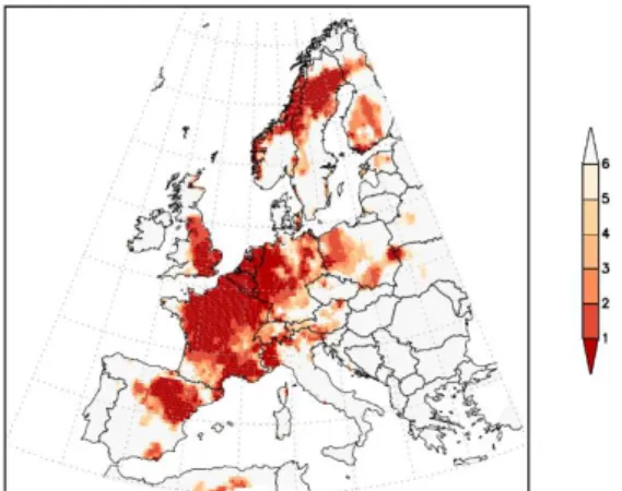
Figure 1: Rank of annual maximum temperatures observed in
Europe in 2019 compared to 1950 - 2018, based on the E-OBS data set (Haylock et al., 2008, version 20.0).
Taking into account both episodes, the spatial extent of broken historical records is large and includes most areas of France, the Benelux, Switzerland, Germany, the Eastern U.K. and Northern Italy (Figure 1). A few days after each of the events, reports of attribution to human influences were made (van Oldenborgh et al., 2019; Vautard et al., 2019a). In this article, we collect these results in a single study to draw common conclusions.
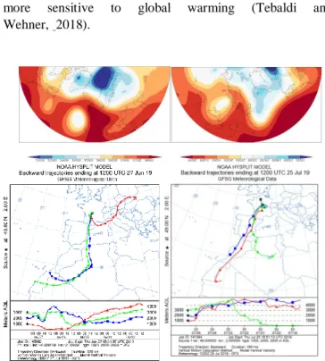
Both heatwaves occurred due to a ridge across western Europe, together with a low-pressure system developing offshore the Iberian peninsula, as shown in Figure 2a,c. These weather patterns induced intense advection of hot air from North Africa across Spain to France as shown by the NOAA HYSPLIT back-trajectories (Figure 2 b, d). Soil conditions across Europe were not anomalously dry prior to the June event, which rules out a large warming amplification by soil-atmosphere feedbacks. By contrast, the July heatwave was accompanied by severe drought conditions in areas such as France, parts of the Netherlands and Germany, which probably contributed to heat development given that dry soils have been shown to cause an additional temperature increase at regional scales due to land-atmosphere feedbacks (e.g., Seneviratne et al., 2010). Interestingly, this may also point to a link between the two events, since the dry soils prior to the July event were largely the result of the June event. A similar mechanism played a role in the twin 2003 June and August heatwaves in Europe, with the June heatwave likely enhancing the intensity of the August heatwave because of its effect on soil drying (Seneviratne et al. 2012).
We present here the results of an attribution analysis following the same methodology used in previous analyses (e.g., Kew et al, 2019, Philip et al, 2018, Otto et al., 2017). We also refer to these studies and van Oldenborgh et al. (2019) and Vautard et al.. (2019a) for a detailed explanation of methods and models.
2. Event definition, observations and trends
In both cases, we use an event definition that illustrates potential impacts on human health, by combining both daytime and nighttime heat and the persistence of the episode as multi-day events have been shown to have disproportionately larger health risks in Europe (D'Ippoliti, 2010). For the June case we defined the event as the highest 3-day averaged daily mean temperature for the month of June each year (TG3x-Jun) and for the July case we used the all-year 3-day maximum (TG3x). The time span of the indicator almost corresponds or exceeds the length of the heatwave period. While the three-day average maximum is slightly lower than the single day maximum, we are expecting it to be
more sensitive to global warming (Tebaldi and Wehner, 2018).
Figure 2: ERA5 500 hPa (upper panels), for 27 June 2019
(left) and 25 July 2019 (right), together with back-trajectories calculated using the NOAA HYSPLIT online trajectory tool (https://www.ready.noaa.gov/hypub-bin/trajtype.pl); back-trajectories are calculated to arrive at 3 altitudes (1000m, 2000m and 3000m) to sample the heated low atmosphere.
For the June case, the analysis is limited to France where it was most intense while for the July case it is extended to several European countries: France, Germany, The Netherlands and the U.K.. These are countries in which a number of temperature records were broken and data were readily availability through study participants or public websites. The locations considered are single weather stations shown in Supplementary Table 1. In both cases we also used the average over metropolitan France as obtained from the E-OBS data base (Haylock et al., 2008). It is close to the value of the official French thermal index (also used), which averages temperature over 30 sites well distributed over the metropolitan area and is used to characterize heatwaves and cold spells at the scale of the country.
The rest of the analysis is based on a set of 6 individual weather stations, with the purpose to make the analysis more concrete for effects at local scale, which is the scale relevant for impacts, and also some of the selecte stations had records with a long history. We selected the stations based on the availability of data, the relevance to the heatwave, their series length (at least starting in 1951) and avoidance of urban heat island and irrigation cooling effects, which result in non-climatic trends. The locations considered (Toulouse for June, and Lille-Lesquin, de Bilt, Cambridge, Oxford,
Weilerswist-Lommersum for July) all witnessed a historical record both in daily maximum and in 3-day mean temperature (apart from Oxford and Weilerswist-Lommersum where only daily maximum temperatures set a record). Further, the selected stations are either the nearest station with a long enough record to where the study authors reside, or representing a national record. Most of these daily temperature time-series have been quality controlled, and do not exhibit major homogeneity breaks at the monthly time-scale. However, no homogenization procedure is applied, as homogenization of daily time-series remains a challenging task (Mestre et al., 2011). As a consequence, breaks related to changes in the measurement procedure can still affect these data, and in particular observed trends.
There is a clear trend in observed annual values of the event indicators in each case (see e.g. Supplementary Figure 1 for the July case stations with TG3x), and the 2019 values represent a large excursion away from the average indicator value which is already a yearly maximum. The trend in observed series is then quantified using the properties of the fit of a Generalized Extreme Value (GEV) analysis with a covariate (smoothed Global Mean Surface Temperature, GMST) representing an indicator of climate change (from anthropogenic and natural factors) on the position parameter, keeping the scale and shape parameters constant.
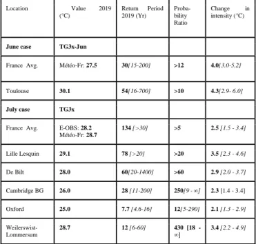
For extreme heat, the GEV has a negative shape parameter, which describes an upper bound to the distribution. This bound is however increased by global warming. If the temperature in 2019 is above the bound in 1900, the probability of the event occurring without the warming trend is zero and the probability ratio formally infinite, subject to the assumptions made and sampling uncertainties. Results for each station are shown in Table 1.
In June, as observed in France at the country scale, the exceedance of observed TG3x-Jun has a current-climate return period of 30 yr (15 to 200 yr) (Table 1). This is roughly 180 times more than it would have been around 1901 (at least 12 times more). The increase in TG3x-Jun since 1901 is estimated to be 4.0 ºC (3.0 to 5.2 ºC). This implies a much higher warming trend in France in June hot extremes compared to that of the average European land summer temperature, which has warmed by about two degrees. For the station of Toulouse, similar results are found.
In July, the change in intensity for similarly likely heatwaves varies between 2°C and 3.5°C depending on the location. The return periods range from about 8 years in Oxford to 80 years in Lille. For the metropolitan France average, best estimates of the return periods are of the order of 130 years, even taking the trend into account. In France,
Benelux and Germany the return periods for individual stations are relatively similar (60-80 years). In Germany for the selected station we find a return period of 12 years. This relatively low return period could be due to the fact that the station is located slightly on the eastern edge of the affected region and the core event was shorter than 3 days. In the U.K., return periods are shorter because the event was in fact shorter than 3 days and 3-day averages there mix hot temperatures with cooler ones. As seen in Table 1, uncertainties on the return period are very large which leads to similarly large uncertainties for the Probability Ratios with many cases where an upper bound is infinite. In a few cases, the best fit also gives zero probability in 1900 thus only a lower bound can be given.
Location Value 2019 (°C) Return Period 2019 (Yr) Proba-bility Ratio Change in intensity (°C)
June case TG3x-Jun
France Avg. Météo-Fr: 27.5 30[15-200] >12 4.0[3.0-5.2]
Toulouse 30.1 54[16-700] >10 4.3[2.9- 6.0]
July case TG3x
France Avg. E-OBS: 28.2 Météo-Fr: 28.7 134 [>30] >5 2.5 [1.5 - 3.4] Lille Lesquin 29.1 78 [>20] >20 3.5 [2.3 - 4.6] De Bilt 28.0 60[20-1400] >60 2.9 [2.0 - 3.7] Cambridge BG 26.0 28 [11-200] 250[9 - ∞] 2.3 [1.4 - 3.4] Oxford 25.0 7.7 [4.6-16] 12[5-290] 2.1 [1.3 - 2.9] Weilerswist- Lommersum 28.7 12 [6-60] 430 [18 - ∞] 3.4 [2.2 - 4.9]
Table 1: Statistical quantities linked to the trend in the
observed values of the indicator.
3. Models and their evaluation
The observations give a trend, but do not allow to attribute the trend to a cause in the traditional Pearl interpretation (Pearl, 1988; Hannart et al., 2016). For the attribution analysis we used a large set of 8 climate model ensembles including the multi-model ensembles EURO-CORDEX and CMIP5, single-model ensembles from the CMIP5 and CORDEX generation (EC-EARTH, RACMO), specific attribution ensembles (HadGEM3-A, weather@home) as well as two single-model ensembles from the CMIP6 generation (IPSL-CM6-LR and CNRM-CM6.1) that were available at the date of study. Supplementary Table 2 summarizes the characteristics of the model ensembles and references. Note that one of the model ensembles, CNRM-CM6.1, was not used in the June case. Extraction of station points is done using a nearest neighbour method unless specified otherwise. As the
grid spacing is smaller than the decorrelation scale for heatwaves the details do not make a difference.
To evaluate these models we test whether the statistics of extreme heat in these models are consistent with the observed statistics. The test consists of fitting the models to the same GEV distribution as in the observations and comparing the scale (σ) and shape (ξ) parameters of the fits to the model data with the parameters of the fits described in the section observational analysis. We do not consider the position parameter (μ) as biases in this parameter can easily be corrected without affecting the overall results. All results from this comparison are shown in Supplementary Figure 2.
In the June case, The EURO-CORDEX and CMIP5 multi-model ensembles and IPSL-CM6A-LR multi-models overestimate the scale parameter by about 50%, weather@home by a factor two. EC-Earth and the dependent RACMO model would pass a test based on this parameter for both the county scale and the Toulouse site. The shape parameter is generally negative for heatwaves, but in France the parameter is less negative than in most regions (Vautard et al., 2019b, Fig. 4). Although the uncertainty in shape parameter estimates can be large, models's shape parameters are collectively more negative than observations'. This induces a positive bias in the probability ratio. Taking the two tests together we find that barely any ensemble passes the test that the fit parameters have to be compatible with the parameters describing the observations, in line with issues encountered for area-averaged heatwaves in the eastern Mediterranean (Kew et al., 2019). We found no evidence of atmospheric dynamics biases, and the cause of the overestimation of variability is still unknown (see also Leach et al, 2020).
Hence, we are formally left for the present analysis with no real suitable ensemble to use for the attribution (though we did not check the suitability of each single CMIP5 or EURO-CORDEX models and cannot exclude that some might be suitable for both parameters). Given this, we decided not to give a synthesis result drawn from observations and models as in previous studies but still proceed with analyzing all models, noting that the results are only indicative at best when drawing conclusions.
In the July case (see Supplementary Table 2), the same conclusions hold regarding models skill as in our analysis of the June heatwave. Models have a too high variability and hence overestimate the scale parameter, sometimes by a large amount (factor 1.5 to 2.5). This is particularly marked for the France average. However, HadGEM3-A, EC-EARTH, IPSL-CM6-LR and CNRM-CM6.1 appear to have a reasonable departure from observations. For the other models the 95% confidence intervals on the scale parameter does not overlap
with the confidence interval on the scale parameter from the observations. For individual stations studied here, shape parameters are simulated within observation uncertainties. The discrepancy for the scale parameter is also reduced except for weather@home where variability remains too high.
4. Attribution
The attribution was carried out using different methods for each model ensemble, and also between the June and July cases, due to the nature of the simulations and the availability of methodologies and production teams in real time. For transient simulations and the July case (EC-EARTH, RACMO, EURO-CORDEX, CMIP5, HadGEM3-A, IPSL-CM6-LR, CNRM-CM6.1), estimations are obtained from a GEV fit with the smoothed GMST covariate as an indicator of climate change and human activities. The training period for the fit is taken as the largest possible period between 1900 and 2018 in order not to include the extreme event itself, as it would lead to a selection bias (see Supplementary Material for the reference periods). For some model ensembles the fit was made over a shorter period as the data were not available back to 1900 (such as for RACMO, EURO-CORDEX and HadGEM3-A). For weather@home, due to the large ensemble size, a non-parametric comparison of the observed event in the simulation of the present day climate with the same event in a counterfactual climate performed. In the June case, the same methods were used except for EURO-CORDEX and IPSL-CM6 where a non-parametric comparison was also made. Despite these methodological differences, attribution is made comparable in all cases by comparing return periods or values for the exact same reference dates (1900 and 2019).
For ensembles where bias correction was applied prior to the analysis (the multi-model CMIP5, EURO-CORDEX), the estimation of probability ratios or intensity changes is made based on events exceeding the observed value of the index. For the non bias-corrected ensembles, the estimation is made based on events with similar return period as in the observations.
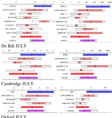
A synthesis is made based on observations and the model ensembles that passed the evaluation by weighting the results for the July case, and based on all ensembles for June, but without synthesis between observations and models due to model/observations inconsistency. For June, for each model ensemble, uncertainty only considers sampling uncertainty (representing natural variability). For the July case, the same is represented, but we also added the “model uncertainty” obtained as the model spread (inter-model variability in the estimate) in addition to each model’s sampling uncertainty (open bars in Figure 3). This allows a more realistic uncertainty for each model result. In the model/observation synthesis (purple+open bars in Figure 3), individual model
results are combined with the observed estimate in two ways: a weighted average (by the inverse of the variances) denoted by the colored bar and an unweighted average denoted by the open bar. Model spread is added to the model synthesis without reduction due to the number of models. The unweighted average thus puts more weight on observations.
We present all results for the probability ratios between the 2019 and 1900 climates and for the change in intensity in Figure 3 for the two cases.
June case
Despite model/observations discrepancies, in June, the observations and almost all models show a large increase in the probability of heatwaves like the one observed in June 2019 (as described by the 3-day mean temperature, both averaged over all of France and in one specific city, Toulouse). For both the average over France and the Toulouse station we find that the probability has increased by at least a factor five (excluding the model with very strong bias in variability). However, observations indicate a much higher factor of a few hundreds. Similarly, the observed trend in temperature of the heat during an event with a similar frequency is around 4 ºC, whereas the climate models show a much lower trend (about 2 degrees).
We note that while we are very confident about the positive trend and the fact that the probability has increased by at least a factor five. It is impossible to assign one specific number (a “best guess” based on all models and observations) on the extent of the increase, given the large uncertainties in the observed trends (due to the relatively short time series from 1947-2019) and systematic differences between the representation of extreme heatwaves in the climate models and in the observations.
July case
For the France average, the heatwave was an event with a return period estimated to be 134 years. As for the June case, except for HadGEM-3A, which has a hot and dry bias, the changes in intensity are systematically underestimated, as they range from 1.1°C (CNRM-CM6.1) to 1.6°C (EC-EARTH). By combining information from models and observations, we conclude that the probability of such an event to occur for France has increased by a factor of at least 10 (see the synthesis in Figure 3). This factor is very uncertain and could be two orders of magnitude higher. The change in intensity of an equally probable heatwave is between 1.5 and 3 degrees. We found similar numerical results for Lille, with however an estimate of change in intensity higher in the observations, and models predict trend estimates that are consistently lower than
observation trends, a fact that needs further investigation beyond the scope of this attribution study. We conclude for these cases that such an event would have had an extremely small probability to occur (less than about once every 1000 years) without climate change in France. Climate change had therefore a major influence to explain such temperatures, making them about 100 times more likely (at least a factor of ten).
France JUNE
Toulouse Blagnac JUNE
France JULY
Lille Lesquin JULY
Weilerswist-Lommersum JULY
De Bilt JULY
Cambridge JULY
Oxford JULY
Figure 3: Changes in intensity (left panels) and probability
ratios (right panels) obtained for all models and stations (one station per row). From top to bottom: June: France Average; Toulouse; July: France average, Lille Lesquin, Weilerswist-Lommersum, De Bilt, Cambridge, Oxford; 95% confidence intervals are given with the red bar for models and blue bar for observations. The “CMIP5 Météo France” calculation presented here for comparison is based on a different method described in Ribes et al. (2020). See text for uncertainty estimates.
For Germany, we analyzed Weilerswist-Lommersum. The changes in temperature are largely underestimated by the models compared to observations by all but the HadGEM3-A model. Based on observations and models, we find that the effect of climate change on heatwave intensity was to elevate temperatures by 1.5 to 3.5 degrees. Because the event was less rare, the probability ratios are also less extreme. Again all models except HadGEM3-A multi-model ensemble underestimate the trend up to now. This leads to (much) lower probability ratios in these models than in the observations. The combination of models and observations leads to an increase of a factor of about 10 (at least 3).
In de Bilt, the change in temperature of the hottest three days of the year is 2.9±1.0 ºC in the observations and around 1.5 ºC in all models except HadGEM3-A (which has a dry and warm bias) and EURO-CORDEX (which has no aerosol changes except for one of the models). The large deviation of HadGEM3-A from the other models gives rise to a large model spread term (white boxes, which increases the
uncertainty on the model estimate so that it agrees with the observed trend). Without the HadGEM3-A the models agree well with each other but not with the observations. The overall synthesis provides, as for France, an intensity change in the range of 1.5 to 3 degrees. For the Probability Ratios (PR), we arbitrarily replaced the infinities by 10000 yr and 100000 yr for the upper bound on the PR of the fit to the observations. As expected the models show (much) lower PRs, due to the higher variability and lower trends. The models with the lowest trends, EC-Earth and RACMO, also give the lowest Probability Ratio, around 10. Combining models and observations gives a best estimate of 300 with a lower bound of 25.
For U.K. stations, only 4 (Cambridge) and 3 (Oxford) model ensembles were kept in the analysis based on our selection criteria. As for the other locations, Probability Ratios cover a wide range. Combining observations and models lead us to a PR of ~20 in Cambridge (at least a factor of 3). For Oxford on the other hand, the heatwave was less extreme in TG3x and the PR numbers are lower. Interestingly, the change in intensity is better simulated than for other continental locations. Based on all information we find a rather similar range of temperature trends, from slightly less than 1.5 to ~2.5 degrees. The range is slightly higher for Cambridge than for Oxford.
In all cases bias-corrected ensembles do not appear to exhibit a different behaviour from non bias-corrected ensembles. This stems from the lack of obvious relation between biases and response to anthropogenic changes. Other methodological differences such as of the reference time periods selected and the method used (GEV fit vs. nonparametric method) do not seem to affect results either, all model ensembles appearing to have similar behavior after standardization to the reference dates (1900 and 2019).
5. Vulnerability, exposure and adaptation
Heatwaves are amongst the deadliest natural disasters facing humanity today and their frequency and intensity is on the rise globally. Combined with other risk factors such as age, certain non-communicable diseases, socio-economic disadvantages, and the urban heat island effect, extreme heat impacts become even more acute with climate change (Kovats and Hajat, 2008).
The most striking impacts of heatwaves, deaths, are not fully understood until weeks, months or even years after the initial event. However first estimates have shown that the two heatwaves led to a 50% extra death above normal during the alert periods in France (about 1500 extra deaths) (Santé Publique France, 2019). Similar orders of magnitudes, but smaller numbers have been reported for July in The
Netherlands (400 extra deaths), Belgium (400 extra deaths), U.K. (200 extra deaths).
Excess mortality is derived from statistical analysis comparing deaths during an extreme heat event to the typical projected number of deaths for the same time period based on historical record. (McGregor et al 2015) Those at highest risk of death during a heatwave are older people, people with respiratory illnesses, cardiovascular disease and other pre-existing conditions, homeless, socially isolated, urban residents and others. (McGregor et al 2015). Deaths among these populations are not attributable to instances of extreme heat in real time but become apparent through a public health lens following the event.
Compared to the 2003 heatwave in Europe (estimates of 70000 extra deaths), the numbers appear much reduced. While this would require a specific analysis for a good interpretation of these numbers, adaptation measures could have played a significant role (de Donato et al, 2015). Following Europe’s extreme heat event of 2003 many life saving measures have been put in place. The Netherlands established a ‘National Heatwave Action Plan’, France established the ‘Plane Canicule’, in Germany a heatwave warning system has been established and The United Kingdom established ‘The Heatwave Plan for England’. Collectively these plans include many proven good practices such as: understanding local thresholds where excess heat becomes deadly, establishing early warning systems, heat protocols for public health and elderly care facilities, bolstering public communications about heat risks , ensuring people have access to cool spaces for a few hours a day, such as cooling centers, fountains and green spaces, and bolstering health systems to be prepared for a surge in demand. (Public Health England 2019, Fouillet et al 2008, Ebi et al 2004)
However while these strong examples exist, on a whole, Europe is still highly vulnerable to heat extremes, with approximately 42% of its population over 65 vulnerable to heat risks (Watts et al., 2018), and as evidenced by the significant excess mortality during the heat episode discussed in this paper. In addition to life saving measures during a heatwave, it is also crucial to catalyze longer-term efforts to adapt to raising heat risks in Europe (Bittner et al., 2014). This includes increasing urban green spaces, increasing concentrations of reflective roofs, upgrading building codes to increase passive cooling strategies, and further bolstering health systems to be prepared for excess case loads (Singh et al., 2019). Adaptation measures are developing in European cities, such as for example by the Paris City, with measures such as: ensuring everyone is within a 7-minute walk from a green space with drinking water; incorporating durable water cooling systems into the urban landscape (fountains, reflecting
pools, misting systems etc.); planting 20,000 trees; establishing 100 hectares of green roofs; integrating passive cooling measures into new and existing buildings and updating building codes (Mairie de Paris, 2015).
6. Synthesis and discussion
The heatwaves that struck western Europe were rather short lived (3-4 days), yet very extreme as far as the highest temperatures are concerned: many all-time records were broken in most countries of Western Europe, including historical records exceeded by 1-2 degrees). The events were found to have, under current climate conditions, return periods in the range of 10 to 150 years depending on locations studied. However, return periods can vary by large amounts from place to place.
Eight model ensembles, including two of the new CMIP6 models, were analyzed using the same event definition (3-day average of mean daily temperature) and methodology, together with observations, for attributing the changes in both intensity and probability of the event at 6 locations in France, Germany, the Netherlands and U.K.
At all locations analyzed, the combination of observations and model results indicate that temperature trends associated to this extreme event are in the approximate range of 1.5 to 3 degrees, despite the fact that in June observations and model values have a large discrepancy. This indicates that without human-induced climate change heatwaves as exceptional as these one would have had temperatures about 1.5 to 3 degrees lower. Such temperature differences result in a substantial change in morbidity and mortality (Baccini et al., 2008).
At all locations analyzed, the change in probability of the event is large. In France and the Netherlands, we find changes of at least a factor 10. Without climate change, this event would have been extremely improbable (return period larger than about 1000 years). For the other locations, changes in probabilities were smaller but still very large, at least a factor of 2-3 for the U.K. station, and 3 for the German station. Differences found across countries are due to several factors, among which processes involved (eg. soil moisture feedback), as well as the level of observed temperature obtained combined with the sensitivity due to the negative shape of the distribution.
One other finding is a significant difference in the trend in heat extremes between the observations and the models. While the models generally have too large a variability compared to observations, in June the observations have a heavier tail than the models (which have too negative a shape parameter compared to the observations). Specifically
for the June 2019 case, the observations show a much stronger extreme temperature trend than the models , with a factor up to two in France. Further work is needed to understand this discrepancy, and determine whether the observed trends might be affected by measurement errors (eg. homogenization), or if models just fail to capture a real emerging feature.
This analysis triggers several key research questions, which are: (i) What are the physical mechanisms involved in explaining the common model biases in the extremes (i.e. too high variability, too small trends in Europe where trends are large)? (ii) Would one obtain similar results using different statistical methods (only two methods have been applied here), and other conditionings? (iii) Are models improving from CMIP5 to CMIP6 (Wehner et al., 2019)? (iv) Has climate change induced more atmospheric flows favorable to extreme heat, and, vice versa, for similar flows what are the changes in temperatures, and what design of numerical experiments could inform on this question? (v) How to attribute the co-occurrence of the two extreme heat waves?
While more research is needed to address these yet unsolved questions which cannot be developed in this letter, we speculate that for (i) models may have difficulties to correctly simulate land-atmosphere interactions, resulting in a deficit of skill for the simulation of heatwaves especially in regions where evapotranspiration regimes undergo transitions from energy-limited to soil-moisture limited regimes. This effect is known to be strong in southern France and other regions with Mediterranean climate and is getting stronger in central Europe with global warming (because of decreased evaporational cooling if soil moisture levels become limiting for plants’ transpiration; e.g. Seneviratne et al. (2010), Mueller and Seneviratne (2012). Analyses of CMIP5 ESMs have shown that a subset of the CMIP5 models have a clear tendency to overestimate soil moisture-temperature coupling, which leads to a bias of the overall ensemble (Sippel et al. 2017, Vogel et al. 2018). This bias is possibly reduced in the CMIP6 ensemble in Central Europe and Central North America (Seneviratne and Hauser, submitted). Consistent with the CMIP5 bias, preliminary investigations into the deficits of weather@home have shown that cloud cover is often biased low in the model, which leads to unrealistically high hot extremes due to excessive soil moisture depletion during relatively short periods of simulated blocking. In contrast, low cold extremes in wet years continue to be simulated in weather@home. Another possible dynamical cause is that western Europe may occasionally be influenced by advection of hot and dry air from Spain and North Africa, leading to large excursions of temperature which models might not capture well.
Regarding (ii), Robin and Ribes (2020) analysed the same July event over France using a different statistical approach, and also provide a synthesis between models and observations. They report a return period for that event of 30yr (16yr--125yr), which is significantly less than in this study. However, the attribution diagnoses (risk ratio and change in intensity) are well consistent with our results, suggesting some robustness in these findings.
Above all, the results of this study show that, when considering extreme heatwaves, models exhibit a large spread of response to current climate change. This calls for a systematic investigation using multiple models to answer the attribution question, and a communication in qualitative terms can be considered. This also calls for a more process based evaluation of models and selection.
Acknowledgements
The study was made possible thanks to a strong international collaboration between several institutes and organizations in Europe (DWD, ETHZ, IPSL, ITC/University of Twente, Red Cross/Red Crescent Climate Center, KNMI, Météo-France, Univ. Oxford, U.K. Met Office), whose teams shared data and methods, and thanks to the Climate Explorer tool developed by KNMI. We would like to thank all the volunteers who have donated their computing time to climateprediction.net and weather@home. It was also supported by the EU ERA4CS “EUPHEME” research project, grant #690462.
The data that support the findings of this study are available from the corresponding author upon reasonable request.
References
Aalbers, E., Lenderink, G., van Meijgaard, E., & van den Hurk, B. (2017, April). Changing precipitation in western Europe, climate change or natural variability?. In EGU General
Assembly Conference Abstracts (Vol. 19, p. 16050).
Baccini, M., Biggeri, A., Accetta, G., Kosatsky, T., Katsouyanni, K., Analitis, A., …& Michelozzi, P. (2008) Heat Effects on Mortality in 15 European Cities. Epidemiology 19(5) 711-719 Bartok, B., I. Tobin, R. Vautard, M. Vrac, X. Jin, G. Levavasseur, S. Denvil, L. Dubus, S. Parey, P.-A. Michelangeli, A. Troccoli,
Y.-M. Saint-Drenan, 2018 : A climate projection dataset tailored for the European energy sector. Climate Services, A climate projection dataset tailored for the European energy sector, Climate Services, 16, 2019, 100138,
https://doi.org/10.1016/j.cliser.2019.100138.
Bittner, M., Matthies, E., Dalbokova, D., Menne, B., (2014) Are European countries prepared for the next big heat-wave?
European Journal of Public Health 24(4) 615-619
Burt, Stephen and Burt, Tim (2019) Oxford Weather and Climate
since 1767. Oxford University Press.
CRED, 2020, Disaster Year in review 2019,
https://www.google.com/url?sa=t&rct=j&q=&esrc=s&source=
web&cd=&cad=rja&uact=8&ved=2ahUKEwjp47ml8OLpAhUa C2MBHX9oBFgQFjABegQIAxAB&url=https%3A%2F%2Fcr ed.be%2Fsites%2Fdefault%2Ffiles%2FCC58.pdf&usg=AOvVa w1NSZJQn_hWEu8jLlbpVR-F.
Ciavarella, A., Christidis, N., Andrews, M., Groenendijk, M., Rostron, J., Elkington, M., ... & Stott, P. A. (2018). Upgrade of the HadGEM3-A based attribution system to high resolution and a new validation framework for probabilistic event attribution. Weather and climate extremes, 20, 9-32. de’ Donato, F. K., Leone, M., Scortichini, M., De Sario, M.,
Katsouyanni, K., Lanki, T., Basagaña, X., Ballester, F., Åström, C., Paldy, A., Pascal, M., Gasparrini, A., Menne, B., and Michelozzi, P.: Changes in the Effect of Heat on Mortality in the Last 20 Years in Nine European Cities. Results from the PHASE Project, International Journal of Environmental Research and Public Health, 12, 15 567–15 583, https://doi.org/10.3390/ijerph121215006, 2015.
D'Ippoliti, D., Michelozzi, P., Marino, C. et al. The impact of heat waves on mortality in 9 European cities: results from the EuroHEAT project. Environ Health 9, 37 (2010) doi:10.1186/1476-069X-9-37
Ebi, K. L., Teisberg, T. J., Kalkstein, L. S., Robinson, L., & Weiher, R. F. (2004). Heat Watch/ Warning Systems Save Lives: Estimated Costs and Benefits for Philadelphia 1995–98. Bulletin of the American Meteorological Society, 85(8), 1067-1074. doi:10.1175/bams-85-8-1067
Fouillet, A., Rey, G., Wagner, V., Laaidi, K., Empereur-Bissonnet, P., Le Tertre, A., ... & Jougla, E. (2008). Has the impact of heat waves on mortality changed in France since the European heat wave of summer 2003? A study of the 2006 heat wave.
International journal of epidemiology, 37(2), 309-317.
Guillod, B., Jones, R. G., Bowery, A., Haustein, K., Massey, N. R., Mitchell, D. M., ... & Wilson, S. (2017). weather@ home 2: validation of an improved global–regional climate modelling system. Geoscientific Model Development, 10(5), 1849-1872. Hannart, A., J. Pearl, F. Otto, P. Naveau, and M. Ghil (2016),
Causal counterfactual theory for the attribution of weather and climate-related events, Bulletin of the American Meteorological Society, 97(1), 99–110.
Haylock, M. R., Hofstra, N., Klein Tank, A. M. G., Klok, E. J., Jones, P. D., and New, M. (2008) A European daily high-resolution gridded data set of surface temperature and precipitation for 1950–2006, J. Geophys. Res., 113, D20119,
https://doi.org/10.1029/2008JD010201.
Hazeleger, W., Severijns, C., Semmler, T., Ştefănescu, S., Yang, S., Wang, X., ... & Bougeault, P. (2010). EC-Earth: a seamless earth-system prediction approach in action. Bulletin of the
American Meteorological Society, 91(10), 1357-1364.
Kew, S. F., Philip, S. Y., Jan van Oldenborgh, G., van der Schrier, G., Otto, F. E., & Vautard, R. (2019). The exceptional summer heat wave in southern Europe 2017. Bulletin of the American
Meteorological Society, 100(1), S49-S53.
Kovats, S. and Hajat, S. (2008) Heat Stress and Public Health: A Critical Review. Annual Review Public Health 29, 41-55 doi: 10.1146/annurev.publhealth.29.020907.090843
Leach, N., Li, S., Sparrow, S., van Oldenborgh, G.J.,, Lott, F.C., Weisheimer, A. and, Allen, M.R. (2020) Anthropogenic influence on the 2018 summer warm spell in Europe: the impact
of different spatio-temporal scales. BAMS, http://ametsoc.net/eee/2018/8_Leach0201_w.pdf Luu, L., R. Vautard, P. Yiou, G. J. van Oldenborgh, and G.
Lenderink, 2018, Attribution of extreme rainfall events in the South of France using EURO-CORDEX simulations. Geophys. Res. Lett., doi :10.1029/2018GL077807.
Mairie de Paris (2015) Adaptation Strategy: Paris Climate &
Energy Action Plan Available at: https://api-site.paris.fr/images/76271
Massey, N., Jones, R., Otto, F. E. L., Aina, T., Wilson, S., Murphy, J. M., ... & Allen, M. R. (2015). weather@ home—development and validation of a very large ensemble modelling system for probabilistic event attribution. Quarterly Journal of the Royal
Meteorological Society, 141(690), 1528-1545.
McGregor, G. R., Bessemoulin, R., Ebi, K., & Menne, B. (Eds.). (2015). Heatwaves and health: Guidance on warning-system development (Vol. 1142). Geneva, Switzerland, World Meteorological Organization and World Health Organisation. Retrieved from: http://bit. ly/2NbDx4S
Mestre, O., Gruber, C., Prieur, C., Caussinus, H., & Jourdain, S. (2011). SPLIDHOM: A method for homogenization of daily temperature observations. Journal of applied meteorology and
climatology, 50(11), 2343-2358.qq
Mueller, B., & Seneviratne, S. I. (2012). Hot days induced by precipitation deficits at the global scale. Proceedings of the
national academy of sciences, 109(31), 12398-12403.
Otto, F.E.L., van der Wiel, K., van Oldenborgh, G.J., Philip, S., Kew, S.F., Uhe, P. and Cullen, H. (2017) Climate change increases the probability of heavy rains in Northern England/Southern Scotland like those of storm Desmond - a real-time event attribution revisited. Environmental Research
Letters.
Pearl, J. (1988), Probabilistic reasoning in intelligent systems: networks of plausible inference, 2 ed., Morgan Kaufmann. Philip, S., Kew, S.F., van Oldenborgh, G.J., Aalbers, E., Vautard,
R., Otto, F., Haustein, K., Habets, F. and Singh, R. (2018)
Validation of a Rapid Attribution of the May/June 2016 Flood-Inducing, Precipitation in France to Climate Change. Journal of
Hydrometeorology, 19: 1881-1898.
Public Health England (2019). Heatwave plan for England. London, UK, Crown copyright http://bit.ly/31XMamQ
Ribes A., S. Thao, J. Cattiaux (2020) Describing the relationship between a weather event and climate change: a new statistical approach, Journal of Climate, in press, doi: 10.1175/JCLI-D-19-0217.1
Robin Y. and A. Ribes (2020) Non-stationary GEV analysis for event attribution combining climate models and observations. ASCMO, submitted
Santé Publique France, 2019:
https://www.santepubliquefrance.fr/determinants-de- sante/climat/fortes-chaleurs-canicule/documents/bulletin- national/systeme-d-alerte-canicule-et-sante.-bilan-de-mortalite-des-episodes-de-chaleur-de-juin-et-juillet-2019
Schaller, N., A. L. Kay, R. Lamb, N. R. Massey, G.-J. van Oldenborgh, F. E. L. Otto, S. N. Sparrow, R. Vautard, P. Yiou, A. Bowery, S. M. Crooks, C. Huntingford, W. Ingram, R. Jones, T. Legg, J. Miller, J. Skeggs, D. Wallom, S. Wilson & M. R. Allen, 2015, Human influence on climate in the 2014 Southern
England winter floods and their impacts. Nature climate change, doi:10.1038/nclimate2927.
Seneviratne S.I., T. Corti, E.L. Davin, M. Hirschi, E.B. Jaeger, I. Lehner, B. Orlowsky and A.J. Teuling (2010) Investigating soil moisture-climate interactions in a changing climate: A review. Earth Sci. Rev., 99,125–161.
Seneviratne, S.I., I. Lehner, J. Gurtz, A.J. Teuling, H. Lang, U. Moser, D. Grebner, L. Menzel, K. Schroff, T. Vitvar, and M. Zappa (2012) Swiss pre-alpine Rietholzbach research catchment and lysimeter: Analysis of 32-year hydroclimatological time series and 2003 drought. Water Resources Research, 48, W06526, doi:10.1029/2011WR011749.
Seneviratne, S.I., and M. Hauser, submitted: Regional climate sensitivity of climate extremes in CMIP6 and CMIP5 multi-model ensembles. Submitted to Earth’s Future.
Singh, R., Arrighi, J., Jjemba, E., Strachan, K., Spires, M., Kadihasanoglu, A., (2019) Heatwave Guide for Cities. Red Cross Red Crescent Climate Centre.
http://www.climatecentre.org/downloads/files/IFRCGeneva/RC CC%20Heatwave%20Guide%202019%20A4%20RR%20ONLI NE%20copy.pdf
Sippel, S., J. Zscheischler, M.D. Mahecha, R. Orth, M. Reichstein, M. Vogel, and S.I. Seneviratne (2017) Refining multi-model projections of temperature extremes by evaluation against land– atmosphere coupling diagnostics. Earth System Dynamics, 8, 387-403, doi:10.5194/esd-8-387-2017.
Taylor, K. E., R. J. Stouffer, and G. A. Meehl (2012) An overview of CMIP5 and the experiment design, Bull. Am. Meteorol. Soc., 93(4), 485–498.
Tebaldi, C., Wehner, M.F. Benefits of mitigation for future heat extremes under RCP4.5 compared to RCP8.5. Climatic Change 146, 349–361 (2018) doi:10.1007/s10584-016-1605-5
van Oldenborgh, G.J., S. Philip, S. Kew, R. Vautard, O. Boucher, F. Otto, K. Haustein, J.-M. Soubeyroux, A. Ribes, Y. Robin, S.I. Seneviratne, M.M. Vogel, P. Stott, M. v. Aalst, 2019: Human contribution to record-breaking June 2019 heatwave in France. Report from the World Weather Attribution team. Available from: https://www.worldweatherattribution.org/wp-content/uploads/WWA-Science_France_heat_June_2019.pdf
van Vuuren, D.P., Edmonds, J., Kainuma, M. et al. Climatic Change (2011) 109, 5. https://doi.org/10.1007/s10584-011-0148-z
Vautard, R., O. Boucher, G.-J. van Oldenborgh, F. E. L. Otto, K. Haustein, M. M. Vogel, S. I. Seneviratne, J.-M. Soubeyroux, M. Schneider, A. Drouin, A. Ribes, F. Kreienkamp, P. Stott, M. van Aalst, 2019 (a), Human contribution to record-breaking July 2019 heatwave in Western Europe. Report from the World Weather Attribution team. Available from:
https://www.worldweatherattribution.org/wp-content/uploads/July2019heatwave.pdf
Vautard, R., N. Christidis, A. Ciavarella, C. Alvarez-Castro, O. Bellprat, B. Christiansen, I. Colfescu, T. Cowan, F. Doblas-Reyes, J. Eden, M. Hauser, G. Hegerl, N. Hempelmann, K. Klehmet, F. Lott, C. Nangini, R. Orth, S. Radanovics, S. I. Seneviratne, G. J. van Oldenborgh, P. Stott, S. Tett, L. Wilcox, P. Yiou, 2019 (b) Evaluation of the HadGEM3-A simulations in view of climate and weather event human influence attribution in Europe. Climate Dynamics, https://doi.org/10.1007/s00382-018-4183-6
Vautard, R., van Oldenborgh, G.-J., Otto, F. E. L., Yiou, P., de Vries, H., van Meijgaard, E., Stepek, A., Soubeyroux, J.-M., Philip, S., Kew, S. F., Costella, C., Singh, R., and C. Tebaldi, 2019 (c): Human influence on European wind storms such as those of January 2018. Earth System Dynamics, 10, 271-286. Vogel M.M., J. Zscheischler, R. Wartenburger, D. Dee, and S.I.
Seneviratne (2019). Concurrent 2018 hot extremes across Northern Hemisphere due to human-induced climate change. Earth’s Future, 7, 692-703,
https://doi.org/10.1029/2019EF001189.
Vogel, M.M., J. Zscheischler, S.I. Seneviratne (2018) Varying soil moistureatmosphere feedbacks explain divergent temperature extremes and precipitation in central Europe. Earth Syst.
Dynam., 9, 1107-1125,
https://doi.org/10.5194/esd-9-1107-2018.
Vrac, M., Noël, T. and R. Vautard, 2016: Bias correction of precipitation through Singularity Stochastic Removal: Because occurrences matter, J. Geophys. Res., 121(10), 5237-5258. Watts, N., Amann, M., Arnell, N., Ayeb-Karlsson, S., Belesova, K.,
Berry, H., ... & Campbell-Lendrum, D. (2018). The 2018 report of the Lancet Countdown on health and climate change: shaping the health of nations for centuries to come. The Lancet,
392(10163), 2479-2514.
Wehner, M., P. Gleckler, Jiwoo Lee (2020) Characterization of long period return values of extreme daily temperature and
precipitation in the CMIP6 models: Part 1, model evaluation. In revision for Weather and Climate Extremes.
1.
Details of observational data used
Location Observation source Longitude Latitude Data start
France metropolitan Average E-OBS
Thermal index
1950 1947
Toulouse Blagnac (*) ECA&D 1.37 43.63 1948
Lille Lesquin (FR) ECA&D 3.15°E 50.97°N 1945
De Bilt (NL) KNMI 5.18°E 52.10°N 1901
Cambridge BG (UK) MOHC 0.13°E 52.19°N 1911
Oxford (UK) Univ Oxford -1.27°E 51.77°N 1815
Weilerswist-Lommersum (DE)
DWD 6.79°E 50.71°N 1937
Supplementary Table 1: the locations considered for the event definition ; (*) Toulouse was used in
the June case only while the other stations were used in the July case only; The France thermal index, an average over 30 French stations, is used in both cases
The De Bilt station has been statistically corrected for a change in hut from a pagoda to a Stevenson screen in 1950 and a move from a sheltered garden to an open field in 1951.
The Cambridge Botanical Gardens (BG) station that observed the UK record temperature of 38.7 ºC has a sizeable fraction of missing data. On 23 July, there were battery issues, this value has been estimated by the UK Met Office on the basis of their interpolation routine. For earlier years we used the values of the nearby Cambridge NIAB station with a linear bias regression T(BG) = (1+A) T(NIAB) + B, with A about 5% in summer and B -0.6 ºC in July, -0.9 ºC in August.
The German temperature was highest in Lingen, but there were debates about the validity of the measured value, at the time of the rapid attribution. While it is now officially confirmed by the Deutscher Wetterdienst (DWD), here we opted to analyze the nearby station Weilerswist-Lommersum. This rural station has observations going back to 1937 with two years missing (December 1945 to November 1946 and September 2003 to July 2004). Yet the two hot summers of 1947 (TG3x 0.8 ºC cooler than 2019) and 2003 (TG3x 0.1 ºC hotter) are included.
Supplementary Figure 1: Time series of the temperature index at locations considered (°C).
2.
Model ensembles used
EURO-CORDEX: we use here an ensemble of 10 GCM-RCM models that were also used in previous
studies for heatwaves, heavy precipitation and storms (see e.g. Kew et al., 2019; Luu et al., 2019; Vautard et al., 2019c). These models were bias-adjusted using the CDFt method (Vrac et al., 2016) using a methodology that was deployed for serving the energy sector within the Copernicus Climate Change Service (Bartok et al., 2019). It uses historical simulations before 2005 and the RCP4.5 scenario after then. All simulations are carried out at a resolution of 0.11° (12.5 km) over the EURO-CORDEX domain. For the July case, the GEV fit method with GMST covariate was used, while for the june case the attribution was done by comparing two time periods (1971-2000 and 2001-2030) and extrapolating results to 1900 and 2019 using the value of the GMST.
Global Climate Model Regional Climate Model (downscaling)
1 CNRM-CERFACS-CNRM-CM5 ARPEGE (stretched)
2 CNRM-CERFACS-CNRM-CM5 RCA4
4 ICHEC-EC-ECEARTH RACMO22E 5 ICHEC-EC-ECEARTH HIRHAM5 6 IPSL-IPSL-CM5A-MR WRF331F 7 MOHC-HadGEM-ES RACMO22E 8 MOHC-HadGEM-ES RCA4 9 MPI-M-MPI-ESM-LR REMO2009 10 MPI-M-MPI-ESM-LR RCA4
Supplementary Table 2: List of models used for EURO-CORDEX
CMIP5 global climate model simulations: We use here single runs (r1i1p1) of 28 model simulations
from the 5th phase of the Coupled Modeling Intercomparison Project (CMIP5; Taylor, et.al. 2012) for historical and future simulations under a high emission scenario (RCP8.5, van Vuuren et al. 2011; see Table2) building upon previous analyses with these data (e.g. Vogel et al. 2019).The horizontal
resolutions ranges between 0.5° x 0.5° to 4 ° x 4° (between ~50x50km and ~400x400 km). We compute TG3x between 1870-2100 from daily air temperatures (tas in CMIP5) for each model in the original resolution and then average over metropolitan France and the 6 locations. For the 6 stations we selected the grid box closest to the station coordinates.
For the covariate we compute mean summer temperatures on land over Western European (35°N-72N, 15°W-20°E).
All temperatures from the CMIP5 ensemble simulations are bias corrected to E-OBS (Haylock et al. 2008) temperatures (TG3x) for the reference period 1950-1979 for each model individually.at each location. Hence, mean bias of TG3x at each location was added to each model individually and then CMIP5 multi-model mean temperatures were computed based on the bias-corrected individual models. To fit GEVs we pool the data from the whole CMIP5 ensemble from 1947-2018 which allows a robust estimate. For June as for July cases, the GEV fit with covariate method is used.
Model name Modeling center
ACCESS1.0 Commonwealth Scientific and Industrial Research Organization (CSIRO) and Bureau of Meteorology (BOM), Australia
ACCESS1.3 Commonwealth Scientific and Industrial Research Organization
(CSIRO) and Bureau of Meteorology (BOM), Australia BCC-CSM1.1 Beijing Climate Center, China Meteorological Administration BCC-CSM1.1M Beijing Climate Center, China Meteorological Administration
CanESM2 Canadian Centre for Climate Modelling and Analysis
CCSM4 National Center for Atmospheric Research
CESM1(BGC) Community Earth System Model Contributors
CMCC-CM Centro Euro-Mediterraneo sui Cambiamenti Climatici
CMCC-CMs Centro Euro-Mediterraneo sui Cambiamenti Climatici
CNRM-CM5 Centre National de Recherches Météorologiques /
Centre Européen de Recherche et Formation Avancée en Calcul Scientifique\\
CSIRO-Mk3.6.0 Commonwealth Scientific and Industrial
Research Organization in collaboration with Queensland Climate Change
Centre of Excellence
EC-EARTH European-Earth-System-Model Consortium
GFDL-CM3 NOAA Geophysical Fluid Dynamics Laboratory
HadGEM2-A0 Met Office Hadley Centre
HadGEM2-CC Met Office Hadley Centre
INM-CM4 Institute for Numerical Mathematics
IPSL-CM5A-LR Institut Pierre-Simon Laplace IPSL-CM5A-MR Institut Pierre-Simon Laplace IPSL-CM5B-LR Institut Pierre-Simon Laplace
MIROC-ESM Japan Agency for Marine-Earth Science and
Technology, Atmosphere and Ocean Research Institute (The University of
Tokyo), and National Institute for Environmental Studies
MIROC-ESM-CHEM
Japan Agency for Marine-Earth Science and Technology, Atmosphere and Ocean Research Institute (The University of
Tokyo), and National Institute for Environmental Studies\\
MIROC5 Atmosphere and Ocean Research Institute (The
University of Tokyo), National Institute for Environmental Studies, and Japan Agency for Marine-Earth Science and Technology \\
MPI-ESM-LR Max-Planck-Institute for Meteorology
MRI-CGCM3 Meteorological Research Institute
MRI-ESM1 Meteorological Research Institute
NorESM1-M Norwegian Climate Centre\
Supplementary Table 3: Overview of 28 CMIP5 models used in this study. For each model we use
one ensemble member from the historical period and RCP8.5.
RACMO 2.2: this regional climate model ensemble downscales 16 initial-condition realizations of the
EC-EARTH 2.3 coupled climate model in the CMIP5 RCP8.5 scenario (Lenderink et al., 2014; Aalbers et al., 2017) on a smaller European domain over 1950-2100. RACMO is a regional climate model developed at KNMI, with a resolution of 0.11°C. An ensemble of sixteen members was generated to downscale the above-mentioned EC-Earth experiments over the period 1950-2100 at a resolution of about 11km (Lenderink et al., 2014, Aalbers et al., 2017). Simulations were not bias corrected and the GEV fit with GMST covariate method was used to compare results for the two years 1900 and 2019.
HadGEM3-A-N216: the atmosphere-only version of the Hadley Centre climate model. For the trend
analyzis we use the 15 members run for the EUCLEIA project 1961-2015. The 15 HadGEM3-A atmosphere-only runs from 1960–2015 (Ciavarella et al, 2017) (N216, about 60km) are evaluated for the separate regions. The model is driven by observed forcings and sea-surface temperatures (SSTs) (“historical”) and with preindustrial forcings and SSTs from which the effect of climate change has been subtracted (“historicalNat”). The latter change has been estimated from the Coupled Model
Intercomparison Project phase 5 (CMIP5) ensemble of coupled climate simulations. The historicalNat runs have been used to verify that there is no trend without the anthropogenic forcings included in the “historical” runs.
EC-Earth 2.3: a coupled GCM, 16 members using historical/RCP8.5 forcing over 1861-2100
(Hazeleger et al, 2010), each producing a transient climate simulation from 1860 to 2100. The model resolution is T159 which translates to around 150 km in the European domain. The underlying
scenarios are the historical CMIP5 protocols until the year 2005 and the RCP8.5 scenario (Taylor et al. 2012) from 2006 onwards. Up to about 2030, the historical and RCP8.5 temperature evolution is very similar.
Weather@home: Using the distributed computing framework known as weather@home (Guillod et al.,
2017, Massey et al., 2015) we simulate two different large ensembles of June and July weather, using the Met Office Hadley Centre regional climate model HadRM3P at 25km resolution over Europe embedded in the atmosphere-only global circulation model HadAM3P. The first set of ensembles represents possible weather under current climate conditions (prescribed OSTIA sea surface
temperatures for 2006-2015). This ensemble is called the “all forcings” scenario and includes human-caused climate change. The second set of ensembles represents possible summer weather in a world as it might have been without anthropogenic climate drivers. This ensemble is called the “natural” or “counterfactual” scenario with prescribed sea surface temperatures obtained from CMIP5 simulations (Schaller et al., 2016). The station data are extracted using the nearest neighbour method. For this model, the ensemble is so large that statistical quantities can be calculated in a nonparametric way.
IPSL-CM6A-LR is the latest version of the IPSL climate model which was prepared for CMIP6
atmospheric model, the NEMO ocean, sea ice and marine biogeochemistry model and the ORCHIDEE land surface model. The resolution of the atmospheric model is 144x143 points in longitude and
latitude, which corresponds to an average resolution of 160 km, and 79 vertical layers. The resolution of the ocean model is 1°x1° and 75 layers in the vertical. An ensemble of 31 historical simulations have been run for CMIP6 for the period 1850-2014 and have been prolonged until 2029 with SSP585 radiative forcings (except for constant 2014 aerosol forcing). LMDZv6 includes a ``New Physics'' package based on a full rethinking of the parametrizations of turbulence, convection and clouds on which the IPSL-CM6A-LR climate model is built. For the attribution for the June case, two time periods were compared (1850-1879 and 2005-2029) and results were extrapolated from the center of these periods to 1900 and 2019 for comparing intensities and return periods, using a nonparametric method. For the July case, the full transient period is used with the GEV fit with covariate method. For some stations (Lille and De Bilt), the model grid point located immediately to the east to the nearest neighbour is used instead as the corresponding gridbox was essentially oceanic, but for other stations the nearest neighbour grid point was selected.
CNRM-CM6.1 is the latest version of the CNRM climate model which was prepared for CMIP6
(Voldoire et al., 2019). It couples the ARPEGE model for the atmosphere, NEMO for the
ocean, ISAB-CTRIP for land surface, GELATO for sea ice. The atmospheric horizontal
resolution is about 1.4° at the equator, with 91 vertical layers. The atmospheric and land
surface models have been subject to major improvements since the CMIP5 exercise, and the
model exhibits a higher equilibrium climate sensitivity (4.9°C). Simulations performed in the
framework of the CMIP6 exercise included 10 historical runs, extending from 1850 to 2014,
and SSP585 scenarios, which were used in this analysis. This model is used only for the July
case, where the full transient period is used with the GEV fit with GMST covariate method.
3.
Model evaluation details
JUNE CASE France Toulouse Blagnac JULY CASE France-AverageLille-Lesquin
Weilerswist-Lommersum
Cambridge BG
Oxford
Supplementary Figure 2: Estimates of the scale (left panels) and shape (right panels) parameters
of the fitted GEV distribution with smooth GMST as covariate for both models and observations for each location. From top to bottom: June France-Average; Toulouse-Blagnac; July case: France average, Lille, Weilerswist-Lommersum, De Bilt, Cambridge and Oxford. The bars denote the 95% confidence intervals estimated with a nonparametric bootstrap of 1000 samples.