HAL Id: hal-00980455
https://hal.archives-ouvertes.fr/hal-00980455
Submitted on 18 Apr 2014
HAL is a multi-disciplinary open access
archive for the deposit and dissemination of
sci-entific research documents, whether they are
pub-lished or not. The documents may come from
teaching and research institutions in France or
abroad, or from public or private research centers.
L’archive ouverte pluridisciplinaire HAL, est
destinée au dépôt et à la diffusion de documents
scientifiques de niveau recherche, publiés ou non,
émanant des établissements d’enseignement et de
recherche français ou étrangers, des laboratoires
publics ou privés.
from chaotic cavities
Kamardine Selemani, Jean-Baptiste Gros, Elodie Richalot, Olivier Legrand,
Odile Picon, Fabrice Mortessagne
To cite this version:
Kamardine Selemani, Jean-Baptiste Gros, Elodie Richalot, Olivier Legrand, Odile Picon, et al..
Comparison of reverberation chamber shapes inspired from chaotic cavities. IEEE Transactions on
Electromagnetic Compatibility, Institute of Electrical and Electronics Engineers, 2015, 57, pp.3-11.
�10.1109/TEMC.2014.2313355�. �hal-00980455�
Abstract— Using the knowledge gained from the wave chaos theory, we present simple shapes of resonant cavities obtained by inserting metallic hemispheres or caps on the walls of a parallelelipedic cavity. The presented simulation results show a significant improvement of the field statistical properties when the number of hemispheres or caps increases, and the comparison with a classical reverberation chamber geometry shows a better homogeneity and isotropy can be attained using these new proposed shapes.
Index Terms— Chaotic cavity, field homogeneity, field isotropy, reverberation chamber, statistical distribution.
I. INTRODUCTION
HE reverberation chambers (RCs) are used for electromagnetic compatibility studies or antenna characterizations [1][2]. Their operating range of frequency is above a minimum frequency, coined the lowest usable frequency (LUF). Above the LUF, the electromagnetic fields are supposed to be statistically isotropic, uniform and depolarised on a stirrer rotation [3][4][5]. These statistical requirements are naturally fulfilled by most modes of a chaotic cavity [6][7]. Indeed, in a chaotic cavity, generic modes are ergodic (see e.g. [8] for a definition of this term in this context). Without any stirring process, each compoment of such modes displays Gaussian statistics even at low frequency. Thus chaotic reverberation chambers allow an effective reduction of the LUF [9][10].
Fields isotropy and uniformity within a standard parallelepipedic RC are usually obtained thanks to a mode stirrer (a rotating metallic object of complex shape [3]). In view of its supposedly indispensable nature to fulfil the requirements of a well-operating RC, the stirring phenomenon in RCs has been widely studied [11]-[13]. In a chaotic chamber, these statistical properties are a direct consequence of the design without the help of any mechanical movement.
This work was supported by the French National Research Agency (ANR) under the project CAOREV.
K. Selemani, E. Richalot and O. Picon are with the Université Paris-Est, ESYCOM (EA 2552), UPEMLV, ESIEE-Paris, CNAM, F-77454 Marne-la-Vallée, France (selemani@univ-mlv.fr, richalot@univ-mlv.fr, picon@univ-mlv.fr).
J.-B. Gros, O. Legrand and F. Mortessagne are with the LPMC, CNRS UMR 7336, Université de Nice-Sophia Antipolis, F-06108 Nice Cedex 2, France (jean-baptiste.gros@unice.fr, olivier.legrand@unice.fr, fabrice.mortessagne@unice.fr).
Therefore numerous studies on chaotic microwave cavities have focused on topological properties and several cavity shapes of intrinsic chaotic behavior [8][14][15]. A hybrid approach is adopted in this paper. Although each presented cavity is provided with a mechanical stirring system, we aim at optimizing the intrinsic properties of the cavity shape for a fixed position of the stirrer. The basic idea is that the improvement of the field statistical properties for the static cavity might result in a better operating on a stirrer rotation. In this paper, we take advantage of the knowledge gained from the study of chaotic cavities in various physical contexts, to propose new RC shapes leading to improvements of the fields properties in comparison to regular RC cavities. By means of a finite element method, modes of a classical RC and of three different chaotic chambers are obtained, and their statistical properties are compared. Two chaotic RCs show remarkable features.
II. CHAOTIC MICROWAVE CAVITIES
One of the most fruitful applications of the wave chaos theory to electromagnetic systems stems upon the analogy between the Schrödinger and Helmholtz equations in the case of a flat 2D cavity [6]. The Schrödinger equation being scalar, the small cavity height allows the problem reduction to a 2D system with a single field component, so that the analogy directly appears. Within a flat cavity parallel to plane Oxy, we recall that the Helmholtz equation for harmonic Ez component
reads:
where k is the wavenumber. The boundary conditions on the cavity vertical walls are Ez=0. This is formally equivalent to
the time-independent Schrödinger equation for a quantum particle of mass m and energy E= ħ2k2/2m in a 2D infinite potential well. Due to this correspondence, most studies of chaotic electromagnetic cavities were carried out using 2D systems [14]-[16]. Although the extension of quantum techniques to a fully vectorial Helmholtz equation is not straightforward, a few studies of 3D cavities have shown similar properties [17]-[19].
In the Wave Chaos theory, it is assumed that deterministic wavefields in complex geometries can be represented and analyzed by statistical methods. This relies on the fact that the spatial structure of the eigenfunctions of a resonant ergodic
cavity appear to be random. According to Berry’s hypothesis
[20][8], originally proposed in the context of Quantum Chaos, a typical mode of an irregular cavity has all the characteristics of a Gaussian random field in the semiclassical limit (i.e. for
Comparison of reverberation chamber
shapes inspired from chaotic cavities
K. Selemani, J.-B. Gros, E. Richalot, O. Legrand, O. Picon, F. Mortessagne
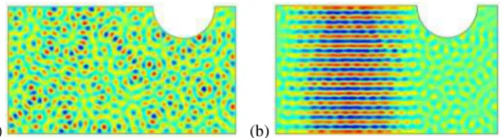
high frequencies). This hypothesis can be heuristically understood within the geometrical limit of rays at high frequency. Indeed, for ergodic enclosures the chaotic dynamics of rays leads to modelling eigenfields as a superposition of plane waves with fixed wavenumber but random directions and phases (an example of an ergodic mode in a 2D chaotic cavity is shown Fig. 1a).
(a) (b)
Fig. 1: Two modes of a Sinai-like 2D cavity with Dirichlet boundary conditions: (a) an ergodic mode, (b) a bouncing-ball mode. Such a semiclassical analysis also leads to statistical predictions about the sequence of eigenfrequencies. The salient feature of this approach lies in the fact that, whatever the specific details of a chaotic cavity, its spectral fluctuations exhibit a universal behavior. This universality underlies the relevance of a global approach consisting in generating artificial spectra through the eigenvalues of large random matrices. This is precisely the concerns of Random Matrix Theory (RMT). The intimate connection between semiclassics and RMT has been anticipated by the famous Bohigas-Giannoni-Schmit conjecture [21] and verified many times in various contexts [6]. Within the framework of RMT, the Gaussian randomness of modes is directly obtained from the statistical features of eigenvectors of random matrices. Deviations from universal behavior are an important issue and are equally manifested in the field distributions of modes and in the fluctuations of the corresponding spectra.
As an illustration in a 2D chaotic cavity, a mode showing a clear deviation with respect to the ergodic universal behavior of the field is depicted in Fig. 1b. This mode is often referred as a bouncing-ball mode since it is built on ray trajectories bouncing back and forth between parallel walls. The properties of statistical homogeneity and isotropy are therefore not fulfilled for such modes. Due to their regular occurrence in the spectrum, bouncing-ball modes contribute to significant spectral fluctuations on a large frequency range (compared to the mean spacing between adjacent eigenfrequencies) as will be illustrated in Section V.
In a 3D parallelepipedic cavity with defocusing parts of the boundary, chaotic ray motion is expected. However, regularity of modes may subsist due to families of ray trajectories which bounce in a plane parallel to a pair of walls. Indeed, the so-called tangential modes [22] constitute the most important family of regular modes whose wave vector is quantized in such planes. In the following sections, we will show how to reduce their spatial and spectral influence and thus obtain ideal homogeneity and isotropy for almost all modes of a chaotic RC.
Drawing inspiration from the 2D chaotic cavity of Fig. 1 [23], we studied three parallelepipedic cavities of dimensions W = 0.785 m along (Ox), L = 0.985 m along (Oy) and H = 0.995 m along (Oz), provided with metallic hemispheres or spherical caps on their walls (Fig. 2). Hemispheres and caps
positions are chosen to avoid any geometrical symmetry. Hemispheres have a radius of 15 cm and caps of 45 cm and 50 cm. The highest penetration depth of the caps within the cavity is of 15 cm. The first cavity, Cavity_1 (Fig. 2a), is directly inspired from the 2D cavity of Fig. 1. It comprises a hemisphere fixed on its wall at z = H. For the second cavity, Cavity_2 (Fig. 2b), a second hemisphere has been added on the plane y = 0. The third cavity, Cavity_3 (Fig. 2c), comprises two caps on the planes z = H and y = L, as well as one hemisphere on the x = W plane. The choice of the geometric modifications from Cavity_1 to Cavity_3 will be discussed later on while explaining how non-ergodic modes can appear within these cavities. In these three cavities, the stirring process, beyond the scope of this paper, can be insured by moving one (or two) hemisphere(s) on the related wall.
To assess the respective performances of the chaotic cavities, the distributions of the three electric field components are examined for each of them and compared to the case of a parallelepipedic cavity equipped with a mode stirrer (Fig. 2d). The shape and location of the latter is conform to an industrial RC, except a global scaling factor. As for the three other cavities, the cavity with the mode stirrer is studied in a fixed configuration i. e. for a single position of the stirrer.
(a) Cavity_1: with one hemisphere (b) Cavity_2: with two hemispheres
(c) Cavity_3: with 2 caps & 1 hemisphere (d) Cavity_4: with a mode stirrer Fig. 2: Cavity shapes and 3D grids for field values extraction. The first 450 modes of each cavity are obtained by using HFSS software. The corresponding resonant frequencies vary between 214 MHz and about 1.28 GHz. To study the field distributions, the values of the three electric field components are recorded for each mode at 1001 points within the cavity volume. As shown in Fig. 2, these points are taken on a 3D grid sampling a reduced volume in the cavities. The distance between two adjacent lines as well as between the limits of the
volume of use and the cavity is of 50 mm. For each eigenmode, the mean of the square electric field amplitude on the grid points is normalized to one.
In Section III, we focus on the electric field properties. Using simulation results, we first consider the distribution of each field component and determine if a Gaussian law is followed. We then examine the isotropy of the fields associated to the cavity resonances through a rotation of the orthonormal basis. In Section IV, we propose to use the standard deviations of the electromagnetic field components to build an indicator of the field isotropy. In Section V, we show how the conclusions of the previous sections (related to spatial statistics) can also be established through the spectral statistics of the cavities: the more complex the geometry, the more reduced the deviations from the universal behavior.
III. FIELD DISTRIBUTIONS
We first examine the distribution of the three electric field components for each eigenmode. The orthonormal basis is defined according to the cavity edges as reported in Fig. 2. In a well-operating reverberation chamber, as for the ergodic modes of a chaotic cavity, a normal distribution is expected for each field component.
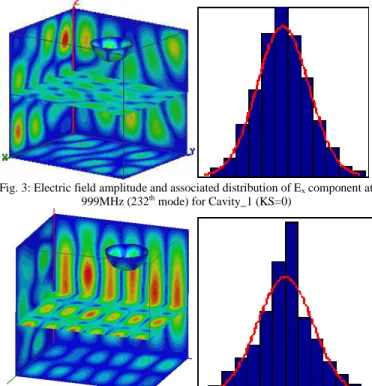
Let us consider as an example the mode at 999MHz (232th mode) for the cavity with one hemisphere (Fig. 3). The mapping of the electric field amplitude shows, while comparing to the parallelepipedic cavity, that the disturbance associated to the hemisphere is global within the cavity, and not located in the vicinity of the hemisphere. From the 1001 values of the electric field components extracted along the 3D grid, we build the distribution of amplitude of each field component. In Fig. 3 the numerically obtained histogram for Ex is succesfully compared to a normal distribution. To
quantify the agreement, the Kolmogorov-Smirnov (KS) test at 95% confidence is used. The result of the test is 0 if the histogram and the normal law match within the confidence interval and 1 otherwise. For the mode studied in Fig. 3, the answer is 0. Let us now consider the mode at 994MHz (230th mode) for the same cavity (Fig. 4). The regularity of the field mapping indicates that this mode corresponds to a tangential mode lying in xy plane. The associated histogram of Ex
confirms this observation as it is not fitted by a normal distribution: the answer of the KS test is 1 in this case.
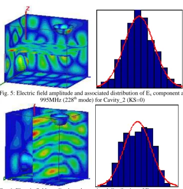
The insertion of a second hemisphere (Fig. 2b) aims to eliminate this kind of tangential modes. In the case of the 228th mode (995MHz) of the cavity with two hemispheres, a normal distribution of Ex is obtained (Fig. 5). Tangential
modes are however still observed, as with the 174th mode corresponding to a reflection between the bottom and the top of the cavity (Fig. 6). The replacement of hemispheres by caps (Fig. 2c) in the third cavity allows a reduction of facing plane surfaces. The suppression of the reflection between the two vertical walls orthogonal to x-axis is however insured by inserting a hemisphere instead of a cap for stirring purpose, this hemisphere being intended to move along its related wall while using this RC. We will see in the following that, according to these design principles of a chaotic cavity, the
field properties are progressively improved through the modifications from Cavity_1 to Cavity_3.
The KS test is performed with the first 450 eigenmodes of all cavities. The results obtained for the Ex components of the
eigenmodes are given in Fig. 7(a)-(d) for the four cavities. The increase of the number of zero-answers due to hemispheres and caps insertion clearly appears. Moreover, the Gaussian character of the field improves with increasing frequency in the four cavities: whereas the Ex components of
a large majority of the first modes are not normally distributed, the opposite conclusion can be drawn after the 120th mode. The same tests performed on Ey and Ez
components of the modes confirm these findings.
The results obtained for the three electric field components are summarized in Table I. The normal law is largely followed in Cavity_3 with a success ratio of the KS test above 89% for each electric field component when considering all modes. The lowest ratios are related to the cavity with one single hemisphere. The results obtained for the two other cavities are similar, with a mean success ratio over the three components of 84.4% with two hemispheres and 87.3% with a stirrer; however, the cavity with a stirrer presents a higher heterogeneity of the results associated to each component, the success ratio varying between 81% and 90% in this case against a variation between 84% and 88% with the two hemispheres.
As in all cavities, most of the first modes do not pass the test and the success ratio increases with the mode order, the success ratio has been calculated by excluding the first 30 modes (in brackets in Table I). All the success ratios are then increased. Thus, in Cavity_3, the success ratio of the KS test exceeds 92% after eliminating the first 30 modes.
Fig. 3: Electric field amplitude and associated distribution of Ex component at
999MHz (232th mode) for Cavity_1 (KS=0)
Fig. 4: Electric field amplitude and associated distribution of Ex component at
Fig. 5: Electric field amplitude and associated distribution of Ex component at
995MHz (228th mode) for Cavity_2 (KS=0)
Fig. 6: Electric field amplitude and associated distribution of Ex component at
913MHz (174th mode) for Cavity_2 (KS=1)
(a)
(b)
(c)
(d)
Fig. 7: KS test for Ex component of each mode (mode order in abscisse)
obtained with (a) Cavity 1, (b) Cavity_2, (c) Cavity_3, (d) Cavity_4.
TABLEI KS_95%= 0 KS_95% = 1 Cavity_1 Ex 80.89 (84.52) 19.11 (15.48) Ey 82.44 (85.95) 17.56 (14.05) Ez 81.33 (85) 18.67 (15) Cavity_2 Ex 84.44 (88.81) 15.56 (11.19) Ey 87.33 (92.14) 12.67 (7.86) Ez 87.78 (92.62) 12.22 (7.38) Cavity_3 Ex 89.56 (93.81) 10.44 (6.19) Ey 90.22 (94.52) 9.78 (5.48) Ez 89.11 (92.86) 10.89 (7.14) Cavity_4 Ex 90.22 (93.81) 9.78 (6.19) Ey 81.33 (84.52) 18.67 (15.48) Ez 89.33 (93.57) 10.67 (6.43)
Results (%) of the KS test performed on the distribution of the three field components for the 450 resonant modes of cavities, and in brackets while excluding the first 30 modes.
As, for an ergodic mode, the three field components are normally distributed, we now define a global homogeneity indicator of the three components properties. It takes the value of 0 if each component follows a normal distribution, and 1 if at least one of the components does not follow a normal distribution.
(a)
(b)
(c)
(d)
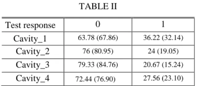
Fig. 8: Global homogeneity test for each mode (mode order in abscisse) obtained with (a) Cavity 1, (b) Cavity_2, (c) Cavity_3, (d) Cavity_4. In the four cavities, many of the modes follow a normal distribution (Fig. 8(a)-(d)). Table II summarizes the results of this global test for all the modes in all cavities. It clearly indicates that the insertions of a second hemisphere then caps significantly increase the number of modes with three normally distributed components. Once again, the best homogeneity is obtained for the cavity with two caps and a
hemisphere: 79% of the modes have their three components following a normal distribution, and the success ratio reaches 84% after eliminating the first 30 modes. According to this test, the homogeneity obtained with two hemispheres is better than with the stirrer (with a success ratio of 76% against 72%). As expected, the cavity with one single hemisphere leads to the lowest success ratio, with a value of 64%.
The success ratios obtained while excluding the first 30 modes are indicated in brackets in Table II. All the success ratios are increased, but the conclusions on the comparison between the four cavities remains unchanged.
TABLE II Test response 0 1 Cavity_1 63.78 (67.86) 36.22 (32.14) Cavity_2 76 (80.95) 24 (19.05) Cavity_3 79.33 (84.76) 20.67 (15.24) Cavity_4 72.44 (76.90) 27.56 (23.10) Results (%) of the global homogeneity test performed on all modes, and in brackets by excluding the first 30 modes.
Besides homogeneity, the field is also required to be isotropic in a well-operating reverberation chamber. We recall that an ergodic field is also isotropic. The field isotropy will be studied in more details in the fourth part, but we will perform here a preliminary test on this property.
The test on the field isotropy is as follows. If the field is isotropic then it presents the same distribution regardless of the chosen orthonormal coordinate system. To verify this property, we modify the first chosen coordinate system of Fig. 2 by performing a rotation of r = 30° about the Ox axis, of
r = 20° about the Oy axis and of r = 60° about the Oz axis.
The already presented tests are then applied, for each eigenmode of the four cavities, to the three components related to this new basis. The results obtained for the global homogeneity indicator are presented in Fig. 9(a)-(d).
(a)
(b)
(c)
(d)
Fig. 9: Global homogeneity test, after basis rotation, for each mode, with (a) Cavity_1, (b) Cavity_2, (c) Cavity_3, (d) Cavity_4.
TABLE III Test response 0 1 Cavity_1 72.67 (77.62) 27.33 (22.38) Cavity_2 80.22 (85.48) 19.78 (14.52) Cavity_3 82.00 (87.86) 18.00 (12.14) Cavity_4 82.44 (86.67) 17.56 (13.33) Results (%) of the global homogeneity test, after basis rotation, for all modes,
and in brackets by excluding the first 30 modes.
As a consequence of the use of a coordinate system independent of the geometry particularities, an increase of the rate of zero answers to the global homogeneity test is observed for the four cavities (Table III) either by considering all modes or by excluding the first 30 ones. For all modes, this increase is of 8.89% in Cavity_1, 4.22% in Cavity_2, 2.67% in Cavity_3 and 10% in Cavity_4. These changes of the test answers indicate that the associated modes are not ergodic as their field distributions are sensitive to the chosen projection basis. As the test response is the least sensitive to the coordinate system for Cavity_3, we can suppose that a better isotropy is attained in this cavity. This will be confirmed using another test.
The modes whose three components are normally distributed in both coordinate systems, as expected for Gaussian ergodic modes, are presented in Fig. 10(a)-(d). For each mode, if the global homogeneity test takes the value 0 in both coordinate systems, then 0 is indicated, else 1 is associated to this mode. The zero answer is obtained for 56% of all modes with one hemisphere, 70% with two hemispheres, 74% with two caps and one hemisphere, and 68% with the stirrer (see Table IV). As with the previous indicator, we can conclude that the best performances are obtained with Cavity_3 then Cavity_2.
As already noticed, the field statistical properties improve with increasing frequency for all cavities. The percentage of normally distributed modes in both bases increases for the four cavities when omitting the first 30, 50 and 100 modes (Table IV). Thus, from the 101th mode, 90% of the modes of Cavity_3 pass the test in both coordinate systems. It has to be noticed that the third cavity always presents the best performances and the first cavity the worst either considering all the modes or after eliminating the first ones.
The very first modes of all cavities do not pass the homogeneity test. The first zero answer appears respectively at the 55th mode in Cavity_1, 40th mode for Cavity_2, 33th mode for Cavity_3 and 20th mode for Cavity_4, but the zero answers are at the lowest frequencies isolated and the one value remains majoritary up to about one hundred modes. At higher frequencies, the one values appear isolated: the last two successive one answers occur at rank 342-343 for Cavity_1,
273-274 for Cavity_2, 151-152 for Cavity_3 and 263-264 for Cavity_4. Due to mode overlapping at high frequency, the presence of isolated non-homogeneous modes migh be less detrimental to the field uniformity than two consecutive non- homogeneous modes. The superiority of Cavity_3 is also observed for this aspect.
(a)
(b)
(c)
(d)
Fig. 10: Global homogeneity test in both bases for each mode of (a) Cavity_1, (b) Cavity_2, (c) Cavity_3, (d) Cavity_4.
TABLE IV All the
modes
From the
31th mode From the 51th mode From the 101th mode Cavity_1 56.44 60.48 63.5 70.29 Cavity_2 69.56 74.52 77 85.14 Cavity_3 74.44 79.29 82.75 90.29 Cavity_4 68.00 72.38 75.25 82.28
Percentage of modes presenting normal distributions in both bases
To further investigate the field isotropy, the standard deviations of the three field components of each mode will now be examined.
IV. STANDARD DEVIATION AND FIELD ISOTROPY The field isotropy implies an equality of the standard deviations of each field component. Therefore, we examine here the standard deviations of the three electric field components for each eigenmode, and use the difference
between them as an indicator of the field istropy. The orthonormal basis as defined in Fig. 2 is chosen.
The standard deviations are calculated for each eigenmode from the component values at the 1001 sampling points, for each cavity. The mode dependence of the 3 standard deviations is depicted in Fig. 11 for the cavity with a hemisphere, and in Fig. 12 for the cavity with two caps and one hemisphere (the same analyses were also performed for the other two cavities).
Mode order
Fig. 11: Standard deviation of Ex, Ey and Ez for Cavity_1.
Fig. 12: Standard deviation of Ex, Ey and Ez for Cavity_3.
We notice a decrease of the standard deviations excursion when frequency increases for both cavities. Whatever the frequency, the standard deviation fluctuations are much smaller in Cavity_3. The value of 0.577 indicated in Figs. 11 and 12 corresponds to an ideal Gaussian mode whose three components have a zero mean and identical standard deviations. It is expected in a chaotic cavity that the standard deviations fluctuate around this value. This behavior is observed with Cavity_3.
The mean values of the standard variations of each components are given in Table V; the first 30 modes have been excluded to the mean calculation as we already showed that the first modes are not homogeneous. The obtained mean values are compared (into brackets) to the ideal 0.577 value. It appears that the smallest differences are obtained with
Cavity_3 then Cavity_2, whereas Cavity_1 presents the largest ones. TABLE V Std. deviations and Ex Ey Ez Cavity_1 (0.04) 0.537 (0.033) 0.544 (0.047) 0.530 0.418 Cavity_2 0.549 (0.028) 0.564 (0.013) 0.556 (0.021) 0.289 Cavity_3 0.563 (0.014) 0.572 (0.005) 0.571 (0.006) 0.177 Cavity_4 0.567 (0.01) 0.539 (0.038) 0.545 (0.032) 0.328 Means of the standard deviations of each component and of from the 31th
mode. In brackets, the difference between 0.577 and each mean standard deviation.
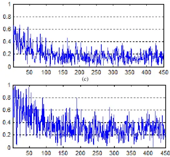
Thus, in the ideal case of an isotropic field, the standard deviations of the three electric field components are equal. To evaluate the isotropy of the modes, we propose the indicator
defined in Eq. 2. Its value, comprised between 0 and 1,
decreases when the three standard deviations become similar.
is equal to 1 when one field component vanishes whereas,
in the ideal isotropic case, it is vanishing.
(2)
(a)
(b)
(c)
(d)
Fig. 13: versus frequency of each mode (mode order in absisse) for (a) Cavity_1, (b) Cavity_2, (c) Cavity_3, (d) Cavity_4.
Fig. 13(a)-(d) indicates highly varies with the mode order. However this indicator globally decreases with the frequency in all cavities, with a stabilization of its mean and standard deviation around the 150th mode. In the whole frequency band, we notice that the lowest mean and maximal values of are obtained with Cavity_3. The mean values of
, calculated for each cavity from its 31th mode, are given in
Table V. The lowest mean values are obtained with Cavity_3 then Cavity_2, indicating an improvement of the field isotropy compared to the classical RC equipped with a mode stirrer.
Fig. 14: Evolution of the spectral fluctuations. Fluctuating part of the counting functions, N-Nav, for (a) Cavity_1, (b) Cavity_2, (c) Cavity_3 and (d)
Cavity_4 (continuous lines) ; NTgM is the contribution of the tangential modes
(red dotted line). The value of the standard deviation of N-Nav is indicated in
the inset.
x y z
x y z
z y x z y x , , min , , max , , min , , max -4 0 4 8 12 (a) σ=3.16 N-Nav NTgM -8 -4 0 4 8 (b) σ=2.70 -4 -2 0 2 4 (c) σ=1.34 -8 -4 0 4 8 0.5 0.6 0.7 0.8 0.9 1 1.1 1.2 frequency in GHz (d) σ=2.80V. SPECTRAL FLUCTUATIONS
RMT has introduced various statistical tools to analyze spectral fluctuations of chaotic cavities [6]. We use here the simplest one: the fluctuations of the counting function N(f). The latter gives the number of resonant modes up to the frequency f. Its smooth part Nav is related to the geometry of
the cavity through the Weyl's law [24]. In Fig. 14(a)-(c) the fluctuating part of the counting functions, N-Nav, respectively
associated with the 3 chaotic cavities is shown within the frequency range [0.4 GHz, 1.28 GHz]. For Cavity_1, with only 1 hemisphere, the deviations from RMT predictions concerning these fluctuations are important, thus indicating the significant presence of non-ergodic modes in the spectrum. Indeed, in spite of the defocusing part of the boundary, the cavity still possesses parallel walls and remains close to a parallelepipedic room. In such a cavity, many modes are reminiscent of the modes of a regular one for which ergodic features are not expected. The most important family of regular modes consists of tangential modes (TgM) which, in the parallelepipedic cavity, have a single null wave vector component. The non-zero components are quantized in the planes parallel to the walls of the cavity. The counting function for TgM perpendicular to each axis can be obtained through a procedure introduced in Ref. [19] and has recently been extended by Gros et al. [25] to the case of RCs. In Fig. 14, the red dotted curve corresponds to the contribution of TgM to N-Nav. Note that the amplitudes of the fluctuations are
progressively reduced from Cavity_1 to Cavity_3 due to the corresponding suppression of TgM. In Cavity_3, the remaining fluctuations are much closer to the amplitude predicted by RMT. As in the previous sections, the comparison is extended to Cavity_4 (Fig. 14(d)) which, here again, exhibits a behavior intermediate between Cavity_1 and Cavity_2. And this is particularly well illustrated by evaluating the standard deviation of N-Nav as shown in the
inset for each cavity.
VI. CONCLUSION
As most resonant modes in chaotic cavities present homogeneous and isotropic fields, we drew inspiration from studies developped in the field of wave chaos to propose three simple geometric modification of a parallelipedic cavity with the aim of following the requirements for well-operating RCs. Using simulation results, comparisons between these three chaotic cavities and a classical RC equipped with a mode stirrer have been performed. In a first stage, we demonstrated that the ratio of field components of modes following a normal distribution is, for two chaotic cavities, higher than for the classical RC, and that this ratio grows with increasing frequency. The field isotropy was also discussed from two different points of view. First, the invariance of the field statistical properties with respect to the orthonormal basis has been tested. Then, the analysis of the standard deviations of the three components and, for each mode, of their dispersions, confirmed the same trend. In complete accordance with these findings in the spatial domain, we also performed a comparison in the spectral domain. We showed how the
modifications of the chaotic cavities allow a significant reduction of the role of regular modes on the spectral fluctuations: by reducing the amount of facing parallel surfaces in the chaotic cavities, the spectral fluctuations become closer to those expected from RMT predictions.
An obvious conclusion from the results presented in this paper is that facing parts of parallel walls should be eliminated from any RC where ergodicity of modes is wanted. The very simple cavity modifications we propose, consisting of inserting metallic hemispheres or caps on the cavity walls, permit a significant improvement of the field statistical properties. The stirring process is not addressed in this paper but the adaptation of these new cavity shapes to mechanically stirred reverberation chambers could be performed in two ways. The first one would consist in improving a classical RC equipped with a stirrer by inserting metallic caps on its walls. In the second one, the chaotic cavity itself could be used as an RC and one hemisphere could be used as a mode-stirrer by moving it on the cavity wall. In both approaches, it is expected that the spectral overlap of homogeneous and isotropic modes will lead to better statistical field properties than when the modes do not individually meet the required statistical properties. It would result in the improvement of the reverberation chambers operation especially in the weak overlap regime, with a potential decrease of their LUF.
REFERENCES
[1] P.-S. Kildal, K. Rosengren, J. Byun, J. Lee, “Definition of effective diversity gain and how to measure it in a reverberation chamber”, Microwave and Optical Technology Letters, vol. 34, no. 1, pp. 56-59, July 2002.
[2] Larry K. Warne et al., “Statistical Properties of Linear Antenna Impedance
in an Electrically Large Cavity”, IEEE Trans. Antennas and
Propagation, vol. 51, no. 5, pp. 978-992, May 2003.
[3] M. O. Hatfield, M. B. Slocum, E. A. Godfrey, and G. J. Freyer,
“Investigations to extend the lower frequency limit of reverberation chamber,” in Proc. IEEE Int. Symp. Electromagn. Compat., Denver, CO,
1998, vol. 1, pp. 20–23.
[4] D. A. Hill, “Plane wave integral representation for fields in reverberation
chambers”, IEEE Trans. Electromag. Compat., vol. 40, no. 3, pp.
209-217, Aug. 1998.
[5] A. K. Mitra and T. F. Trost, “Statistical Simulations and Measurements Inside a Microwave Reverberation Chamber”, in Proc. IEEE/EMC Symposium, Austin, 1997, pp. 48-53.
[6] H.–J. Stöckman, Quantum Chaos: an introduction, Cambridge University Press, 1999.
[7] O. Legrand, F. Mortessagne, “Wave Chaos for the Helmholtz Equation” in New Directions in Linear Acoustics and Vibration: Quantum Chaos, Random Matrix Theory, and Complexity, Cambridge University Press, 2010.
[8] M.V. Berry, “Semiclassical mechanics of Regular and Irregular Motion”, in Chaotic Behaviour of Deterministic Systems, edited by R.H.G. Helleman and G. Ioss, Les Houches 82, Session XXXVI (North-Holland, Amsterdam, 1983).
[9] L. R. Arnaut, “Operation of electromagnetic reverberation chambers with
wave diffractors at relatively low frequencies,” IEEE Trans.
Electromagn. Compat., vol. 43, no. 4, pp. 635–653, Nov. 2001. [10] Andrea Cozza, “The Role of Losses in the Definition of the Overmoded
Condition for Reverberation Chambers and Their Statistics”, IEEE Trans. Electromagn. Compat., vol. 53, no. 2, pp. 296-307, May 2011. [11] D.I. Wu, D.C. Chang, “The effect of an electrically large stirrer in a
mode-stirred chamber”, IEEE Trans. Electromag. Compat., vol. 31, no. 2, pp. 164-169, May 1989.
[12] L. R. Arnaut, ”Limit Distributions for Imperfect Electromagnetic
Reverberation”, IEEE Trans. Electromag. Compat., vol. 45, no. 2, pp.
[13] C. Bruns, R. Vahldieck, “A Closer Look at Reverberation Chambers—3-D Simulation and Experimental Verification”, IEEE Trans. Electromag. Compat., vol. 47, no. 3, pp. 612-62, Aug. 2005.
[14] V. Galdi, I. M. Pinto, and L. B. Felsen, “Wave Propagation in
Ray-Chaotic Enclosures: Paradigms, Oddities and Examples”, IEEE Antennas and Propagation Magazine, vol. 47, no. 1, pp. 62-81, Feb. 2005.
[15] D. D. de Menezes, M. Jar e Silva, and F. M. de Aguiar, “Numerical experiments on quantum chaotic billiards”, Chaos, vol. 17, no. 2, May 2007.
[16] J. Barthélemy, O. Legrand, F. Mortessagne, “Complete S-matrix in a microwave cavity at room temperature”, Phys. Rev E, vol. 71, Jan. 2005. [17] S. Deus, P. M. Koch, and L. Sirko, “Statistical properties of the
eigenfrequency distribution of the three-dimensional microwave
cavities”, Phys.Rev. E, vol. 52, no. 1, pp. 1146–1155, Jul. 1995.
[18] U. Dörr, H. J. Stöckmann, M. Barth, and U. Kuhl, “Scarred and chaotic field distributions in a three-dimensional Sinai-microwave resonator”, Phys. Rev. Lett., vol. 80, no. 5, pp. 1030–1033, Feb. 1998.
[19] C. Dembowski, B. Dietz, H.-D. Gräf, A. Heine, T. Papenbrock, A.
Richter, and C. Richter, “Experimental Test of a Trace Formula for a
Chaotic Three-Dimensional Microwave Cavity”, Phys. Rev. Lett., vol. 89, no. 6, Aug. 2002.
[20] M. V. Berry, “Regular and irregular semiclassical wave functions”, J.Phys.A, vol. 10, no. 12, Dec. 1977.
[21] O. Bohigas, M. Giannoni, C. Schmit, “Characterization of chaotic quantum spectra and universality of level fluctuation laws”, Phys. Rev. Lett., vol. 52, no. 1, pp. 1–4, 1984.
[22] H. Kuttruff, Room acoustics, Taylor & Francis, 2000.
[23] R. A. Méndez-Sànchez, U. Kuhl, M. Barth, C. H. Lewenkopf, and H.-J.
Stöckmann, “Distribution of Reflection Coefficients in Absorbing Chaotic Microwave Cavities”, Phys. Rev. Lett., vol. 91, no. 17, Oct.
2003.
[24] H. Alt, C. Dembowski, H. Gräf, R. Hofferbert, “Wave dynamical chaos in a superconducting three-dimensional sinai billiard”, Phys. Rev. Lett. vol. 79, no. 6, pp. 1026-1029, Aug. 1997.
[25] J.-B. Gros, O. Legrand, F. Mortessagne, E. Richalot and K. Selemani,
“Universal behaviour of wave chaos based electromagnetic
reverberation chamber”, (submitted to Wave Motion, http://hal.archives-ouvertes.fr/hal-00800526).