The Performance of RAMS in Representing the
Convective Boundary Layer Structure in a Very
Steep Valley
STEPHAN F.J. DE WEKKERa,b,c,∗, D.G. STEYNa, J.D. FASTc, M.W. ROTACHd and S. ZHONGe
aThe University of British Columbia, Vancouver, BC, Canada;bPaul Scherrer Institute, Villigen,
Switzerland;cPacific Northwest National Laboratory, Richland, WA, U.S.A.;dSwiss Federal Office of Meteorology and Climatology, MeteoSwiss, Zurich, Switzerland;eGeosciences Department, University of Houston, Houston, TX, U.S.A.
Received 23 May 2003; accepted in revised form 24 January 2004
Abstract. Data from a comprehensive field study in the Riviera Valley of Southern Switzerland are
used to investigate convective boundary layer structure in a steep valley and to evaluate wind and temperature fields, convective boundary layer height, and surface sensible heat fluxes as predicted by the mesoscale model RAMS. Current parameterizations of surface and boundary layer processes in RAMS, as well as in other mesoscale models, are based on scaling laws strictly valid only for flat topography and uniform land cover. Model evaluation is required to investigate whether this limits the applicability of RAMS in steep, inhomogeneous terrain. One clear-sky day with light synoptic winds is selected from the field study. Observed temperature structure across and along the valley is nearly homogeneous while wind structure is complex with a wind speed maximum on one side of the valley. Upvalley flows are not purely thermally driven and mechanical effects near the valley entrance also affect the wind structure. RAMS captured many of the observed boundary layer characteristics within the steep valley. The wind field, temperature structure, and convective boundary layer height in the valley are qualitatively simulated by RAMS, but the horizontal temperature structure across and along the valley is less homogeneous in the model than in the observations. The model reproduced the observed net radiation, except around sunset and sunrise when RAMS does not take into account the shadows cast by the surrounding topography. The observed sensible heat fluxes fall within the range of simulated values at grid points surrounding the measurement sites. Some of the scatter between observed and simulated turbulent sensible heat fluxes are due to sub-grid scale effects related to local topography.
Key words: convective boundary layer structure, model evaluation, RAMS, thermally driven flow,
always present and the interaction between regional and local flows often results in complex flow patterns. The presence of cross-valley flows (blowing from one sidewall to the other) can also make the boundary layer structure more complicated and variable.
Simultaneous observations of the vertical wind- and temperature structure in a valley led to a conceptual model of the temporal evolution of the convective boundary layer (CBL) in deep valleys [2]. The role of slope flows in redistributing energy gained at the surface over the entire valley atmosphere plays an important role in this conceptual model. Also, the compensatory sinking motions that are produced over the valley center related to the withdrawal of mass by upslope flows, are a key aspect. Because the conceptual model is two-dimensional, the role of valley flows is not considered.
The three-dimensional spatial structure of wind and temperature including the CBL height along and across a valley has not been given much attention in previous research. In many studies, such as those where mass budgets are calculated, it is assumed that cross-valley temperature- and wind structure is homogeneous and that the along-valley structure is simple, with monotonically increasing/decreasing or constant flow speeds along the valley [3]. Similarly, little is known about turbu-lent energy exchange in valleys despite the well-known fact that turbuturbu-lent sensible heat input from the valley surface is crucial for the evolution of wind systems and boundary layers in valleys (e.g., [1]).
In this paper, surface and airborne data from the MAP-Riviera field study [4] and a mesoscale numerical model are used to study the spatial and temporal struc-ture of the wind- and temperastruc-ture field, the CBL height, and the surface sensible heat flux in a deep and narrow valley. Even though the field study provided a large data set, spatial information at the surface remains limited and aircraft meas-urements aloft are only available for limited periods. A numerical model could provide the information to examine the full diurnal evolution and spatial struc-ture of the valley atmosphere. Also, in order to use the results of the numerical simulations as a tool to better understand the CBL structure, a proper evaluation
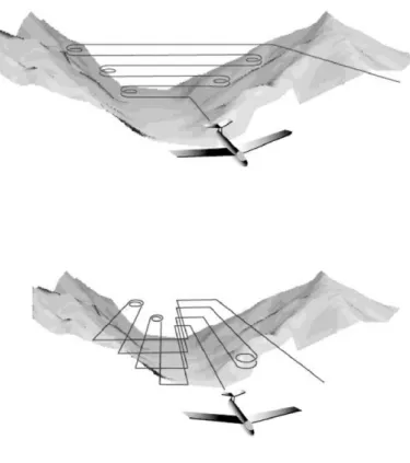
Figure 1. (a) Topography of the Riviera Valley and surroundings. Contour lines are drawn every 400 m. Terrain above 2000 m asl is shaded. The dashed lines depict the cross-valley and along-valley cross sections. The main valley site, site A1, (46.26◦N, 9.01◦E, 250 m asl) is located near Claro in the valley center. The inner square represents the area in (b). (b) Zoomed-in part of (a) with the location of the surface turbulence stations. See Table I for details. The scale of the axes corresponds to that in (a). Contour lines are drawn every 100 m. Data from Bundesamt für Landestopographie, permission # JD002102.
with observational data is required. Since operational models are expected to be applied at resolutions of a few kilometers or smaller, an evaluation of mesoscale models at such a high resolution is needed. In this way, weaknesses and strengths of the mesoscale models can possibly be identified. The MAP-Riviera field study provides both an extensive data set for model evaluation at a grid spacing of less than one kilometer in complex terrain, and allows detailed investigation of CBL structure. Such a modeling study has not been performed before in a complex terrain as steep as in the Riviera Valley.
2. Data and Numerical Model Setup 2.1. DATA
A comprehensive boundary-layer field study, described by Rotach et al. [4], was carried out from August to October 1999 in the Riviera Valley of southern Switzer-land. This field study was part of the larger scale Mesoscale Alpine Programme (MAP) field project [5], and is referred to as the MAP-Riviera field study.
A map of the topography in the area is shown in Figure 1a. The Riviera Valley is located in the southern Alps, about 100 km north of Milan, between the towns of Bellinzona in the south (240 m asl) and Biasca in the north (300 m asl). The Riviera Valley is a U-shaped valley with several tributary valleys. Its orientation is from
Figure 2. Flight patterns in the cross-valley (top) and along-valley (bottom) directions.
southeast to northwest (155◦–335◦). The valley is narrow and steep with a valley floor width of 1.5 km, a depth between 2 and 2.5 km, and slope angles of roughly 30◦on the eastern slope and 35◦on the western slope. The valley floor has a length of about 15 km, and an average slope angle of less than 0.5◦. The highest peak is at 2727 m asl. The topography of this valley is typical of the southern European Alps. The valley floor consists of agricultural land and a number of small villages. A highway, railroad, and river run along the valley. The slopes are covered mainly with deciduous trees up to 1000 m asl, with conifers above. The treeline is at about 1800 m asl with areas of bare ground and short grass at higher elevations.
During eight ‘flight days’, an instrumented light aircraft operated by MetAir [6] flew specified patterns inside the valley. The flight days cover a variety of weather situations, from overcast days where mechanically driven turbulence is expected to play a dominant role to dry, cloudless, convective days. The present study uses data from the 25 August 1999 (Julian day 237) flight day, which had dry, convective weather. Astronomical sunrise was at 0435 UTC and sunset was at 1817 UTC.
On 25 August 1999, a high-pressure ridge extending from North Africa to Scandinavia influenced the weather in the investigation area. Synoptic flows were
Table I. Site identification, location, measurement height, and some surface characteristics for the ten surface stations measuring turbulence.
Site Location Measurement Surface characteristics lat (◦N), lon (◦E), height (m agl)
elev (m asl) A1 46.2572, 9.0131, 250 3.56 Valley floor; mixed agriculture A2 46.2500, 9.0153, 250 1.15 Valley floor; mixed agriculture B 46.2647, 9.0311, 760 23.78 Slope; forest
(mean height of trees∼ 15 m) C 46.2494, 9.0056, 340 6.33 Slope; vineyard
D 46.2467, 9.0269, 256 2.62 Valley floor; mixed agriculture E1 46.2667, 9.0372, 1060 12.70 Slope; meadow E2 46.2706, 9.0364, 1030 22.68 Slope; forest
(mean height of trees∼ 13 m) F1 46.2700, 9.0553, 1750 6.30 Slope; sparse vegetation F2 46.2728, 9.0608, 2110 1.30 Slope; shrub
(∼75 m bleow ridgeline) G 46.2742, 9.0317, 870 5.25 Slope; forest
(bridge over small tributary valley)
weak to moderate (15 m s−1 at 500 hPa) from northwesterly directions (∼300◦). The combination of northerly synoptic flows with southerly valley flows is known as inverna in this region and is a common wind pattern in the southern Alps [7]. The satellite image for 1419 UTC on this day (not shown) shows cloudless conditions over the Alps and a major part of central Europe.
The data set for this case study includes a set of surface turbulent flux data obtained at ten different measurement sites on the valley floor and sidewalls. The measurement sites exhibit a large heterogeneity in slope and surface characteristics. Details of the measurement sites are provided in Table I; the locations are shown in Figure 1b. All slope sites, except for site C, were located on the west-facing slope. Small-aperture scintillometers were installed at A2 and D measuring over a path length of about 100 m. Sonic anemometers were installed at all the sites except for site A2. Measurements of turbulent sensible heat and momentum fluxes were made at all sites. At a few sites, latent heat fluxes were also measured. In the present study only sensible heat flux measurements will be presented. At several sites, radiation measurements were also taken. Radiosondes were launched on 25 August 1999 at 0739, 0915, 1208, 1508, and 1800 UTC. The aircraft operated
between 0649 and 0942 UTC in the morning and between 1112 and 1541 UTC in the afternoon. In the morning, three across- and one along-valley flights were made. In the afternoon, three across- and two along-valley flights were made. A schematic of the flight patterns is depicted in Figure 2. Data from selected flight legs will be used in the current paper. Accuracy of rawinsonde and aircraft data is on the order of 0.1–0.5 K for temperature and 0.5 m s−1 for wind speed. Specific information about the instrumentation can be found in Rotach et al. [4].
2.2. NUMERICAL MODEL SETUP
The mesoscale numerical model used is the Regional Atmospheric Modeling Sys-tem (RAMS) [8, 9], in which land-surface processes are represented by the Land Ecosystem Atmosphere Feedback Model, version 2 (LEAF-2) [10]. The simula-tions use two-way interactive, nested grids. The model domain consists of four nested grids with horizontal grid spacing of 9, 3, 1, and 0.333 km, respectively. The outermost grid covers central Europe including the Alps while the innermost grid is the area shown in Figure 1a. All four grids have 38 vertical levels, with a grid spacing from 70 m near the surface that gradually increases to 1000 m near the model top at about 16 km. Due to vertical grid staggering, the first model level for all variables except for vertical velocity is at about 35 m. Simulations in which the vertical grid spacing was set to smaller values became numerically unstable. Thirteen soil nodes were used to a depth of 0.9 m below the surface. Details of the four grids used in the simulations are given in Table II.
The simulations cover 36 h from 1200 UTC 24 August to 0000 UTC 26 August 1999. The five outermost lateral boundary points in the largest domain were nudged using an implementation of the Davies [11] scheme toward ECMWF objective analysis fields at 6-h intervals and rawinsonde data to allow changes in large-scale conditions to influence the model simulations. Nudging towards objective analysis fields was only applied to the outermost grid; no interior nudging was applied.
The land use and topography in grids 1, 2, and 3 were derived from 30 arcsecond (∼ 1 km) resolution data from the United States Geological Survey (USGS) data set. The USGS land use data set is based on 1 km resolution Advanced Very High Resolution Radiometer (AVHRR) data spanning April 1992 through March 1993.
For the innermost grid (with 333 m grid spacing), topography and land use were obtained from a 100 m resolution Swiss topography and land use (BFS, [12]) data set. Land use types in the Riviera Valley from the 1 km USGS data set were found to give a poor representation of reality [13]. Thus, use of the high resolution Swiss BFS data set was deemed necessary. Most land use classes in the BFS data set did not match those in LEAF-2. Also, the BFS data set contains many more classes (69) than LEAF-2 (31). Therefore, land use classes from the BFS data set had to be cross-referenced to land use classes of LEAF-2. The BFS data set did not distinguish between needleleaf and broadleaf trees. By inspecting photographs and satellite-derived vegetation patterns in the Riviera Valley, the boundary between broadleaf and needleleaf trees was put at 1000 m asl with only needleleaf above and broadleaf below that boundary.
Modeling studies have noted the importance of a correct soil moisture ini-tialization for simulating atmospheric processes in a numerical model [14, 15]. Soil moisture is often used inappropriately as a tuning parameter to obtain good agreement with atmospheric observations. Despite the fact that spatial variability of soil moisture in complex mountainous terrain can be important for boundary-layer processes, it is usually neglected or inadequately initialized because of a lack of data. Soil moisture measurements were taken at a few sites in the Riviera Valley but there is insufficient information about its spatial variability. To improve the soil moisture initialization for the present case study, soil moisture distribution for the innermost grid was obtained from a WaSiM simulation (Water balance Simulation Model, a hydrological model developed at ETH-Zürich [16]. The simulation was made in hourly time steps from 1 January 1999 through the initialization time of the RAMS simulation. The spatial resolution is 500× 500 m and the simulation was done for the two catchment areas covering the major part of the innermost grid. Soil moisture distribution in the Riviera Valley and adjacent sidewalls was rather inhomogeneous, with typical values around 0.31 m3m−3. These soil moisture val-ues compared well with observations of soil moisture at sites A1 and B in the valley (for details about soil moisture measurements, see [17]). At high elevations where bare soil is present, the soil moisture is considerably reduced in the model. Soil type in the simulations was set to loamy sand, which is the predominant soil type in the Riviera Valley [16] and has a saturated volumetric soil moisture of 0.41 m3m−3.
For the other grids, a constant volumetric soil moisture of 0.28 m3 m−3 was assumed. This value is more representative of the inner Alps which has a drier climate than the southern part of Switzerland covering the Riviera Valley (e.g., [18]). Sensitivity studies showed that the boundary-layer structure inside the Rivi-era Valley is not very sensitive to the specific value of the soil moisture in the outer
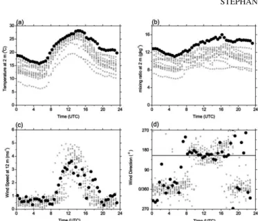
Figure 3. Temperature (a), mixing ratio (b), wind speed (c) and wind direction (d) at the surface (2 m for temperature and mixing ratio, 12 m for wind) at site A1 for all valley wind days during MAP-Riviera (open circles). The closed circles are the data for 25 August 1999. Upvalley wind direction is indicated by the horizontal black line in (d).
grids. Thus, the lack of information about soil moisture for these grids is not crucial to this study.
The turbulent exchange at the surface is determined with the so-called Louis scheme [8, 9] which is based on Monin–Obukhov similarity theory. The com-puted surface fluxes for the soil and vegetation must be averaged to provide the grid-averaged surface flux. These fluxes serve as the lower boundary for the sub-grid diffusion scheme for the atmosphere. For more detailed descriptions of the treatment of physics in RAMS, see [8, 9].
3. Results and Discussion
In the following sections, RAMS output is compared with surface meteorological data, radiosonde profiles, and aircraft measurements. CBL heights, which limit the vertical extent of turbulent mixing and are therefore an important parameter, for example, in air pollution studies, are determined from model output, and com-pared with observations. The turbulent sensible heat input from the valley surface provides the energy needed to drive the evolution of wind systems and boundary layers in valleys. Therefore, modeled and sensible heat fluxes are also compared.
3.1. TEMPORAL EVOLUTION OF SELECTED VARIABLES AT THE SURFACE
Andretta et al. [19] selected a set of so-called ‘valley wind days’ for the Riviera Valley from the 21 August to 16 October 1999 study period to facilitate their
in-Figure 4. Observed (filled circles) and modeled (open circles) net radiation (a) and temperat-ure (b) at site A1 on 25 August 1999.
vestigation of the near surface turbulent characteristics of the valley boundary layer. Valley wind days are characterized by a regular pattern of the diurnal evolution of the wind field [20, 21]. The criteria for the selection of valley wind days included a strong diurnal range of pressure gradient between two sites north and south of the Riviera Valley, weak synoptic flows and a large diurnal range of global radiation (fair weather days). These days cover about 20% of the entire measuring period. Figure 3 shows the diurnal course of temperature, mixing ratio, wind speed, and wind direction on valley wind days for site A1 in the center of the valley (see Figure 1b). The diurnal range on 25 August 1999, the case study in this paper, is highlighted in the figure with filled circles. It can be seen that 25 August 1999 was the warmest (up to 28◦C) and most humid (up to 16 g kg−1) of the valley wind days. Compared to all the other valley wind days in the field study, the thermal forcing of the boundary layer on this day is expected to be relatively large, making it a suitable day for the investigation of CBL structure in this valley. Wind direction shows an onset of upvalley flows at about 0800 UTC, about 3.5 h after sunrise (0435 UTC). Upvalley flows cease shortly after sunset (1817 UTC). Wind speed increases after the onset of the upvalley flow to about 4 m s−1 at around 1300 UTC and decreases (and becomes more variable) afterwards. The daytime wind is approximately aligned with the upvalley direction indicated by the horizontal solid black line at 155◦. The wind speed and direction on 25 August do not deviate significantly from the average behaviour.
Figure 4 shows the diurnal course of observed and modeled net radiation and temperature at site A1 in the valley center for 25 August 1999. The data are half-hourly averaged values while the model output represents instantaneous half-hourly val-ues. The temperature at the first model level at∼ 35 m was extrapolated downward to observation height using Monin–Obukhov similarity functions (e.g., [22]).
Net radiation is somewhat overestimated by the model in the early morning and late evening. Even though the mesoscale model takes into account the effect of slope steepness and orientation on the incoming shortwave radiation (following Kondratyev [23]) the model does not take into account the shadowing of a loca-tion by the surrounding topography. Colette and Street [24] recently modified the radiation code in a numerical model to account for the shadowing and found that
Figure 5. Horizontal wind vectors plotted as a function of time at site A1, as observed at 12 m agl (top panel) and modeled at 10 m agl (bottom panel) for 25 August 1999.
inversion-layer breakup in steep valleys was slightly retarded by shadowing. Some clouds were present in the afternoon, which explains the short-term reduction of the radiation values at around 1300 UTC. The agreement in the diurnal temperature range is good, as the model underestimates the minimum and maximum temperat-ure by only 1–2 K. The rate of increase in temperattemperat-ure after sunrise is particularly well simulated. This is important since the boundary-layer structure is examined in more detail later in this paper after approximately 0700 UTC and before 1500 UTC. The decrease in temperature in the early evening is somewhat underestimated by the model.
Figure 5 shows the observed and modeled horizontal wind vectors at site A1 as a function of time. The 10-m wind speed was obtained by extrapolating the wind speed downward from the first model level using Monin–Obukhov similarity functions. The model clearly shows upvalley flows with speeds that are generally somewhat weaker in the early afternoon and stronger in the late afternoon and evening than the observed wind speeds. Upvalley flows start about 2 h later in the model than in the observations at this particular location. Also, the upvalley flow in the model intensifies with time in the afternoon and evening, reaching a maximum at 1900 UTC, a feature that was not observed.
3.2. TEMPORAL EVOLUTION OF THE VALLEY ATMOSPHERE
3.2.1. Observed profiles of temperature, humidity, and wind
At 0739 UTC, an inversion from the previous night is present (Figure 6a) and light and variable winds are observed (Figure 7a). As was shown in Figures 3 and 5, surface observations show a change from downvalley to upvalley winds at about 0800 UTC. At 0915 UTC, a CBL is observed up to 650 m asl capped by a weak inversion (Figure 6c). The CBL grows only a few hundred meters between 0915 and 1208 UTC and reaches a height of around 800 m asl after that (Figures 6e, g).
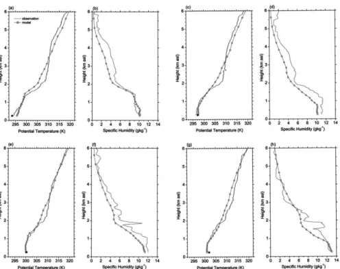
Figure 6. Vertical profiles of observed (solid lines) and modeled (circles) potential temperat-ure and specific humidity at site A1 on 25 August 1999 at 0739 (a, b), 0915 (c, d), 1208 (e, f), and 1508 UTC (g, h). Model output is for 0700 (a, b), 0900 (c, d), 1200 (e, f), and 1500 UTC (g, h). Surface potential temperatures measured at 1.5 m agl are indicated by black squares in (a, c, e, g). The approximate height of the ridge is indicated with a grey rectangle.
Figure 7. Vertical profiles of observed (right column in each panel) and modeled (left column in each panel) horizontal wind vectors for the same times as in Figure 6 (also indicated at the bottom of each profile). The approximate height of the ridge is indicated with a grey rectangle.
Figure 8. Modeled and observed surface wind field in the Riviera Valley at 0900, 1200, and 1500 UTC. Observations at various surface stations are indicated by the bold arrows. Topo-graphy is shown with a contour interval of 400 m and the shading corresponds to modeled surface wind speed. Dashed arrows depict some major modeled flow features in the valley. The axis scales correspond to those on Figures 1 and 4.
Potential temperatures observed at the surface (and shown in Figures 6a, c, e, g) indicate that the layer near the surface is unstably stratified during daytime.
The warming during the day is clearly not confined within the CBL. During the day, significant heating takes place up to about 1800 m asl, which is well below the average ridge height (∼2300 m asl). There is some evidence of a shallow, more stable layer around 2 km. Above, the atmosphere is close to neutral. More heating occurs in the morning than in the afternoon and the heating is uniform in a major part of the valley atmosphere. Thus, three layers can be observed in the lower troposphere: a rather well-mixed lower layer, a middle stable layer up to about ridge height which becomes more stable near its top, and an almost neutral layer aloft.
A transition from upvalley flows to large-scale northwesterly flows takes place in the layer between 1500 and 2000 m asl during the day (Figure 7). Maximum upvalley flow speeds are on the order of 5 m s−1 at around 1 km agl.
At 1800 UTC (not shown), a ground-based inversion of about 100 m depth starts to form and temperatures in the valley atmosphere drop somewhat. The valley flow is still directed upvalley at this time and increased in speed to more than 5 m s−1 3.3. SIMULATED PROFILES OF TEMPERATURE, HUMIDITY, AND WIND
In general, the three-layer structure with the shallow mixed layers in the afternoon is well captured by the model, although it was unable to simulate the capping inversion just below ridge height (Figures 6a, c, e, g). This may be due to the rather coarse vertical grid spacing (∼200 m) at that elevation. However, it is noted also that the entire layer between roughly 2 and 3 km asl is warmer in the observations than in the model. A comparison of modeled and observed vertical temperature profiles at Milan and Payerne also show this, implying that this may be a feature unrelated to processes in the valley but is rather associated with synoptic-scale pro-cesses. Inspection of the initialization fields also indicated that ECMWF analyses did not sufficiently capture this feature.
The surface based inversion at 0739 UTC is not well captured in the model. The more intense heating of the valley atmosphere between 0900 and 1200 UTC than between 1200 and 1500 UTC is well simulated. Weigel and Rotach [25] concluded from an analysis of aircraft data that the heating was due to compensatory sinking motions. However, an investigation of modeled temperature tendency terms at a grid point in the center of the valley [13] did not result in such a clear conclusion. The investigation showed that the modeled advective heating terms vary consider-ably throughout the valley atmosphere, caused by the disorganized winds. Besides heating due to vertical advection, there is also substantial heating due to horizontal advection in upper parts of the valley atmosphere. De Wekker [13] concluded that heat is transported horizontally from the CBL over the slopes by the mean flow to regions in the center of the valley. He also noted that there was negligible cooling due to turbulent diffusion in the upper parts of the valley atmosphere. A
(Figures 7c, d) from upvalley to northwesterly at heights just below the average ridge height in both the model and the observations.
3.4. SPATIAL WIND STRUCTURE
3.4.1. Spatial surface wind field
Figure 8 shows the observed (bold arrows) and modeled (thin arrows) surface wind field at 0900, 1200 and 1500 UTC in the Riviera Valley. The modeled winds have been extrapolated to 10 m agl to facilitate comparison with the observations. Also shown in the figure are some major modeled flow patterns (dashed lines with ar-rowheads). At 0900 UTC, the upvalley wind at the valley entrance deflects sharply towards the western sidewall. This sidewall, in contrast to the opposite sidewall, is lit by the sun at this time, and the cross-valley wind component may be partly thermally-driven. Wind fields observed by aircraft and modeled wind fields (not shown) also show this cross-valley wind component at higher elevations around this time. Wind speeds on the eastern sidewall are very weak at this time. On the valley floor around and just north of site A1, modeled winds are rather weak and variable. This is not only the case at 0900 UTC but also at later times. By 1200 UTC, upslope flows have started at the eastern sidewall and the winds near the entrance are more aligned with the valley axis. Upslope flows still prevail at the surface at 1500 UTC on the eastern sidewall while, on the western sidewall, a downslope flow component is present. In the course of the day, upvalley flows become most intense on the eastern side of the valley and resemble a jet-like feature (Figure 8). Simulations also show recirculation patterns on the valley floor (indicated by curved arrows in Figure 8) which are probably induced by horizontal wind shear at various locations on the valley floor. Winds near the exit of the valley near Biasca where there is another bifurcation (see Figure 1) are also relatively strong and generally directed upvalley. Noticeable is the chaotic and disorganized behaviour of the wind in the central part of the valley during the day. The model predicts flows that are directed downvalley at times and there is no evidence of a horizontally homogeneous upvalley flow. Only on the eastern side of the valley does the flow seem well-organized.
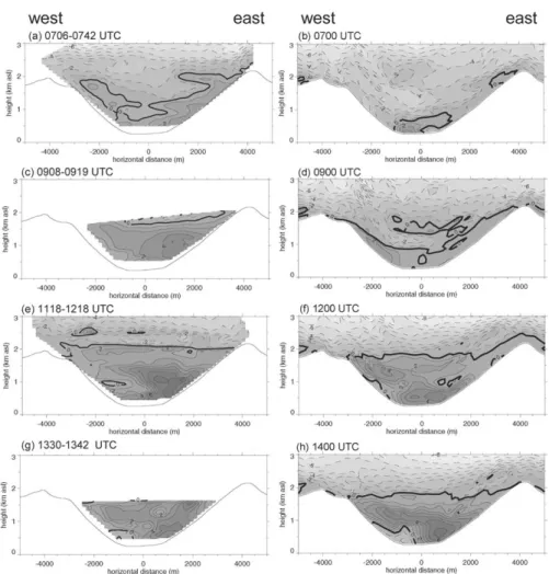
Figure 9. Interpolated cross sections of the along-valley wind component (m s−1; upvalley is positive) from aircraft data between 0706 and 0742 (a), 0908 and 0919 (c), 1118 and 1218 (e), 1330 and 1342 (g) and from model output at 0700 (b), 0900 (d), 1200 (f) and 1400 UTC (h). The bold solid line depicts the 0 m s−1 contour, solid and dashed lines refer to positive and negative contours, respectively. The contour interval is 1 m s−1. The location of the west-east cross section is depicted in Figure 1a. The horizontal distance is relative to Claro (see Figure 1).
Unfortunately, the density of the surface measurements is not sufficient to verify some aspects of the modeled surface flow patterns. Comparison between the differ-ent observed wind speeds is also complicated by the differdiffer-ent measuremdiffer-ent heights. In general, however, the valley and slope flows that are seen in the observations are captured by the simulations. Aircraft data shown later (e.g., in Figures 9e, g) also indicate disorganized flows at upper levels, and also show an isolated patch of weak downvalley directed flows during daytime on the western side of the valley, although not to such an extent as in the model.
Figure 10. Interpolated cross sections of the along-valley wind component (m s−1; upvalley is positive) from aircraft data between 1222 and 1330 UTC on the western (a) and eastern (b) sides of the valley and from model output at 1300 UTC (c). The approximate height of the ridge is indicated with a grey rectangle. Contours as in Figure 9. The location of the cross section in (a) and (b) is depicted in Figure 11. The horizontal distance is relative to Claro (see Figure 1).
Figure 11. Topography of the Riviera Valley as in Figure 1a. The aircraft flew part of the time between 1222 and 1330 UTC on the western side and part of the time on the eastern side of the valley. All the measurements taken in the western rectangle are shown in Figure 10a and all the measurements taken in the eastern rectangle are shown in Figure 10b.
We think that the complex and disorganized wind structure which includes me-andering flow regimes near the surface, is due to the topographic setting of the Riviera Valley, which does not open into a plain. This topographic setting (see Fig-ure 1) makes the flow more complicated than for a simple linear valley. The Riviera Valley flow is not entirely induced by the valley itself but is part of a larger-scale upvalley flow that splits off near the entrance of the valley and flows partly towards the Calanca and Mesolcina valleys to the north (see Figure 1). Finally, tributary valleys may also have contributed to the complex flow pattern in the Riviera Valley. 3.4.2. Spatial structure of along-valley wind
Figure 9 shows aircraft observations (left column) and simulations (right column) of the along-valley wind component in a valley cross section at four selected time intervals. Observations in the early morning show that upvalley winds occur first at the surface, and are strongest at the eastern sidewall (Figure 9a). During the day, the upvalley flow layer grows to a height of about 2 km in the early afternoon, while the wind speed maximum on the eastern side becomes more pronounced (Figures 9c, e, g). Clearly, the upvalley flow structure is horizontally inhomogeneous, with gen-erally stronger winds in the eastern part of the valley than in the western part. In the vertical direction, there are regions in the valley where a double maximum in the along-valley wind component can be seen, a maximum near the surface and one around 1 km asl. Maximum wind speeds increase during the day attaining about 7 m s−1 in the afternoon. On the western side of the valley, there is a small region with weak downvalley directed flows in the observations. These flows may be a recirculation pattern as was implied from the surface wind field in Figure 8. The layer with upvalley flow corresponds in depth to the layer that was heated in the valley atmosphere. It should be noted that the interpolated cross sections from observations were created from 1 Hz aircraft data. Before contouring, the irregular data were interpolated to a regular grid using triangulation with linear interpolation. More information on the visualization method can be found in De Wekker [13].
The onset of upvalley flows at higher elevations occurs one to two hours later in the model than in the observations (Figures 9b, d). A delay in the onset of upvalley flows in the model was also present at site A1 (Section 3.1). The modeled cross sections fail to show a wind maximum on the eastern side of the valley in the morning hours. In the afternoon, however, the modeled wind maximum moved towards the eastern side of the valley and a good agreement is found with the observed wind maxima (cf. Figures 9e and 9h). The modeled wind maximum is located closer to the surface, though. Also, modeled upvalley flows on the eastern side of the valley are about 2 m s−1 larger than observed.
Figures 10a and 10b show observed upvalley wind components on cross sec-tions in the along valley direction for the eastern and western parts of the valley between 1220 and 1330 UTC. The along-valley flight pattern of the aircraft (Fig-ure 2) shows that data are for the most part obtained over the sidewalls and may not be representative of the valley center. The data in Figures 10a and 10b are
This implies that the inhomogeneous wind structure seen in Figure 9 is not limited to this particular cross section but is also found at other locations along the valley. At some regions on the western side above about 800 m agl, flows are even directed downvalley as was also seen in the valley cross sections before.
Reiter et al. [26] observed a similar inhomogeneous behaviour of the wind structure in north-south oriented German and Austrian valleys with higher wind speeds on one side of the valley than on the other side. This behaviour was ex-plained as a result of differential heating between the two sidewalls. It is question-able whether such an explanation applies to this case since the larger wind speeds were observed to be consistently present on the eastern side of the valley during the day and did not shift from one side of the valley to the other as in Reiter et al.’s [26] observations. The shift of the modeled wind speed maximum, however, is consist-ent with Reiter’s observations and can be explained by cross-valley differences in the radiation budgets during the day.
Despite differences in the details, it is clear that the observed inhomogeneity in the wind field in the along- and cross-valley directions is well captured by the model. It can be argued that these inhomogeneities induce divergence/convergence patterns and thus vertical motion fields that enhance mixing inside the valley at-mosphere. Furthermore, the wind field differences across the valley due to the complicated topography at its southern end, may induce recirculation patterns on the scale of the valley-width, resulting in stagnant flows at locations on the valley floor or even downvalley directed flows. Such horizontal eddies (but on a larger horizontal scale) are known to exist in mountainous terrain [26].
3.5. SPATIAL POTENTIAL TEMPERATURE STRUCTURE AND CBL HEIGHTS
3.5.1. Potential temperature
Figure 12 shows aircraft observations (left column) and simulations (right column) of potential temperature in a valley cross section at four selected time intervals. The dotted lines indicate diagnosed CBL heights and will be discussed later. The observations show a cross-valley temperature structure that is rather homogeneous. The relatively stable layer below ridge height is clearly visible and is persistent
during the day as was also seen in the vertical temperature profiles at site A1. In the observations, the region near the slopes is not entirely captured by the aircraft observations since the aircraft flew no closer than about 100 m from the slopes. In the afternoon cross sections, downcurving isentropes can be seen near the slopes, especially on the eastern slope which was lit by the sun at that time. Downcurving isentropes indicate warmer temperatures near the slope which are the driving mechanism for upslope flows as illustrated e.g., in Atkinson [27]. Slope flows were observed at the surface stations on the valley sidewalls with speeds around 2 m s−1 as was shown in Section 3.3.1.
It is interesting to note that several studies have found a rather inhomogeneous temperature structure across a valley from which the existence of cross-valley cir-culations could be explained [28, 29]. Given the steepness of the Riviera Valley, it may be surprising that horizontal temperature gradients and cross-valley circula-tions were not clearly seen in the observacircula-tions. On the other hand, since 25 August was a hot day in the field campaign, turbulent mixing is expected to be strong, which could lead to a more homogeneous temperature field.
The horizontal temperature structure shows more irregularities in the model than in the observations. This is partly due to the fact that the modeled fields extend all the way to the slope. The irregularities in the modeled temperature field are also partly caused by numerical noise. This is particularly visible in the western part of the valley above ridge height in the morning. The numerical noise is caused by the treatment of horizontal diffusion in the model. Zängl [30] recently pointed out these numerical artifacts in steep terrain and presented a method to reduce the numerical errors. Besides these irregularities, the horizontally homogeneous tem-perature structure and the stable layer below ridge height are fairly well modeled. The modeled isentropes are downcurved near the slopes which is indicative of the presence of an upslope flow [27]. This deformation of the isentropes is not as clearly present in the observations.
The stability in the layer below about 1500 m is less in the model than in the ob-servations, especially in the morning hours. The model was not very successful in simulating a stable ground-based inversion in the early morning hours as discussed before.
The along-valley temperature structure between 1220 and 1330 UTC (Fi-gures 13a, b) has more irregularities in the isentropes than the cross-valley structure (Figure 12e). The inhomogeneity is even more pronounced in the modeled cross section along the valley center (Figure 13c). The differences between the eastern and western side are not very large, indicating a rather homogeneous behaviour of the temperature field in the cross-valley direction. Modeled fields show more spatial irregularities than the observations and it is difficult to assess whether these structures are real, or are artifacts of the model. As explained before, some of the irregularities may be caused by the treatment of numerical diffusion in the numerical model.
Figure 12. As in Figure 9 but for potential temperature (Kelvin). Contour interval is 1K. The dotted line indicates the CBL height determined from the Ri-method.
3.5.2. CBL heights
The dotted line in Figures 12 and 13 depicts the CBL height, determined with a Ri-method following Vogelezang and Holtslag [31]. This method calculates a modified Ri-number in a layer between the surface and incremental height levels above the surface. The CBL height is the height at which the Ri-number first ex-ceeds the value 0.25. This method has been recommended as a preferred method for the determination of CBL heights [32]. To determine CBL heights from aircraft data with the Ri-method, surface observations of potential temperature, turbulent sensible heat flux, and friction velocity are also needed. These surface observations were taken from the tower at site A1. It can be seen that the CBL height does not show significant variability over the valley floor, either in the cross-valley or in the along-valley directions. In the course of the day, the CBL height increases from
Figure 13. As in Figure 10 but for potential temperature (Kelvin). Contour interval is 1K. The dotted line indicates the CBL height determined by the Ri-method.
Figure 14. Observed versus modeled half-hourly-averaged kinematic surface sensible heat flux for all the surface stations listed in Table II.1 on 25 August 1999 between 0800 and 1600 UTC.
Figure 15. Observed (squares) and modeled (dashed line) kinematic surface sensible heat flux at site A1 (a), site B (b), and site F2 (c) on 25 August 1999. Site locations are shown in Figure 2. The shaded area indicates the range of modeled sensible heat fluxes at the nine model grid points surrounding the observation sites.
about 700 to 1300 m asl. This is higher than the CBL heights determined from visible inspection of radiosonde profiles that were shown in Figure 6. It should be mentioned though that the determination of CBL height is rather sensitive to the surface variables that are needed as input, in particular the surface potential temperature. Especially in cases where no pronounced inversion is present to cap the CBL, as in this case, there may be differences of a few hundred meters.
Prob-lems related to the determination of CBL heights in mountainous terrain with its multi-layered structure is further discussed by De Wekker [13].
Simulated CBL heights are somewhat more variable than observed heights. This is particularly so in the along-valley direction where the model simulates a complex flow pattern, including a deceleration near the middle of the valley and patches of irregular flow (as was shown in Section 3.3). This produces a region with convergence and resulting vertical motions which have an impact on the tem-perature structure and therefore the CBL height. CBL depths generally become smaller higher up on the slopes. This has been observed in other studies (e.g., [33, 34]), although still other studies (e.g., [35]) have shown an increase of CBL depth up the slope.
As the availability of surface data is limited and values vary considerably along the sloping sidewalls, CBL heights were not determined from aircraft data there. It can be expected though that CBLs are deeper over the sunlit slopes than over the shaded slopes, as predicted by the model. CBL heights cannot, by definition, be determined from the Ri-method if the surface sensible heat flux becomes negative. This explains why on the eastern sidewall in the early morning (Figure 12b), and on the western sidewall in the afternoon (Figure 12h), CBL heights are not shown.
3.6. TURBULENT SENSIBLE HEAT FLUX
Sensible heat flux was measured at all the sites listed in Table I. At a few sites latent heat flux was also measured. Inspection of the energy balance at site A1 showed that a large part of the available energy on the valley floor was used for evapo(transpi)ration, with Bowen ratios (the ratio of sensible heat flux to latent heat flux) generally smaller than 0.5. A direct comparison between modeled and observed sensible heat fluxes for all 10 surface sites is shown in Figure 14. The modeled values are taken at the grid point closest to the observation site. It is ob-vious that there is a large scatter but also that there is no clear systematic under- or overestimation. To investigate reasons for the large scatter in more detail, consider the observed and simulated turbulent sensible heat fluxes at three locations on the valley floor and west-facing slope shown in Figure 15. Observations of sensible heat flux are shown with the squares, while modeled sensible heat fluxes are shown by the dashed lines. The shaded area indicates the range of modeled sensible heat fluxes at nine grid points surrounding the observation site. It is clear that the range is large, which indicates that spatial variability of the modeled sensible heat flux is large. The variability in topographic parameters such as slope steepness and azimuth angle (or similarly, slope orientation) can explain this. This variability results in a very different timing and amount of radiation received at two points that are located close to each other (also see [36]). In the case of site F2, a site that is located near ridge level, the large variability is also due to the fact that one or more gridpoints are located on the other side of the ridge and are therefore representative for an east-facing rather than a west-facing slope. These factors, of
by the model and that there is no clear under- or overestimation of the sensible heat flux.
The spatial variability of the modeled surface sensible heat flux in the Riviera Valley (not shown) is large and follows the spatial variability of the incoming solar radiation. Sunlit slopes show larger sensible heat fluxes than shaded slopes so that there is a shift from relatively high values on the western sidewall in the morning to relatively high values on the eastern sidewall in the afternoon. There is also an increase of sensible heat flux with surface elevation, with the lowest values on the valley floor where the net radiation is also small. Figure 15 shows that there is a general tendency for sensible heat fluxes to increase with surface elevation in the observations as well. Maximum observed and simulated sensible heat fluxes are of the order of 0.1, 0.2, and 0.3 K m s−1 for site A1 (250 m asl), B (760 m asl), and F2 (2110 m asl), respectively.
4. Summary
Wind- and temperature structure, CBL height, and surface sensible heat fluxes in a steep, narrow valley were investigated with the MAP-Riviera data set and the mesocale numerical model RAMS during one fair weather day.
The vertical temperature structure is characterized by three layers. The first layer, a well-mixed layer, stays relatively shallow during the day, well below ridge height. The second layer is slightly stable. Daytime heating occurs in both the first and second layers and is more intense in the morning than in the afternoon. The third layer represents a transition zone between the valley atmosphere and the free atmosphere.
Potential temperature structure was rather homogeneous in the cross-valley dir-ection while wind structure showed a complex behaviour. A wind maximum was present on the eastern side of the valley during the entire day. This was also evident from cross sections taken in the along-valley direction. The wind and temperature structure in the along-valley direction showed a disorganized behaviour. Conditions in the Riviera Valley were not conducive to an homogeneous upvalley flow.
Aircraft, radiosonde, surface weather, and surface turbulent flux data allowed a thorough evaluation of RAMS in very steep and complex terrain using a horizontal grid spacing of 333 m. In contrast with previous studies, RAMS was initialized with a spatially heterogeneous soil moisture field, which was obtained from a hydrological model.
Simulations agree well with observed temperatures and winds at the surface. However, upvalley flows start 2 h later in the simulations than in the observations. Errors in modeled net radiation around sunrise and sunset were caused by the failure of the model to account for the effect of shadows cast by the surrounding topography.
The three-layer structure in the vertical profile of potential temperature was well simulated although the model failed to reproduce an increased stability at the top of the second layer. The temperature structure evolved differently from predicted by Whiteman’s [2] conceptual model. This may be due to the inhomogeneous wind field and associated vertical motions, which are not accounted for in the conceptual model.
Spatial temperature structure was more heterogeneous in the model than in the observations but the spatially inhomogeneous wind field was well reproduced by the model. The stronger upvalley flows on the eastern slope than on the western slope are reproduced in the modeled wind field as well. However, in the model, the wind maximum shifts from the western to the eastern side of the valley during daytime, consistent with the shift in the incoming radiation on the corresponding sidewalls, while the wind maximum remains on the eastern side of the valley in the observations. The irregular, complex flow behaviour in the Riviera Valley im-plies that one has to be careful in assuming ‘simple’ homogeneous upvalley flow conditions in these types of terrain, as is often done, for example, in mass budget studies.
CBL heights diagnosed with the Ri-method from simulations and observations correspond well over the valley floor, but can differ significantly from CBL heights diagnosed from vertical temperature profiles only. The maximum depth of the CBL is around 1000 m and the CBL top does not show large spatial variability along and across the valley floor.
The comparison of modeled and observed surface turbulent sensible heat fluxes exhibits large scatter. Differences in slope steepness and orientation between meas-urement sites and the locations of model grid points can explain this scatter, while the inherent uncertainty of taking turbulence measurements in complex terrain makes it difficult to compare simulated and observed values. Given these prob-lems, it is encouraging that observed sensible heat fluxes lie within the range of modeled sensible heat fluxes that result from taking values from the nine grid points surrounding the measurement sites.
Overall, the MAP-Riviera field study provided a data set that is particularly well-suited for the evaluation of a mesoscale model in complex terrain. Given the assumption of flat and homogeneous terrain in the parameterization schemes of
of DS and SdW in the MAP-Riviera field study.
We would like to thank M. Andretta, A. Weigel, A. Weiss, and M. Zappa for providing MAP data, and K. Jasper for providing soil moisture output from the hydrological model WaSiM-ETH. Dr André Prevôt is acknowledged for allowing SdW to finalize this paper during a post-doctoral appointment at the Paul Scher-rer Institute. We would like to thank Dr C. David Whiteman for providing useful comments on the manuscript.
Support in the revision stage of this paper was received from the Department of Energy (DOE) under the auspices of the Atmospheric Sciences Program of the Environmental Sciences Division of the Office of Biological and Environmental Research under Contract DE-AC06-76RLO 1830 at the Pacific Northwest National Laboratory (PNNL). PNNL is operated for the US DOE by Battelle Memorial Institute.
References
1. Whiteman, C.D.: 1990, Observations of thermally developed wind systems in mountainous terrain. W. Blumen (ed.), Atmospheric Processes over Complex Terrain, Meteorol. Monogr., 23 (no. 45), Amer. Meteor. Soc., Boston, Massachusetts, Chapter 2, pp. 5–42.
2. Whiteman, C.D.: 1982, Breakup of temperature inversions in deep mountain valleys: Part 1. Observations, J. Appl. Meteorol.., 21, 270–289.
3. Freytag, C.: 1987, Results from the MERKUR experiment: Mass budget and vertical motions in a large valley during mountain and valley wind, Meteorol. Atmos. Phys. 37, 129–140. 4. Rotach, M.W., Calanca, P., Graziani, G., Gurtz, J., Steyn, D.G., Vogt, R., Andretta, M.,
Christen, A., Cieslik, S., Connolly, R., De Wekker, S.F.J., Galmarini, S., Kadygrov, E.N., Kadygrov, V., Miller, E., Neininger, B., Rucker, M., van Gorsel, E., Weber, H., Weiss A. and Zappa, M.: 2004, turbulence structure and exchange processes in an Alpine valley: The Riviera project, Bull. Amer. Meteorol. Soc. 85, 1367-1385.
5. Bougeault, P., Binder, P., Buzzi, A., Dirks, R., Houze, R., Kuettner, J., Smith, R.B., Steinacker, R. and Volkert, H.: 2001, The MAP special observing period, Bull. Amer. Meteorol. Soc. 82, 433–462.
6. Neininger, B., Fuchs, W., Bäumle, M., Volz-Thomas, A., Prévôt, A.S.H. and Dommen, J.: 2001, A small aircraft for more than just ozone: MetAir’s ’Dimona’ after ten years of evolving development. In: Proceedings of the 11th Symposium on Meteorological Observations and Instrumentation, Albuquerque, NM, 14–19 January 2001, pp. 123–128.
7. Furger, M., Dommen, J., Graber, W.K., Poggio, L., Prévôt, A., Emeis, S., Grell, G., Trickl, T., Gomiscek, B., Neininger, B. and Wotawa, G.: 2000, The VOTALP Mesolcina Valley Campaign 1996 – concept, background, and some highlights. Atmos. Environ. 34, 1395–1412.
8. Pielke, R.A., Cotton. W.R., Walko, R.L., Tremback. C.J., Lyons, W.A., Grasso, L.D., Nich-olls, M.E., Moran, M.D., Wesley, D.A., Lee, T.J. and Copeland, J.H.: 1992, A comprehensive meteorological modeling system – RAMS. Meteorol. Atmos. Phys. 49, 69–91.
9. Cotton, W.R., Pielke Sr., R.A., Walko, R.L., Liston, G.E.:, Tremback, C.J., Jiang, H., McAnelly, R.L., Harrington, J.Y., Nicholls, M.E., Carrio, G.G. and McFadden, J.P.: 2003: RAMS 2001: Current status and future directions, Meteorol. Atmos. Phys. 82, 5–29.
10. Walko, R.L., Band, L.E., Baron, J., Kittel, T.G.F., Lammers, R., Lee, T.J., Ojima, D., Pielke Sr., R.A., Taylor, C., Tague, C., Tremback, C.J. and Vidale, P.L.: 2000, Coupled atmosphere– biophysics–hydrology models for environmental modeling, J. Appl. Meteorol. 39, 931–944. 11. Davies, H.C.: 1976, A lateral boundary formulation for multi-level prediction models, Quart.
J. Roy. Meteorol. Soc. 102, 405–418.
12. BFS (Bundesamt für Statistik): 1993, Die Bodennutzung der Schweiz. Arealstatistik 1979/85, Bern.
13. De Wekker, S.F.J.: 2002, Structure and Morphology of the Convective Boundary Layer in Mountainous Terrain, Ph.D. Dissertation, The University of British Columbia, BC, Canada, 191 pp.
14. Grasso, L.D.: 2000, A numerical simulation of dryline sensitivity to soil moisture, Mon. Wea. Rev. 128, 2816–2834.
15. Jacobson, M.Z.: 1998, Effects of soil moisture on temperatures, winds, and pollutant concen-trations in Los Angeles, J. Appl. Meteorol. 38, 607–616.
16. Jasper, K.: 2002, Hydrological Modelling of Alpine River Catchments Using Output Variables from Atmospheric Models, Diss. ETH No. 14385, Zurich.
17. Zappa, M, Matzinger, N. and Gurtz, J.: 2000, Hydrological and meteorological measurements at Claro (CH) – Lago Maggiore target area in the MAP-SOP 1999 RIVIERA experiment includ-ing first evaluation. In: B. Bacchi and R. Ranzi (eds.) Hydrological Aspects in the Mesoscale Alpine Programme-SOP Experiment, Technical Report of the Dept. of Civil Engineering – Univ. of Brescia, 10(2).
18. Frei, C. and Schär, C.: 1998, A precipitation climatology of the Alps from high-resolution rain-gauge observations, Int. J. Climatol. 18, 873–900.
19. Andretta, M., Weiss, A., Kljun, N. and Rotach, M.W.: 2001, Near-surface turbulent momentum flux in an Alpine valley: Observational results, MAP Newslett. 15, 122–125.
20. Barry, R.G.: 1992, Mountain Weather and Climate, 2nd edition, Routledge, 402 pp. 21. Whiteman, C.D.: 2000, Mountain Meteorology, Oxford University Press, 355 pp.
22. Stull, R.B.: 1988, An Introduction to Boundary Layer Meteorology, Kluwer Academic Publish-ers, Dordrecht, pp. 666.
23. Kondratyev, J.: 1969, Radiation in the Atmosphere, Academic Press, New York, 912 pp. 24. Colette, A.G., Katopodes Chow, F. and Street, R.L.: 2003, A numerical study of
inversion-layer breakup and the effects of topographic shading in idealized valleys, J. Appl. Meteorol. 42, 1255–1272.
25. Weigel, A.H. and Rotach, M.W.: 2003, On the turbulence structure in a daytime alpine valley atmosphere. In: Preprints ICAM/MAP 2003, 19–23 May 2003, Brig, Switzerland, pp. 162–165. 26. Reiter, R., Müller, H., Sladkovic, R. and Munzert, K.: 1983, Aerologische Untersuchungen der tagesperiodischen Gebirgswinde unter besonderer Berücksichtigung des Windfeldes im Talquerschnitt. Meteorol. Rundsch. 36, 225–242.
27. Atkinson, B.W.: 1981: Mesoscale Atmospheric Circulations, Academic Press, London, 279 pp. 28. Hewson, E.W. and Gill, G.C.: 1944, Meteorological Investigations in Columbia River Valley
Atmos. Environ. 32, 1323–1348.
34. De Wekker, S.F.J.: 1995, The Behaviour of the Convective Boundary Layer Height over Orographically Complex Terrain. Unpublished MS Thesis University of Karlsruhe, Ger-many/Wageningen Agricultural University, the Netherlands, 74 pp.
35. Moll, E., 1935, Aerologische Untersuchungen periodischer Gebirgswinde in V-förmigen Alpentälern, Beitr. Physik f. Atmos. 22, 177–197.
36. Matzinger, N., Andretta, M., van Gorsel, E., Vogt, R., Ohmura, A. and Rotach, M.W: 2003, Surface radiation budget in an Alpine valley, Quart. J. Roy. Meteorol. Soc. 129, 877–895. 37. Turnipseed, A.A., Blanken, P.D., Anderson, D.E. and Monson, R.K.: 2002, Energy budget
above a high-elevation subalpine forest in complex topography, Agric. For. Meteorol. 110, 177–201.