Impact of the chemical description on Direct Numerical Simulation and Large Eddy Simulation of turbulent combustion in industrial aero-engines

HAL Id: tel-00662813

https://tel.archives-ouvertes.fr/tel-00662813

HAL is a multi-disciplinary open access

archive for the deposit and dissemination of sci-entific research documents, whether they are pub-lished or not. The documents may come from

L’archive ouverte pluridisciplinaire HAL, est destinée au dépôt et à la diffusion de documents scientifiques de niveau recherche, publiés ou non, émanant des établissements d’enseignement et de

Simulation and Large Eddy Simulation of turbulent

combustion in industrial aero-engines

Benedetta Giulia Franzelli

To cite this version:

Benedetta Giulia Franzelli. Impact of the chemical description on Direct Numerical Simulation and Large Eddy Simulation of turbulent combustion in industrial aero-engines. Fluid mechanics [physics.class-ph]. Institut National Polytechnique de Toulouse - INPT, 2011. English. �tel-00662813�

Réf. CERFACS : N° d’ordre :

T

T

T

H

H

H

E

E

E

S

S

S

E

E

E

D

D

D

O

O

O

C

C

C

T

T

T

O

O

O

R

R

R

A

A

A

T

T

T

D

D

D

E

E

E

L

L

L

’

’

’

U

U

U

N

N

N

I

I

I

V

V

V

E

E

E

R

R

R

S

S

S

I

I

I

T

T

T

É

É

É

D

D

D

E

E

E

T

T

T

O

O

O

U

U

U

L

L

L

O

O

O

U

U

U

S

S

S

E

E

E

Délivré par Institut National Polytechnique de Toulouse Discipline ou spécialité : Energie et Transferts

O. GICQUEL H. PITSCH W. JONES J-F. PAUWELS E.S. RICHARDSON A. ROUX B. CUENOT JURY

Professeur - Ecole Centrale de Paris Professeur - RWTH Aachen University Professeur - Imperial College of London Professeur - Université Lille 1

Chercheur - University of Southampton Ingénieur - Turbomeca

Chercheur Senior au CERFACS

Rapporteur Rapporteur Examinateur Examinateur Examinateur Invité Directeur de thèse

École doctorale : Mécanique, Energétique, Génie civil, Procédés Unité de recherche : CERFACS

Directeur de Thèse : Bénédicte CUENOT Co-encadrant : _{Eleonore RIBER}

Par Benedetta Giulia FRANZELLI Date de soutenance : 19 septembre 2011

IMPACT OF THE CHEMICAL DESCRIPTION ON DIRECT NUMERICAL

SIMULATIONS AND LARGE EDDY SIMULATIONS OF TURBULENT

Résumé

Le développement de nouvelles technologies pour le transport aérien moins polluant est de plus en plus basé sur la simulation numérique, qui nécessite alors une description fiable de la chimie.

Pour la plupart des carburants, la description de la combustion nécessite des mécanismes détaillés mais leur utilisation dans une simulation numérique de combustion turbulente est limitée par le coût calcul. Des mécanismes cinétiques réduits et des méthodes de tabulation ont été proposés pour surmonter ce problème. Ces descriptions chimiques simplifiées ayant été développées dans le cadre de configurations laminaires, cette thèse propose de les évaluer dans des configurations turbulentes: une DNS de flamme prémélangée méthane/air de type Bunsen et une LES d’un brûleur expérimental. Les mécanismes sont analysés en termes de structure de flamme, paramètres de flamme globaux, longuer de flamme, prediction des concentrations en espèces majoritaires et des émissions polluantes.

Une méthodologie pour évaluer a priori la capacité d’un mécanisme à prédire correctement des phénomènes chimiques tridimensionnels est proposée en se basant sur les résultats de flammes laminaires monodimensionnelles non étirées et étirées. Il ressort que, d’une part, pour constru-ire un mécanisme réduit, il est nécessaconstru-ire de faconstru-ire un compromis entre coût calcul, robustesse et qualité des résultats. D’autre part, la qualité des résultats de DNS et LES de configurations tridimensionnelles turbulentes peut être anticipée par une analyse du comportement des sché-mas réduits dans des configurations simplifiées de flammes monodimensionnelles laminaires non étirées et étirées.

Mots-clés : mécanisme cinétique réduit, combustion turbulente, simulation numérique directe, simulation aux grandes échelles.

Abstract

A growing need for numerical simulations based on reliable chemistries has been observed in the last years in order to develop new technologies which could guarantee the reduction of the enviromental impact on air transport.

The description of combustion requires the use of detailed kinetic mechanisms for most hydro-carbons. Their use in turbulent combustion simulation is still prohibitive because of their high computational cost. Reduced chemistries and tabulation methods have been proposed to over-come this problem. Since all these reductions have been developed for laminar configurations, this thesis proposes to evaluate their performances in simulations of turbulent configurations such as a DNS of a premixed Bunsen methane/air flame and a LES of an experimental PREC-CINSTA burner. The mechanisms are analysed in terms of flame structure, global burning parameters, flame length, prediction of major species concentrations and pollutant emissions. An a priori methodology based on one-dimensional unstrained and strained laminar flames to evaluate the mechanism capability to predict three-dimensional turbulent flame features is therefore proposed. On the one hand when building a new reduced scheme, its requirements should be fixed compromising the computational cost, the robustness of the chemical descrip-tion and the desired quality of results. On the other hand, the quality of DNS or LES results in three-dimensional configurations could be anticipated testing the reduced mechanism on laminar one-dimensional premixed unstrained and strained flames.

!

!

!

!

"!#$%&'%()!#*&')$+,,%!

!

!

!

!

!"#$%&$'())$%*+$,%&($--$%./#",0$%

-)('+!",%./%+$%!

Contents

Introduction

1

I

General features on turbulent combustion

13

1 Turbulent premixed combustion 15

1.1 Conservation equations for reacting flows . . . 18

1.1.1 Filtering and Large Eddy Simulation . . . 21

1.2 Turbulent premixed combustion . . . 22

1.2.1 Combustion regimes . . . 24

1.2.2 Turbulent flame speed . . . 28

1.2.3 Combustion modelling for LES . . . 29

1.3 Chemistry for turbulent combustion . . . 32

1.3.1 Skeletal mechanisms . . . 33

1.3.2 Reduced chemical mechanisms . . . 33

1.3.3 Manifold generation methods . . . 35

1.4 CFD tools . . . 36

II

Chemistry models for turbulent combustion

39

2.2 Unstrained premixed flames . . . 45

2.3 Strained premixed flames . . . 55

3 Chemistry for premixed methane/air flames 61 3.1 Reduced mechanisms for laminar premixed flame . . . 61

3.1.1 Simplified transport properties . . . 62

3.1.2 The two-step mechanisms: 2S_CH4_BFER and 2S_CH4_BFER* . 64 3.1.3 The four-step mechanisms: JONES and JONES* . . . 70

3.1.4 The analytical mechanisms: PETERS and PETERS* . . . 73

3.1.5 The SESHADRI and SESHADRI* mechanisms . . . 75

3.1.6 The LU mechanism . . . 77

3.1.7 Implementation of reduced mechanisms in CFD tools . . . 77

3.2 Comparison between reduced mechanisms . . . 81

3.2.1 Comparison between reduced mechanisms on unstrained flames 81 3.2.2 Comparison between reduced mechanisms on strained flames . . 88

3.3 The FPI_TTC tabulation method . . . 95

3.4 Towards turbulent combustion: generalization of the thickened flame method . . . 98

3.5 Conclusions . . . 101

III

Validation and impact of chemistry modeling in unsteady

turbulent combustion simulations

105

4.1.1 Numerical configuration . . . 108

CONTENTS

4.1.3 Comparison of the different reduced mechanisms . . . 112

4.2 DNS of homogeneous isotropic turbulent field with flame . . . 120

4.2.1 Numerical configuration and initialization of the HIT field . . . . 121

4.2.2 Temporal evolution . . . 123

4.2.3 Comparison of the different reduced mechanisms . . . 126

4.2.4 Preliminary conclusions on academic configurations . . . 134

4.3 DNS of stationary lean premixed Bunsen flame . . . 136

4.3.1 Numerical configuration . . . 137

4.3.2 Results . . . 138

4.4 Conclusions . . . 145

5 Impact of the reduced chemical mechanisms on LES of a lean partially pre-mixed swirled flame 149 5.1 The PRECCINSTA burner . . . 150

5.1.1 Experimental measurements . . . 152

5.2 The numerical setup . . . 153

5.2.1 Mesh, numerical method and boundary conditions . . . 153

5.2.2 Artificially thickened flame model . . . 156

5.3 Analysis of results . . . 156

5.3.1 Mixing . . . 158

5.3.2 Mean and fluctuating quantities . . . 162

5.3.3 Mean flame surface . . . 170

5.3.4 Towards pollutant emission prediction: the post-flame zone . . . 172

5.3.5 Impact of mesh refinement . . . 176

5.4 General remarks and conclusions . . . 180 6 Large-Eddy Simulation of instabilities in a lean partially premixed swirled

6.1 Article . . . 184

6.1.1 The swirled premixed burner configuration . . . 185

6.1.2 Large Eddy simulation for gas turbines . . . 187

6.1.3 Results and discussions . . . 194

6.1.4 Conclusions . . . 201

General conclusions

201

Bibliography

215

Acknowledgements

228

Partie en français

231

Appendix A

245

Nomenclature

Abreviations

ACARE Advisory Council for Aeronautics Research in Europe

CFD Computational Fluid Dynamics

CPU Central processing unity

DNS Direct Numerical Simulation

DTFLES Dynamically thickened flame method for LES

ECCOMET Efficient and Clean Combustion Experts Training

FPI Flame Prolongation of ILDM

HIT Homogeneous isotropic turbulence

ILDM Intrinsic Low-Dimensional Manifold

ISAT In Situ Adaptive Tabulation

LES Large Eddy Simulation

LPM Lean Pre-Mixed

PAH Polycyclic Aromatic Hydrocarbons

PCM Presumed Conditional Moments

PDF Probability density function

PEA Pre-Exponential Adjustment

PRECCINSTA PREdiction and Control of Combustion INSTAbilities

for industrial gas turbines

QSS Quasi-steady state

QUANTIFY Quantifying the Climate Impact of Global and European

Transport Systems

RANS Reynolds-Averaged Navier-Stokes

RMS Root mean square

TFLES Thickened flame method for LES

Greek letters

αP Exponent for flame speed dependency on pressure [− ]

αT Exponent for flame speed dependency on temperature [− ]

⇥j Temperature exponent for reaction j [− ]

∆H0

j Enthalpy change of reaction j [ J ]

∆h0

f,k Mass formation enthalpy of species k [ J/Kg ]

∆S0

j Entropy change of reaction j [ J/K ]

⌅ Diffusive flame thickness [ m ]

⌅L Thermal flame thickness [ m ]

⌅B

L Blint flame thickness [ m ]

⌅r Reaction zone thickness [ m ]

⌅ij Component (i, j) of the Kronecker delta [ - ]

˙

ωc Reaction rate for the progress variable c [ 1/s ]

˙

ωF Fuel consumption rate [ kg/m3/s ]

˙

ωk Mass reaction rate of species k [ kg/m3/s ]

˙

ωT Heat release due to combustion [ J/m3/s ]

˙

ω⇣

T Heat release due to combustion [ J/m3/s ]

Λ Flame front length [ m ]

NOMENCLATURE

Λ◆ Reduced flame front length [− ]

Λ₀ Flame front length at the initial time [ m ]

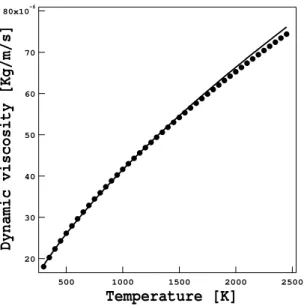
µ Mixture dynamic viscosity [ Kg/m/s ]

ν Mixture cinematic viscosity [ m2_{/s ]}

ν⇣⇣

k j Molar stoichiometric coefficient of species k for the

backward reaction j [ - ]

ν⇣

k j Molar stoichiometric coefficient of species k for the

forward reaction j [ - ]

φ Equivalence ratio [_{− ]}

Mixture density [ kg/m3_]

k Density of species k [ kg/m3]

Σ Surface density [ 1/s ]

↵K Kolmogorov time scale [ s ]

↵c Chemical time scale [ s ]

↵t Integral time scale [ s ]

↵ij Component (i,j) of the viscous force tensor [ N/m2]

Non-dimensional numbers

Da Damköhler number

Ka Karlovitz number

Kar Karlovitz number based on the reaction zone thickness

LeF Fuel Lewis number

Lek Lewis number of species k

Mc

a Markstein number for consumption speed

Md

a Markstein number for displacement speed

Pr Prandtl number

Ref Flame Reynolds number

Sck Schmidt number for species k

Roman letters

[Xk] Molar concentration of species k [ mol/m3]

˙Q Heat source term [ J/m3_{/s ]}

n Flame surface normal [− ]

E Efficiency factor [− ]

F Thickening factor [_{− ]}

Jk

i Component i of the molecular diffusive flux of species k [ Kg/m

2_{/s ]}

Mk Name of species k [ - ]

Qj Progress rate of reaction j [ mole/m3/s ]

k Turbulent kinetic energy [ m2_/s2_]

SC Flamelet consumption speed [ m/s ]

a Strain rate [ 1/s ]

AL Area of the unwrinkled flame surface [ m ]

AT Area of the wrinkled flame surface [ m ]

Af j Pre-exponential factor for forward reaction j [ cgs ]

c Progress variable [− ]

Cpk Specific heat capacity of species k at constant pressure [ J/(Kg K) ]

Dk Molecular diffusivity of species k [ m/s ]

Dth Heat diffusivity [ m/s ]

Eaj Activation energy for reaction j [ cal/mol ]

Fi Component i of the body force [ N/m2]

fk,j Component i of the volume force on species k [ N/m2]

NOMENCLATURE

hs,k Mass sensible enthalpy of species k [ J/Kg ]

I0 Burning intensity [− ]

k Stretch [ 1/s ]

k_K Kolmogorov wave number [ 1/m ]

ke Integral wave number [ 1/m ]

Keq Equilibrium reaction constant [− ]

Kf j Forward reaction constant for reaction j [ cgs ]

Krj Reverse reaction constant for reaction j [ cgs ]

l Characteristic domain length [ m ]

lK Kolmogorov length scale [ m ]

lt Integral length scale [ m ]

lt Turbulent length scale [ m ]

m Mixture mass [ kg ]

mk Mass of species k [ kg ]

n Number of moles [ mol ]

n⇣

k j Forward order for reaction j and species k [− ]

n⇣⇣

k j Backward order for reaction j and species k [− ]

nk Number of moles of species k [ mol ]

p Pressure [ N/m2_]

pk Partial pressure of species k [ N/m2]

qi Component i of energy flux [ J/m2/s ]

R Perfect gas constant [ J/mol/K ]

s Mass stoichiometric ratio [− ]

Sa Absolute speed [ m/s ]

Sd Displacement speed [ m/s ]

S◆

d Density-weighted displacement speed [ m/s ]

SL Propagation speed [ m/s ]

ST Turbulent flame speed [ m/s ]

sk Mass entropy of species k [ J/K/Kg ]

T Mixture temperature [ K ]

u⇣ _{root mean square of velocity [ m/s ]}

u_K Kolmogorov speed [ m/s ]

ui Component i of velocity vector [ m/s ]

up Turbulent speed [ m/s ]

V Mixture volume [ m3_]

Vc

i Correction velocity in direction i [ m/s ]

Vk,i Species diffusion velocity in direction i for species k [ m/s ]

W Mean molecular weight of the mixture [ kg/mol ]

Wk Atomic weight of species k [ kg/mol ]

Xk Molar fraction of species k [ - ]

Yk Mass fraction of species k [ - ]

z Mixture fraction [_{− ]}

Introduction

Challenges of combustion in aeronautical engines

Air transport moves over 2.2 billion passengers annually and generates a total of 32 million jobs corresponding to a global economic impact estimated at 3.560 billion of euros. Unfortunately, the fossil fuel combustion typically used in aeronautical engines has a negative impact on climate being characterized by emission of pollutant species:

• Oxides of carbon such as the carbon monoxide CO, which is highly toxic com-bining with hemoglobin and attacking the delivering of oxygen to bodily tissues,

and the carbon dioxide CO2which is not toxic and it is one of the greenhouse gas

responsible for climate change.

• Oxides of nitrogen such as the nitric oxide NO and the nitrogen dioxide NO2

(generally referred as NOx) and the nitrous oxide N2O. They have a strong climate

impact, i.e. formation of acid rain, and they are greenhouse gases participating in ozone layer depletion.

• Oxides of sulfur such as the sulfur dioxide SO2 and the sulfur trioxide SO3,

precursors of acid rain and atmospheric particulates.

• Highly toxic soot having a strongly negative impact on human health.

• Unburned hydrocarbon such as alkanes, ketones and alcohols due to an incom-plete oxidation of hydrocarbons caused by a low temperature value or a too large heterogeneity of the mixture.

Since 2001 the ACARE1 _{establishes the roadmap for aeronautical technology}

de-velopment in the European Union. It aspires at a better technology linked to social

1_{The Advisory Council for Aeronautics Research in Europe (ACARE) is composed by representation}

thematic (cleaner environment, safer travel and more security) as well as at the ben-efits of a more competitive Europe. In the 2008 Addendum to the Strategic Research Agenda, three important areas have been identified for increased priority:

• Environment: the transport impact is represented in Fig. 1 in terms of net

temper-ature change for four future times2_{. Even if the aviation contribution is relatively}

small compared to road transport and producing only 2% of human-induced

CO2 emissions, its emissions have to be controlled since air transport is quickly

growing by a factor of 4_{− 5% per year and emissions at altitude have an effect on}

climate change greater than the industry CO2emissions alone.

Figure 1 - Contribution from a one-year pulse of current (year 2000) emissions to net future temperature change (mK) for each transport mode for 4 future times (20, 40, 60 and 100 years) [22].

Developing a sustainable aviation system is an urgent thematic concerning global climate change, local noise and air quality. The environmental objectives fixed by the ACARE in the 2020 horizon are:

– reduction of CO2 emission by 50% per passenger kilometer (assuming

kerosene remains the main fuel in use);

– perceived noise reduction to one half of the current average levels;

– reduction of NOxemissions by 80%;

– reduction of other emissions: soot, CO, particulates, etc.

– minimization of the industry impact on the global environment.

2_{Results from the final activity report of the QUANTIFY (Quantifying the Climate Impact of Global}

INTRODUCTION

• Alternative Fuels: total energy demand is increasing significantly due to popu-lation growth and developing economies whereas the world’s reserves of oil are decreasing. The use of new alternative fuels in aviation is not yet a necessity but a study of the specifications of these potential new fuels is required in order to pre-pare and adapt the aeronautical systems to them. Moreover, their environmental impact has to be carefully analyzed.

• Security: measures to increase the security of passengers at airports are also proposed.

Reduction of pollutant emissions is one of the main objectives of the ACARE. The short-term and long-short-term climate impacts of aviation have been evaluated in the QUANTIFY

project including those of long-lived greenhouse gases like CO2 and N2O, of ozone

precursors and particles, as well as contrail and cirrus cloud impact [22]. Temperature changes due to aviation have been estimated for various years after the emissions with

standard emissions and with 20% reduced CO2and NOxemissions (see Fig. 2).

Devel-oping new technologies, CO2emissions per passenger-kilometer could be reduced and

the climate impact would decrease on the long time horizons.

a. b.

Figure 2 - Comparison of temperature change for various years after the emissions due to aviation with standard emissions for the year 2000 and with reduced CO2and NOxemissions (−20%) [22]. a)

Temperature change per compound and b) specific climate impact of passenger modes per passenger-kilometer.

The experimental and numerical study of aeronautical engines greatly contributes to the development of new technologies which could guarantee the expected 20%

phenomena taking place into the combustion chamber such as the production of pollu-tants is one fundamental step for minimizing the environmental impact and ensuring the security of the aeronautical systems using alternative fuels.

Turbulent combustion is characterized by multiple aspects: spray dynamics

and two-phase flows, radiation effect and wall heat losses, interaction of heat and sound...However, in a very simplified way, it describes the interaction between a turbulent flow and a flame: none of these improvements is useful if the two funda-mental bricks, turbulence and chemistry, are not correctly described. Modeling the chemical phenomena and their interaction with turbulence is one of the major problem of combustion.

Chemical description in turbulent combustion

Detailed kinetic mechanisms, comprising hundreds of species and thousands of re-actions, are available for most hydrocarbons [148]. They correctly predict multiple aspects of flames over a wide range of cases (i.e. one-dimensional flame structure, gas composition in a stirred reactor, ignition delay, etc...). Unfortunately, using these mechanisms in turbulent combustion simulation is still prohibitive:

• theoretical difficulties: in most combustion models, the coupling between turbu-lence and combustion is generally accounted for through the comparison of a sin-gle turbulent time to the characteristic chemical time. Since detailed mechanisms are characterized by very different time scales (i.e. fuel oxidation is governed

by fast reactions whereas NOx production is the result of slow reactions), this

coupling is not straightforward.

• computational costs: the computational time drastically increases with the num-ber of species to be solved. Moreover, complex schemes are usually very stiff and demand specific (implicit) algorithms to avoid unreasonably small time steps. Two approaches have been proposed to overcome this problem:

• Reduced chemistry: simplification of a detailed mechanism in order to obtain ac-curate chemical behavior with less species and reactions. They could be classified as:

– Global or semi-global fitted schemes [171, 63, 144]: they are generally built

to correctly reproduce global quantities for premixed flames such as flame speed and burnt gas state. On the one side, these mechanisms are generally easy to build for a wide range of initial conditions, their implementation in

INTRODUCTION

a CFD solver is usually straightforward and they are very robust. On the other side, only global quantities are correctly predicted and all information on intermediate species disappears.

– Analytical mechanisms [116, 41, 40, 103, 21]: they have been proposed to

include more details on the flame such as its structure or the ignition delay. A detailed understanding of the relevant chemistry is required to build this kind of mechanism in order to remove the chemical steps that are useless for specific conditions. These mechanisms provide a physical insight of the chemical processes and some of the intermediate species are correctly de-scribed. Unfortunately, their implementation and use in a CFD solver is not easy since they are generally characterized by algebraic relations which are difficult to treat numerically and their computational cost is higher compared to global schemes.

• Tabulated chemistry: technique based on the idea that the variables of a chemical mechanism are not independent. The flame structure is studied as function of some few variables (ex. temperature, mixture fraction) used to build a flame database [102, 69, 160, 49]. All the intermediate radicals are available during the computation but their concentrations depend on the information stored into the look-up table, i.e. on the prototype flame chosen to build the table. Handling the table is difficult when simulating complex industrial configurations:

– its dimension grows rapidly with the number of parameters that have to be

taken into account. Solution based on algorithms that dynamically build the table (In Situ Adaptive Tabulation ISAT methods) [126] or on the self-similarities of the flame structure [128, 161, 60] have been proposed;

– determining the prototype flame to create the table could be a complicated

task when the combustion regime is unknown.

A growing need for simulations based on reliable chemistries has been underlined in the last years [77] since restrictions on pollutant emissions motivate request for more accurate results. As a consequence, these simplified chemical descriptions should be carefully used when simulating three-dimensional turbulent complex flames:

• in order to reduce the computational cost, some pieces of information are ne-glected and accuracy could be affected;

• all these reductions have been developed and evaluated for laminar configura-tions and their impact on turbulent unsteady flames has not yet been completely evaluated.

A first attempt to characterize the impact of reduced mechanisms on turbulent combus-tion was proposed by Hilka et al. [78] carrying computacombus-tions of an interaccombus-tion between

a vortex pair and a lean methane/air premixed flame with a detailed mechanism (17 species and 52 reactions) and a semi-global scheme (9 species and 4 reactions). Discrep-ancies between the two mechanisms were underlined on this unsteady configuration

for the heat release and the production rates of CO, CO2and H2O species. They were

mainly due to the different responses of the mechanisms to strain rate and curvature, and a coupling between chemistry and differential diffusion effects leading to changes in the local composition, and not only to pure kinetics.

At the same time, Baum et al. [13, 14] analyzed the response of a hydrogen/oxygen premixed flame to a homogeneous isotropic turbulent field comparing a simple-step chemistry using constant Lewis numbers with a complete scheme (9 species and 19 reactions) and zeroth-order approximation of the species diffusion velocities. Dis-crepancies were detected for the flame structure linked to strain rate and curvature response.

The impact of simplified mechanisms has been analyzed on other two-dimensional and three-dimensional configurations [77, 130, 155, 20].

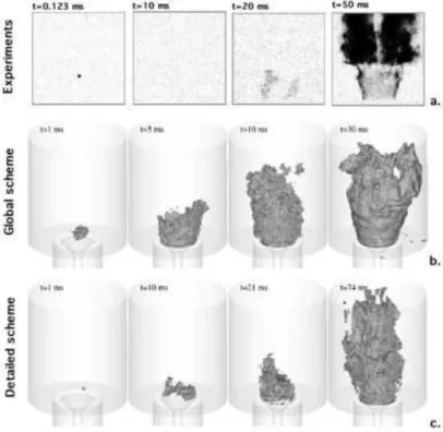
Figure 3 - Instantaneous pictures of an ignition event for a methane/air flame in a bluff-body configuration. Experimental results by [1] (a.) are compared to numerical results [155] using a global

scheme (b.) and a detailed mechanism (c.).

Simulations of forced ignition of a non-premixed bluff-body methane/air flame by Triantafyllidis et al. [155] showed that a single-step mechanism could reproduce the experimental results [1] with a reasonable accuracy but a better agreement was found

INTRODUCTION

when using a detailed scheme based on 16 species (Fig. 3). Moreover, in [20] it was found that the numerical results of a supersonic hydrogen-air autoignition stabilized flame greatly depend on the simplified mechanism used (Fig. 4).

a. b.

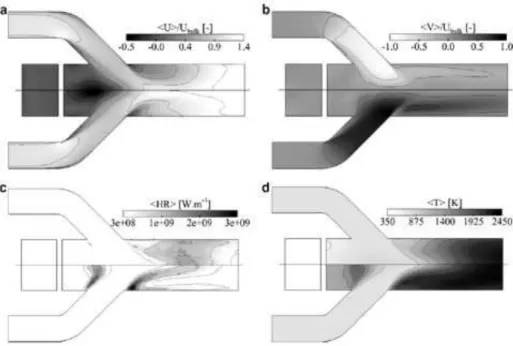
Figure 4 - Instantaneous and mean a) temperature and b) HO2mass fraction in the center plane of the flame for three different chemistries [20].

Simulations of a side-dump ramjet combustor using a classical one-step scheme and a similar scheme which corrected the flame speed for rich laminar premixed mixture suggested that the chemical scheme not only affects the mean flow field (see Fig. 5) but also the description of thermo-acoustic instabilities [130]. However, no indication was given about the required characteristics of a reduced mechanism to correctly reproduce the main features of the combustion phenomenon.

Finally, Cao and Pope[34] have studied the performance of seven different chemical mechanisms in joint PDF model calculations of the Barlow and Frank [12] non-premixed piloted jet flames D, E and F. A good agreement with experimental results is achieved when using the most complex schemes (called GRI3.0, GRI2.11 and skeletal) whereas the simplest mechanisms (named S5G211, Smooke, ARM1 and ARM2) display signif-icant inaccuracies in term of temperature and species concentrations, causing in some cases an unphysical extinction of the flame (Fig. 6).

Figure 5 - Mean flow quantities of the side-dump ramjet combustor calculated by Roux et al. [130]. For each subfigure, top: corrected one-step scheme and bottom: standard one-step scheme. a) Axial velocity,

b) radial velocity, c) rate of heat release and d) temperature.

Figure 6 - Burning indices of temperature versus jet velocity for the Barlow and Frank flames D,E and F [12] calculated by Cao and Pope [34]. Comparison between experimental data and seven chemical

mechanisms.

Even if the importance of a good chemical description has already been underlined in complex configurations, the characteristics of the chemistry model required to cor-rectly reproduce turbulent flames in unsteady calculations have not been completely identified.

INTRODUCTION

Contribution of this thesis

In this thesis, the impact of the chemistry description using reduced kinetic mecha-nisms is analyzed on turbulent premixed flames in the context of unsteady simulation approaches. Using reduced kinetic mechanisms leads to possible errors on quantities of interest such as major species concentration and temperature, flame structure and its position, its response to turbulence as well as the description of pollutant emissions. Identifying and quantifying these errors are of primary importance for the development of simulation tools.

More precisely, this thesis has two main objectives:

• The development of a methodology to build semi-global schemes that correctly predict the flame speed and the burnt gas state for premixed one-dimensional laminar flames on a wide range of pressure, initial temperature and equivalence ratio. This kind of mechanism could be directly implemented and easily used in CFD solvers for the simulation of industrial configurations.

• Identification of the most impacting characteristics of a reduced mechanism on simulations of a turbulent flamecomparing different chemical descriptions on three-dimensional complex configurations.

The development of a complete experimental database and of detailed mechanisms for the fuels generally used in aeronautical engines such as JET-A, JP10 and biofuels is still in progress [48, 141, 100, 101]. For this reason, the analysis is focused on methane, for which a large set of experimental data as well as various chemical detailed and reduced mechanisms are available. However, conclusions are expected to be valid for most hydrocarbons and could be used to develop new reduced mechanisms for kerosene or biofuel combustion.

Performances of reduced mechanisms are evaluated for both Direct Numerical Sim-ulation (DNS) and Large Eddy SimSim-ulation (LES) of turbulent flame [124]. The DNS approach explicitly resolves all the turbulence length and time scales but it is generally confined to academic problems and simple configurations due to its high computa-tional cost. In the LES approach, the computacomputa-tional cost is reduced filtering the flow field equations so that only the largest scales of turbulence are explicitly calculated whereas the smallest turbulent motions are modeled.

Structure of this manuscript

The manuscript is composed by three parts:

• Part 1: General features on turbulent combustion

– In Chapter 1, turbulent premixed combustion is introduced. The

conserva-tion equaconserva-tions are generalized to reacting flows and the different combusconserva-tion regimes are identified. The different approaches for chemistry description in turbulent combustion, i.e. reduced chemistries and tabulation methods, combustion modeling and the different Computation Fluid Dynamics (CFD) tools used in this work are introduced.

• Part 2: Chemistry models for turbulent methane/air combustion

– In the flamelet regime, the flame front of a turbulent premixed flame is

locally modeled by a laminar premixed flame. The general features for laminar premixed methane/air flames are therefore described in Chapter 2 focusing on the impact of strain rate and simplified transport properties on its structure.

– In Chapter 3, the chemistry for premixed methane/air flame is analyzed.

A general methodology is proposed to build a two-step mechanism for premixed flames that correctly predicts the laminar premixed flame and the equilibrium state. This methodology, presented for methane/air flames, could be easily applied to other hydrocarbons and has been successfully used for kerosene/air flames [63]. Five different reduced mechanisms proposed in the litterature are also presented and compared in laminar unstrained and strained flames configuration for two different operating points (corre-sponding to the three-dimensional numerical configurations analyzed in the third part of this thesis). In order to complete the comparison between the different chemical descriptions, the FPI_TTC tabulation method [164, 9] is presented and evaluated on unstrained premixed flames. The coupling with turbulent combustion modeling is finally addressed as a generalization of the artificially thickened flame method to multi-reactions chemistry.

• Part 3: Validation and impact of chemistry modeling in unsteady turbulent com-bustion simulations

– In Chapter 4 the response to stretch of the different mechanisms analyzed in

Chapter 3 is studied in the interaction of a flame with a vortex and with a tur-bulent homogenous isotropic field in terms of consumption speed and flame structure. From this preliminary analysis, the most performing mechanisms

INTRODUCTION

are identified and used in a DNS of the premixed Bunsen flame calculated by Sankaran et al. [137].

– The different mechanisms are also tested in the LES of the experimental

burner named PRECCINSTA (PREdiction and Control of Combustion IN-STAbilities for industrial gas turbines [107]) using the artificially thickened flame method in Chapter 5. Experimental measurements are available for temperature and major species mass fractions and are used to evaluate the quality of the different mechanisms to predict the structure and the species concentrations of a stable swirled partially premixed flame.

– In Chapter 6, the capacity of the simplest mechanism to predict

thermo-acoustic instabilities in the PRECCINSTA burner is evaluated. Whereas for one equivalence ratio the flame is stabilized in the chamber, experiments showed that a pulsating flame oscillates at the swirler nozzle for a smaller equivalence ratio. Using a LES, it is possible to predict instabilities even using the simplest chemical scheme.

Three different codes have been used for the numerical simulations. One-dimensional laminar flames have been performed with CANTERA [71], an open-source software package for thermo-chemical problems. DNS results for the Bunsen flame have been obtained using S3D [37], a flow solver developed at CRF/SANDIA to perform DNS of turbulent combustion. LES of the PRECCINSTA burner have been performed with the AVBP code developed at CERFACS/IFPEnergies Nouvelles [140].

This thesis has been financed by the European Union in the framework of the EC-COMET (Efficient and Clean Combustion Experts Training) FP6-Marie Curie Actions.

List of published and submitted articles

• B. Franzelli, E. Riber, M. Sanjosé and T. Poinsot,A two-step chemical scheme for kerosene-air premixed flames, Combustion and Flame 157 (7), pp.1364-1373 (2010). • B.Franzelli, E. Riber , L. Gicquel and T. Poinsot, "Large-Eddy Simulation of

combus-tion instabilities in a lean partially premixed swirled flame", Combuscombus-tion and Flame, in Press, doi:10.1016/j.combustflame.2011.08.004.

List of honors received

• Zonta International Amelia Earhart Fellowship 2009. • Zonta International Amelia Earhart Fellowship 2010.

Part I

General features on turbulent

combustion

Chapter 1

Turbulent premixed combustion

Combustion implies working with a multi-species and multi-reaction mixture. Each species k is characterized by:

• the mass fraction Yk = mk/m defined as the ratio between the mass mk of species

k and the total mass m in a given volume V;

• the density k = Ykwhere is the mixture density;

• the atomic weight Wk;

• the specific heat capacity at constant pressure Cpk;

• the mass enthalpy hk = hs,k + ∆h0_f,k composed by the sensible enthalpy hs,k =

!T

T0CpkdT and the chemical enthalpy equal to the mass enthalpy of formation ∆h

0 f,k

at temperature T0.

The mean molecular weight W of a mixture composed of N species is then given by: 1 W = N " k=1 Yk Wk . (1.1)

The mole fraction Xk of species k is defined as the ratio between the number of moles

nk of species k and the total number of moles n of the mixture:

Xk = nk n = W Wk Yk. (1.2)

The molar concentration of species k is then defined as the moles of species k per unit volume: [Xk] = Yk Wk = Xk W. (1.3)

For a mixture of N perfect gases, the total pressure p is the sum of the partial pressures pk: p = N " k=1 pk where pk = k R Wk T, (1.4)

where T is the mixture temperature and R is the perfect gas constant R = 8.314J/mol/K. The state equation is then:

p = N " k=1 pk = N " k=1 k R Wk T = R WT where = N " k=1 k. (1.5)

Chemical kinetics

During combustion, reactants are transformed into products once a sufficiently high energy is available to activate the reaction. Generally, N species react through M reactions: N " k=1 ν⇣_{k j}Mk ⇤ N " k=1 ν⇣⇣_{k j}Mk for j = 1, M, (1.6)

whereMkis the symbol for species k,ν⇣_{k j}andν⇣⇣_{k j}are the molar stoichiometric coefficients

of species k for reaction j such as: N " k=1 (ν⇣⇣_{k j}− ν⇣k j)Wk = N " k=1 νk jWk = 0 (1.7)

to guarantee the mass conservation. Each reaction j contributes to the reaction rate ˙ωk

of species k following its progress rateQj:

˙ ωk =Wk M " j=1 νk jQj for k = 1, N. (1.8)

The mass species reaction rate per unit volume ˙ωk describes the rate of production (or

destruction if negative) of species k due to reactions. The heat released by combustion is: ˙ ωT =− N " k=1 ∆h0_f,kω˙k, (1.9)

where ∆h0_f,k is the mass enthalpy of formation of species k at temperature T0= 0K. The

reaction progress rates Qj are expressed as:

Qj =Kf j N # k=1 [Xk] n⇣ k j− K rj N # k=1 [Xk] n⇣⇣ k j _(1.10) where n⇣

k j and n⇣⇣k jare the forward and reverse order of reaction j for species k, Kf j and

Krjare the forward and reverse reaction constants for reaction j:

Krj =Kf j/Keqj . (1.11)

The equilibrium constant Keqj has been defined by Kuo [90]:

Keqj = $ p0 RT ΣN_k=1νk j exp ⇣ ⇢⇢⇢⇢ ⇢⇠ ∆S0_j R − ∆H0_j RT ⌘  ⇡ , (1.12)

where p0= 1 bar. ∆H0_j and ∆S0_j are respectively the enthalpy (sensible + chemical) and

the entropy changes for the reaction j:

∆H0_j =h(T)_{− h(0) = Σ}N_k=1νk jWk(hs,k(T) + ∆h0_f,k) (1.13)

∆S0_j = ΣN_{k=1νk j}Wksk(T), (1.14)

where skis the entropy of species k.

In its simplest formulation, the forward reaction constant Kf j is generally expressed

via an Arrhenius law:

Kf j =Af jT⇥jexp , −Eaj RT -. (1.15)

From a molecular point of view, it describes the probability that an atom exchange occurs due to molecular collisions. From Eqs (1.10) and (1.15), it could be noticed that this probability depends on:

• the probability that a molecular collision occurs, i.e. the product of the species

concentrations [Xk] moduled by nk j;

• the activation energy Eaj, i.e the minimum quantity of collision energy to enhance

the reaction. Forward and reverse reactions are characterized by two different activation energies (Fig. 1.1).

• the pre-exponential constant Af j which models the collision frequency, the

• the temperature and its exponent ⇥j describing the thermal excitation of the molecules.

More complex formulations are available to represent homogeneous reactions with pressure-independent rate coefficients such as third-body reactions [91], the falloff formulation by Lindemann [97] or the Troe falloff function by Gilbert et al. [70]

The characterization of the mass species reaction rates ˙ωk and, consequently, of the

heat release is a central problem of combustion modeling and the main subject of this thesis.

Figure 1.1 - Sketch of the activation energy [156].

1.1

Conservation equations for reacting flows

The generalization of the Navier-Stokes equations for a reacting flow is quite straight-forward [173]:

• The continuity and momentum equations are unchanged:  t +  uj xj = 0 (1.16)  ui t +  ujui xj =₋p xi +↵ij xj +Fi for i = 1, 2, 3, (1.17)

where ui is the component i of the velocity field. The body force Fi = ΣN_k=1Ykfk,j

1.1 Conservation equations for reacting flows

tensor↵ijis given by the Newton law1:

↵ij=µ , ui xj + uj xj -−2 3µ⌅ij , uk xk -, (1.18)

whereµ is the mixture dynamic laminar viscosity and ⌅ijis the Kronecker symbol.

• One species balance equation is needed for each species:

 Yk t +  ujYk xj =₋J k j xj +ω˙k for k = 1, N, (1.19) where_Jk

j is the molecular diffusive flux of species k comprising the species

diffu-sion velocity Vk,jand the correction velocity V_icensuring mass conservation [124]:

Jk j =− ⌃ YkVk,i− YkVic ⌥ (1.20)

with Dk is the molecular diffusion coefficient of species k. Applying the

Hirschfelder and Curtiss approximation to species diffusion velocity [79]:

YkVk,i =−Dk Wk W Xk xi , (1.21)

the correction velocity Vc

i is given by: Vc_i = N " k=1 Dk Wk W Xk xi . (1.22)

The species diffusion under temperature gradients (named Soret effect) and molecolar transport due to pressure gradients are neglected in this work. The

species diffusion coefficient Dk describes the multi-species molecular diffusion

and it is usually characterized in terms of the Schmidt number Sckof species k:

Sck = µ Dk = ν Dk (1.23)

which compares the kinematic viscosityν of the mixture to the molecular diffusion

coefficient Dk of species k.

• The total enthalpy of the mixture ht accounts for the sensible, the chemical and the kinetic enthalpy:

ht =h + 1 2uiui = N " k=1 hk+ 1 2uiui, (1.24)

and its conservation equation is given by:

 ht t +  uiht xi = p t − qi xi +  xj ⌃ ↵ijui ⌥ + ˙_{Q +} N " k=1 Ykfk,i0ui+Vk,i⇥, (1.25)

where ˙Q is the heat source term, ui↵ijand

⌧N

k=1Ykfk,i0ui+Vk,i⇥denote the power

due to viscous forces and the power produced by volume forces fk on species k

respectively. The energy flux qiis composed by the heat diffusion term (following

the Fourier law) and the diffusion between species with different enthalpies:

qi = −⌃ T xi (!'&!) heat diffusion + N " k=1 hkYkVk,i, (!!!!!!!!!!'&!!!!!!!!!!) species enthalpy diffusion

(1.26)

where ⌃ is the heat diffusion coefficient. The enthalpy diffusion due to mass

fraction gradients (Dufour effect) is neglected in this work.

The heat diffusion coefficient is generally compared to the constant pressure specific

heat of the mixture Cp=⌧kCpkYkvia the Prandtl number:

Pr = µCp

⌃ . (1.27)

The thermal heat diffusivity Dthis defined as:

Dth = ⌃

Cp

, (1.28)

and it could be linked to the species diffusion coefficient Dk via the Lewis number Lek

of species k: Lek = Dth Dk = Sck Pr. (1.29)

In simple turbulent flame models, the Lewis number is usually assumed to be equal to unity for each species, i.e. thermal and mass diffusivites are equal, mass and enthalpy balance equations being formally identical. The impact of this assumption in laminar flames is analyzed in Section 2.2. Results are generally not affected by this hypothesis for most hydrocarbons whereas discrepancies could be detected for very light molecules

1.1 Conservation equations for reacting flows

1.1.1

Filtering and Large Eddy Simulation

At present, the full numerical resolution of the instantaneous conservation equations (Direct Numerical Simulations or DNS) is confined to academic problems or simple configurations since the computational costs to solve all the length scales characterizing a reactive turbulent flow are still very high. The simplest approach to overcome this problem is the Reynolds-Averaged Navier-Stokes (RANS) modeling. Each quantity

Q is decomposed into the mean component_{#Q⌧ and the deviation Q}⇣ _{from the mean:}

Q =_{#Q⌧ + Q}⇣ with _#Q⇣_{⌧ = 0.} (1.30)

In the RANS formalism, the balance equations are averaged and only the mean flow field is solved. All effects due to fluctuating motions have to be modeled. Large Eddy Simulations(LES) are generally preferred since the largest turbulent motions are explicitly calculated and only the smallest length scales of the turbulence are modeled. Moreover in turbulent flows the smallest structures have an universal nature whereas the largest scales generally depend on geometry. As a consequence, the LES approach is more justified compared to RANS since the turbulent models are a priori more efficient when describing only the small scales.

In the LES approach, the quantity Q is filtered in the spectral space (when the highest frequencies are suppressed) or the physical space (when a weighted average is applied in a given volume):

Q(x) = Q(x⌅)F(x_{− x}⌅)dx⌅, (1.31)

where Q is a spatially and temporally fluctuating quantity in opposition to the

statisti-cally averaged quantity_{#Q⌧ calculated in RANS.}

To take into account the fluctuations of density due to thermal heat release a mass-weighted Favre filter is usually introduced when working with reactive flows:

¯

!Q(x) = Q(x⌅)F(x_{− x}⌅)dx⌅. (1.32)

The resulted filtered instantaneous balance equations are:  ¯ t +  ¯ !uj xj = 0 (1.33)  ¯ !ui t +  ¯ !uj!ui xj =₋  xj # ¯⌃u"iuj − !ui!uj ⌥$ − _x ¯p i + ¯↵ij xj +Fi for i = 1, 2, 3 (1.34)

 ¯ !Yk t +  ¯ !ujY!k xj =₋  xi # ¯⌃u"iYk− !uiY!k ⌥$ + Vk,iYk xi +ω˙k for k = 1, N (1.35)  ¯ !ht t +  ¯ !ui!ht xi =₋  xi # ¯⌃u"iht− !ui!ht ⌥$ +  ¯p t −  ¯˙qi t +  xj ⌃ ui↵ij ⌥ + ˙_Q. (1.36)

The objective of turbulent combustion and LES modeling is to propose the necessary closures for the unknown quantities:

• Unresolved Reynolds stresses ⌃u"iuj− !ui!uj

⌥

require a subgrid scale turbulence model which reproduces the energy fluxes between resolved and unresolved turbulent scales. Both the interactions between turbulent structures of different sizes and the interactions between structures of comparable size must be taken into account. These models are generally based on turbulence modeling devel-oped for non-reacting flows such as the Smagorinsky model [127], the dynamic Smagorinsky model [67], the Wale model [54] or the Sigma model [114].

• Unresolved species⌃u"iYk− !uiY!k

⌥

and enthalpy fluxes⌃u"iht− !ui!ht ⌥

are modeled in an analogous manner to the unresolved Reynolds stresses [110].

• Filtered laminar diffusion fluxes for species and enthalpy may be neglected since they are small compared to turbulent transport once a sufficiently large turbulence level is reached, or modeled through a simple gradient assumption such as:

Vk,iYk =− Dk !Yk xi and ⌃T xi =_⌃!T xi. (1.37)

• Filtered chemical reaction rates ˙ωk modeling is a key point in turbulent

combus-tion theory. It is discussed in Seccombus-tion 1.2.3.

1.2

Turbulent premixed combustion

The transition from a laminar flow to a turbulent flow is characterized by the Reynolds number comparing inertia to viscous forces:

Re = |u|l

ν (1.38)

where l and u are reference dimension and velocity respecitvely characterizing the flow. A turbulent flow is characterized by significant variations of the velocity field in space and time which present a continuous spectrum of vortical structures, called

1.2 Turbulent premixed combustion

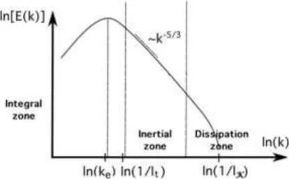
eddies, convected by the mean flow. Eddies strongly interact with each other through a cascade process which enhances the transfer of mass, momentum and heat compared to a laminar flow. The energetic density spectrum E(k) of the turbulent eddies in an homogeneous isotropic turbulence is displayed in Fig. 1.2 as a function of the wave number k proportional to the inverse of the eddy length scale.

Figure 1.2 - Sketch of energy density spectrum E(k) in an homogeneous isotropic turbulence. Distinction between integral, inertial and dissipation zones. The abscissa of the integral (lt) and

Kolmogorov (l_K) length scales are indicated [127].

Three different zones may be identified [127]:

• Integral zone: it is characterized by the lowest frequencies and it is centered on

the wave number ke. It contains the biggest and most energetic structures related

to the integral length scale lt, fixed by the production conditions of turbulence, and

to the turbulent speed up. The resolved turbulent kinetic energy k characterizing

this region is given by:

k = u ⇣2 i 2 = 3u2 p 2 , (1.39)

where upis the turbulent speed defined as the mean standard deviation of velocity.

The length scale and velocity of the integral zone structures are comparable to the quantities used to define the Reynolds number of the flow field and are not affected by viscous effects.

• Dissipation zone: it is characterized by the highest frequencies and it is centered

Kolmogorov scales which length lK and speed uK are estimated as [153]: l_K = , ν3 ⇧ -1/4 and uK =(ν⇧)1/4, (1.40)

where⇧ is the dissipation which converts the turbulent kinetic energy k into heat

due to the mixture kinematic viscosityν.

• Inertial zone: in this zone, the large eddies become unstable and break down into smaller eddies via a "cascade" process. No eddy dissipation is detected and the

energy is transfered from the biggest to the smallest structures following a k−5/3

law for isotropic steady turbulence.

1.2.1

Combustion regimes

Building a turbulent combustion model generally requires a classification of the differ-ent combustion regimes classically based on the characteristic dimensions of turbulence and chemistry. The chemical phenomena are characterized by the chemical time:

↵c=

⌅L

SL ,

(1.41)

where⌅Land SLare respectively the thickness and flame speed of a laminar premixed

flame.2 _{On the contrary, turbulent combustion involves very different lengths, velocities}

and times and the flame interacts at the same time with the most energetic turbulent

structures characterized by the turbulence time scale↵t =lt/up, and with the turbulence

smallest scales characterized by the Kolmogorov time scale↵_K =l_K/u_K:

• The characteristic turbulence time scale ↵tis compared to the chemical time scale

↵cvia the Damköhler number:

Da = ↵t ↵c = lt ⌅L SL up. (1.42)

For high Damköhler number Da>> 1, the internal thin structure of the flame is not

strongly affected by turbulence although the flame surface is wrinkled, stretched and convected by the turbulent flow. The reaction zone can be modeled by a laminar flame element named "flamelet". In the limit of small Damköhler number

Da << 1, reactants and products are mixed by turbulence before reacting via a

slow chemical reaction like in a perfectly stirred reactor. In pratical applications,

1.2 Turbulent premixed combustion

both regimes are usually found: fuel oxidation usually corresponds to a fast

chemical reaction (Da >> 1), whereas pollutant formation (CO oxidation or NO

formation) are slower.

• The Karlovitz number identifies the different interactions between turbulence small scales and flame:

Ka = ↵c ↵K = ⌅L l_K u_K SL . (1.43)

The relation SL↵ ν/⌅L[124] leads to a unity flame Reynolds number3:

Ref =

⌅LSL

ν ↵ 1. (1.44)

Using Eqs. (1.40) and (1.44) the Karlovitz number is rewritten as: Ka = $_u K SL 3/2,_l K ⌅L -−1/2 =$ ⌅L lK 2 . (1.45)

Thus, the Karlovitz number compares the flame length scale to the smallest tur-bulence structure.

Since the Reynolds, Damköhler and Karlovitz numbers are related through Re =

Da2_Ka2_{the transition between the different combustion regimes is completely defined}

by two of them (Fig. 1.3).

0.1 1 10 100 1000 u p / S L 0.1 1 10 100 1000 lt / δL Laminar flames Re=1 Ka_R=1(lk=δ_R) up=SL Reaction sheet Corrugated flamelets Wrinkled flamelets Well-stirred reactor Ka=1(lk=δL)

Figure 1.3 - Regime diagram for premixed turbulent combustion [117].

3_{From [173] and [90] the flame Reynolds number is usually assumed constant and approximately}

To distinguish the turbulence effects on the flame inner structure, i.e. the reaction zone, from the turbulence effect on the whole flame comprising also the preheating and the postflame zones, one additional Karlovitz number is defined using the reaction

zone thickness⌅r[117]: Kar = $⌅r lk 2 =$ ⌅r ⌅L 2$⌅ L lk 2 ↵ 1 100 $⌅l lk 2 ↵ Ka 100. (1.46)

Five different regimes have been defined by Peters [117] (Fig. 1.4):

• Laminar flame regime (Ret < 1): the flow is laminar and the flame is slightly

wrinkled.

• Wrinkled flamelet regime (Ret > 1, Ka < 1, up/SL < 1 ): when Ka < 1, the

flame thickness is smaller than the Kolmogorov scale. The flame element can be associated to a laminar flame and its surface is only slightly wrinkled by the

vortex passage due to up/SL < 1 (Fig. 1.4). The interaction between turbulence

and flame is limited.

• Corrugated flamelet regime (Ret > 1, Ka < 1, up/SL > 1 ): the flamelet regime

is still valid but, since up/SL > 1, the flame surface is more curved and stretched

with the formation of pockets of size similar to the eddy size.

• Reaction-sheet regime (Ret > 1, Ka > 1, Kar < 1 ): the smallest eddies of length

lk are smaller than the flame thickness⌅L(Ka > 1) and they can interact with the

preheat zone of the flame enhancing heat and mass transfers. The preheat zone is then thickened whereas the reaction zone, that is thinner than the Kolmogorov

length scale (Kar< 1), is not affected and keeps its laminar nature.

• Well-stirred reactor regime (Ret > 1, Ka > 1, Kar > 1 ): the Kolmogorov scale

lk is smaller than the reaction zone thickness⌅r (Kar > 1) and both preheat and

reaction zones are affected by turbulent motions. The smallest eddies penetrate into the reaction zone, increasing diffusion and heat transfer rate to the preheat zone. The flow behaves like a well-stirred reactor without any distinct laminar structure.

The distinction of the different combustion regimes based on the Reynolds and Karlovitz numbers is only qualitative since:

• the homogenous and isotropic turbulence is supposed unaffected by heat release, which is not true for combustion systems;

1.2 Turbulent premixed combustion

Figure 1.4 - Turbulent premixed combustion regimes illustrated in a case where the fresh and burnt gas temperatures are 300 and 2000 K respectively [124, 91].

• the entire analysis is based on order of magnitude estimations, i.e. the flamelet regime limit could correspond to Ka = 0.1 or Ka = 10 [31, 42];

• there is no experimental verification that eddies actually enter the flamelet and increase diffusivity [52];

• a one-step irreversible reaction chemistry has been assumed for this classification. Combustion is generally characterized by multiple species and reactions with consequently very different chemical time scales.

Most of combustion applications belong to the flamelet regime (Da >> 1). An

example of corrugated flame regime is the interaction between a pair of vortices and a flame analyzed in Section 4.1 whereas the reaction-sheet regime characterizes the flame interaction with a homogeneous isotropic turbulence (HIT) and the Bunsen flame studied in Sections 4.2 and 4.3 respectively.

1.2.2

Turbulent flame speed

In the flamelet regime, the turbulent flame front can be locally modeled by a laminar premixed flame which is stretched and deformed by turbulence.

The main effect of turbulence on combustion is the flame front wrinkling [15], by the

large turbulent scales, augmenting its effective area AT (Fig. 1.5).

Figure 1.5 - Sketch of the wrinkled area ATand of the mean flame surface AL. The flamelet consumption speed SCand the turbulent brush local consumption speed STare also labeled [52].

As a consequence, the rate of reactant consumption increases, augmenting the prop-agation speed of the mean front. For the flamelet regime, it is supposed that the front

locally propagates at the laminar velocity SL. The turbulent flame is then propagating

with a turbulent speed ST equal to the laminar flame speed weighted by the ratio of

the wrinkled instantaneous front area AT and the projected unwrinkled area AL[52]:

ST

SL

= AT

AL

I0, (1.47)

where I0 =SC/SLis the burning intensity defined as the ratio between the time average

of the flamelet consumption speed SCand the local laminar speed. The typical behavior

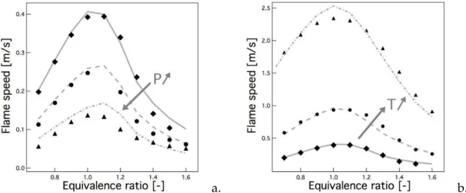
of the turbulent velocity ST/SLis represented in Fig. 1.6 as a function of up for various

pressures. The turbulent speed ST increases with the turbulence intensity as well as

with pressure. A gradually decreasing slope for high turbulence intensities is detected denoting that beyond a certain level the impact of turbulence intensity on turbulent flame is reduced.

1.2 Turbulent premixed combustion

Figure 1.6 - Experimental turbulent burning velocity as function of turbulence intensity and pressure for methane-air mixture at equivalence ratioφ = 0.9 [89]. The investigated pressure values are

P = 0.1, 0.5, 1.0, 2.0, 3.0 MPa.

1.2.3

Combustion modelling for LES

Different models have been proposed to approximate the filtered species reaction rates ˙

ωk for turbulent premixed combustion of Eq.(1.35) using the LES approach [76, 10].

They may be separated into two main categories:

• Models assuming an infinitely thin reaction zone: the turbulent premixed flame is modeled by fresh reactants and burnt products separated by an infinitely thin reaction zone. The local structure of the flame is assumed equal to a laminar flame for which the inner structure is not affected by turbulence (flamelet as-sumption). The Bray-Moss-Libby (BML) models [28], the flame surface density models [74, 108], the flame wrinkling description [170] and G-equation mod-els [117, 53, 119, 112] are some of the most common examples.

In the BML model, the progress variable c(x, t) is the only quantity defining the thermochemical state of the mixture. All other mean quantities are described in terms of a probability density function P(c, x) which represents fresh reactants,

burnt products and a partially burned mixture with probabilityα(x), ⇥(x) and ⇤(x)

respectively, where_{⇤(x) ' 1. The mean values of quantities such as species mass}

fractions only depend onα(x) and ⇥(x).

In the coherent flamelet model (or flame surface density model) the mean chem-ical reaction rate is expressed in terms of the flame surface density where con-ditions are favorable for reaction. The balance equation required for the flame surface density accounts for average stretch rate and extinction.

In the level set approach (or G-equation approach), a function G(x, t) is defined

are found and the fresh reactants are located where G< G0. A transport equation is solved for the function G(x, t) based on kinematic considerations.

• Models describing the reaction zone thickness: the turbulent premixed flame is characterized by a finite thin reaction zone that could interact with the turbulent flow and often behaves as a stretched laminar flame. Some examples are the Probability Density Function (PDF) models [6, 51] and the artificially thickened flame (TF) models [8, 7, 93].

In the Probability Density Function model, mean values and correlations of quantities of interest are extracted by the use of a probability density function, based on statistical properties of a scalar field such as the progress variable c. The artificially thickened flame approach is the one used in this study and is detailed below.

Artificially thickened flame model for LES (TFLES)

The flame thickness ⌅L is usually smaller than the LES filter size ∆. The artificially

thickened flame approach for LES (TFLES) has been proposed in order to resolve the flame front on a LES grid [8, 7, 93].

The whole TFLES method is based on a simple change of the spatial and temporal variables:

x◆→ F x and t ◆→ F t, (1.48)

which corresponds to a thickening of the flame thickness by a factor _{F . The filtered}

species and thermal reaction rates are: ˙ ωk = ˙ ωk F and ω˙T = ˙ ωT F . (1.49)

Following the theory of laminar premixed flames [173], the flame speed SL is

conse-quently modified: SL⇧ Dth ⌅L ◆→ Dth F ⌅L. (1.50) In order to maintain the same flame speed, the thermal and species diffusivities are also multiplied by F: Dth◆→ F Dth and Dk ◆→ F Dk, (1.51) so that SL◆→ F Dth F ⌅L = Dth ⌅L . (1.52)

1.2 Turbulent premixed combustion Mass fraction [-] 12x10-3 11 10 9 8 7 6 5 x [mm] Product Reactant a. 4x109 3 2 1 0 Heat release [J/m3/s] 12x10-3 11 10 9 8 7 6 5 x [m] _b.

Figure 1.7 - Results for a flame thickened by a factorF = 4 (lines) compared to the reference solution of a laminar unthickened flame (symbols).

Results for a laminar premixed flame are shown in Fig. 1.7 using a thickening factor F = 4. The gradient profiles are decreased allowing the use of a coarse grid. The

maximum values of reaction rates and heat release are reduced by a factor _{F = 4.}

However, the integrals of reaction rates are conserved and consequently the laminar flame speed is conserved too.

When a turbulent flame is artificially thickened, the flame front is less wrinkled by the turbulent eddies and the time scale ratio between turbulence and chemistry is

modified. The so-called efficiency function _{E [46, 36] has been proposed to properly}

account for the wrinkling effect on the flame front:

Dth ◆→ EF Dth and Dk ◆→ EF Dk (1.53) ˙ ωk = E ˙ ωk F and ω˙T = E ˙ ωT F , (1.54) so that: SL◆→ EF Dth F ⌅L =ST. (1.55)

This model has been first developed for perfectly premixed combustion. The imple-mentation of the TFLES method in a numerical code and its extention to partially premixed combustion and multi-reactions chemistries are presented in Chapter 3.

1.3

Chemistry for turbulent combustion

Chemical kinetic models are used to describe the transformation of reactants into prod-ucts at the molecular level. Different detailed mechanisms characterizing the combus-tion phenomena of alkanes, alkynes and aromatics species are available [148]. These mechanisms characterized by hundreds of species and thousands of reaction are sup-posed to accurately and reliably describe all kinds of combustion phenomena over all possible ranges of the thermodynamic parameters such as pressure, initial composition and temperature. Nevertheless, this kind of mechanism is computationally expensive due to the large number of species and reactions. Moreover, numerical problems of-ten occur when solving the stiff system of conservation equations involving different chemical time scales [91] (Fig. 1.8). For these reasons, different methods of mechanism reduction have been developed.

Figure 1.8 - Range of chemical time scales [166].

In this section, different approaches to approximate the species reaction rates ˙ωk

defined in Eq. (1.8) are presented:

• mechanism reduction by elimination of redundant species and reactions (skeletal and reduced mechanisms);

• dimension reduction of the phase space by the generation of a lower-dimensional

manifold involving only P < N parameters, N being the number of species. The

thermochemical system generally evolves in a space of 2+N dimension (pressure, enthalpy and mass fraction of N species), but follows much lower-dimensional paths in this phase-space.