Portfolio Methods in Uncertain Contexts

HAL Id: tel-01250552

https://tel.archives-ouvertes.fr/tel-01250552v2

HAL is a multi-disciplinary open access

archive for the deposit and dissemination of sci-entific research documents, whether they are pub-lished or not. The documents may come from

L’archive ouverte pluridisciplinaire HAL, est destinée au dépôt et à la diffusion de documents scientifiques de niveau recherche, publiés ou non, émanant des établissements d’enseignement et de

Portfolio Methods in Uncertain Contexts

Jialin Liu

To cite this version:

Jialin Liu. Portfolio Methods in Uncertain Contexts. Artificial Intelligence [cs.AI]. Université Paris Saclay (COmUE), 2015. English. �NNT : 2015SACLS220�. �tel-01250552v2�

T

HÈSE

DE

DOCTORAT

DE

L’U

NIVERSITÉ

P

ARIS

-S

ACLAY

PRÉPARÉE

À

L

'U

NIVERSITÉ

P

ARIS

-S

UD

I

S

L

E

D

° 580

Sciences et technologies de l'information et de la communication

Spécialité Informatique

Par

Mlle. Jialin Liu

Portfolio Methods in Uncertain Contexts

Thèse présentée et soutenue à Orsay, le 11 décembre 2015:

Composition du Jury :

M. Dague, Philippe Professeur, Univ. Paris-Saclay Président M. Bouzy, Bruno MDC, Univ. Paris Descartes Rapporteur M. Gallagher, Marcus MDC, Univ. of Queensland Rapporteur M. Lucas, Simon Professeur, Univ. of Essex Examinateur M. Posik, Petr Professeur, Gerstner Laboratory Examinateur M. Rudolph, Günter Professeur, Univ. of Dortmund Examinateur

Acknowledgments

First and above all, I would like to express my gratitude to my advisors, Dr. Olivier Teytaud and Dr. Marc Schoenauer, for the continuous support of my Ph.D research, their patience, their warm encouragement, excellent guidance and immense knowledge. Olivier is always reflective, astute and continuously available for helping me. Olivier and his wife Maud, who encouraged me when I was down, are more like my friends, and sometimes as big brother and big sister. I’ll forever remember the word Marc has comforted me when I made mistakes: “Il n’y a que ceux qui ne font rien qui ne font jamais d’erreur”.

Besides my advisors, I would like to thank Prof. Philippe Dague, for offering me the opportunity to come to France for my master study on 2009, then being the president of the jury. Many thanks to Prof. Bruno Bouzy and Prof. Marcus Gallagher who accorded me the great honour of accepting to review my work and for their great comments and appreciation of our work. I would like also thank Prof. Simon Lucas, Dr. G¨unter Rudolph and Prof. Petr Posik for being in my committee and providing valuable feed-back.

My deepest gratitude also goes to all the members of TAO team and Artelys, who have provided a warm and comfortable research environment. A special mention to Sandra and Marie-Liesse, with whom I learnt a lot of math; to Jean-Baptiste, Vin-cent and Jérémie, real geeks; to Adrien, for all his advices; to Gaéten, who provided a relexed office environment; to Nicolas, for the laughs he brought; to Yann, Fabrice and Peio, who received me warmly in Artelys.

Thanks to all members of AILab team of National Dong Hwa University for their kindly help when we visited Taiwan.

Many thanks to the administrative staff of INRIA and the Université Paris-Saclay and, in particular, Mrs. Valérie Berthou, Mrs. Stéphanie Druetta, Mrs. Marie-Carol Lopes and Mrs. Olga Mwana-Mobulakani, for their help, careful work and patience.

My sincere thanks also go to Prof. Emmanuelle Frenoux and Dr. Agnes Pailloux, for their help and recommendations. I thank Prof. Jérôme Azé, who brought me to Computer Science and

Bin, for offering valuable advice, for their support as my friends and families during the whole period of the study. A lot of thanks to Yi, my dear friend. For the last ten years, we have been achiev-ing our aims and dreams step-by-step.

I warmly thank and appreciate my father, Prof. Yamin Liu, for his support in all aspects of my life. I also would like to thank my mother, Mrs. Luopei Zhang. For years she has kept on trying to stop me continuing my studies and research. Her continuous action reminds me everyday one of the most important elements of success both in research and life, that is perseverance.

Abstract

This manuscript concentrates in studying methods to handle the noise, including using resampling methods to improve the con-vergence rates and applying portfolio methods to cases with uncer-tainties (games, and noisy optimization in continuous domains).

Part I will introduce the manuscript, then review the state of the art in noisy optimization, portfolio algorithm, multi-armed bandit algorithms and games.

Part II concentrates on the work on noisy optimization: • Chapter 4 provides a generic algorithm for noisy

optimiza-tion recovering most of the existing bounds in one single noisy optimization algorithm.

• Chapter 5 applies different resampling rules in evolution strate-gies for noisy optimization, without the assumption of vari-ance vanishing in the neighborhood of the optimum, and shows mathematically log-log convergence results and stud-ies experimentally the slope of this convergence.

• Chapter 6 compares resampling rules used in the differen-tial evolution algorithm for strongly noisy optimization. By mathematical analysis, a new rule is designed for choosing the number of resamplings, as a function of the dimension, and validate its efficiency compared to existing heuristics -though there is no clear improvement over other empirically derived rules.

• Chapter 7 applies “common random numbers”, also known as pairing, to an intermediate case between black-box and white-box cases for improving the convergence.

Part III is devoted to portfolio in adversarial problems:

• Nash equilibria are cases in which combining pure strategies is necessary for designing optimal strategies. Two chapters are dedicated to the computation of Nash equilibria:

cally, we get improved rates when the support of the Nash equilibrium is small.

– Chapter 10 applies these results to a power system problem. This compares several bandit algorithms for Nash equilibria, defines parameter-free bandit algorithms, and shows the relevance of the sparsity approach dis-cussed in Chapter 9.

• Then, two chapters are dedicated to portfolios of game meth-ods:

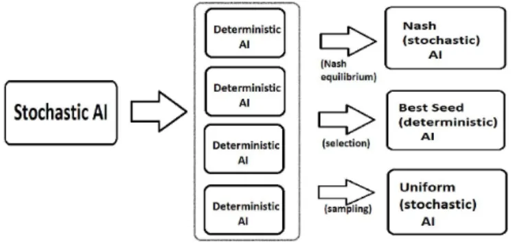
– Chapter 11 shows how to generate multiple policies, from a single one, when only one such policy is avail-able. This kind of bootstrap (based on random seeds) generates many deterministic policies, and then com-bines them into one better policy. This has been tested on several games.

– Chapter 12 extends chapter 11 by combining policies in a position-specific manner. In particular, we get a better asymptotic behavior than MCTS.

Part IV is devoted to portfolios in noisy optimization:

• Chapter 14 is devoted to portfolio of noisy optimization methods in continuous domains.

• Chapter 15 proposed differential evolution as a tool for non-stationary bandit problems.

5

Contents

I Introduction

15

2 State of the art 25

II Contributions in noisy optimization

63

3 Contributions to noisy optimization: outline 65 4 Resampling in continuous noisy optimization 67 5 Resampling in evolution strategies 81 6 Resampling in differential evolution 103 7 Grey box noisy optimization 123

IIIContributions in adversarial portfolios

135

9 Sparse Nash equilibria 139 10 Nash-planning for scenario-based decision making 157

11 Optimizing random seeds 171

12 Optimizing position-specific random seeds: Tsumegos 189

IVPortfolios and noisy optimization

207

13 Portfolios and noisy optimization: outline 209 14 Portfolio of noisy optimization methods 211 15 Differential evolution as a non-stationary portfolio method237

V Conclusion and Perspectives

255

16 Overview and conclusion 257

17 Further work 261

Noisy optimization algorithms 262

Summary of notations 262

Acronyms 266

List of Figures 270

Contents (detailed) Bibliography 275

Contents (detailed)

I Introduction

15

1.2 Biological intelligence versus computational intelli-gence . . . 20

1.2.1 Emotions and portfolios . . . 21

1.2.2 Is the emotion a harmful noise ? . . . 21

1.2.3 Portfolios in practice . . . 22

1.3 Application fields in this thesis . . . 22

2 State of the art 25 2.1 Noisy Optimization . . . 26

2.1.1 Framework . . . 27

2.1.2 Local noisy optimization . . . 30

2.1.3 Black-box noisy optimization . . . 31

2.1.4 Optimization criteria . . . 32

2.1.5 Motivation and key ideas . . . 35

2.1.6 Resampling methods . . . 37

2.2 Portfolio Algorithms . . . 43

2.2.2 Applications of portfolio algorithms . . . 46

2.3 Multi-Armed Bandit . . . 46

2.3.1 Multi-armed bandit framework and notations 47 2.3.2 Sequential bandit setting . . . 47

2.3.3 Algorithms for cumulative regret . . . 48

2.3.4 Adversarial bandit and pure exploration ban-dit . . . 51

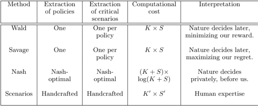
2.4 Scenario-Based Decision-Making . . . 52

2.4.1 Decision making in uncertain environments . 52 2.4.2 State of the art: decision with uncertainties 53 2.4.3 Comparison between various decision tools . 56 2.5 Games . . . 56

2.5.1 AIs for games: the fully observable case . . . 56

2.5.2 Improving AI: endgames and opening books 58 2.5.3 Partial Observation and Nash Equilibria . . 58

II Contributions in noisy optimization

63

4.1.2 Examples of algorithms verifying the LSE assumption . . . 70

4.2 Convergence Rates of Inoa . . . 75

4.2.1 Rates for various noise models . . . 75

4.2.2 Application: the general case . . . 76

4.2.3 Application: the smooth case . . . 76

4.3 Conclusion and further work . . . 77

5 Resampling in evolution strategies 81 5.1 Theoretical analysis: exponential non-adaptive rules can lead to log/log convergence. . . 83

5.1.1 Preliminary: noise-free case . . . 83

5.1.2 Scale invariant case, with exponential num-ber of resamplings . . . 84

Contents (detailed) 5.1.3 Extension: adaptive resamplings and

remov-ing the scale invariance assumption . . . 87

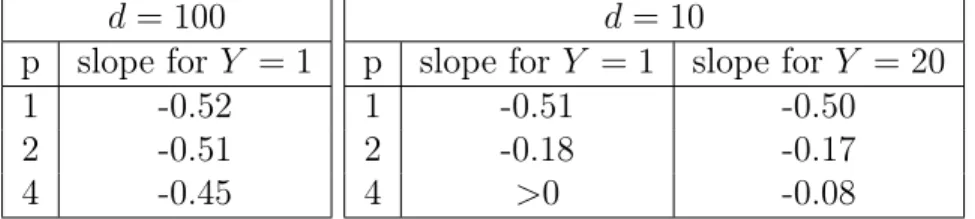
5.2 Polynomial number of resamplings: experiments . . 88

5.3 Experiments with adaptivity: Y ⌘ n revaluations . . 89

5.4 Comparison of resampling rules for Evolutionary Noisy Optimization on a Unimodal Function . . . . 91

5.4.1 Experimental setup . . . 92

5.4.2 Experiments with polynomial number of re-samplings . . . 92

5.4.3 Experiments with exponential number of re-samplings . . . 93

5.4.4 Experiments with resampling number depend-ing on d and n . . . 98

5.4.5 Discussion and conclusion: choosing a non-adaptive resampling rule . . . 98

5.5 Conclusion: which resampling number in noisy evo-lution strategies ? . . . 100

5.5.1 What is a good noisy optimization algorithm?100 5.5.2 Overview of our results . . . 101

6 Resampling in differential evolution 103 6.1 Differential evolution & noisy differential evolution 103 6.1.1 Differential evolution . . . 103

6.1.2 Noisy differential evolution: state of the art 105 6.1.3 Non-adaptive and adaptive noisy differential evolution . . . 106

6.2 Experiments . . . 109

6.2.1 The CEC 2005 testbed . . . 109

6.2.2 Parameter selection for DE on the CEC 2005 testbed . . . 110

6.2.3 Adding strong noise in the CEC 2005 testbed 110 6.2.4 Experimental results . . . 111

6.3 Discussion & conclusions . . . 120

6.3.1 Main observations . . . 120

6.3.2 Special cases . . . 120

6.3.3 Conclusion: resampling in differential evo-lution . . . 120

7 Grey box noisy optimization 123

7.1 Grey box noisy optimization . . . 123

7.2 Algorithms . . . 123

7.2.1 Different forms of pairing . . . 123

7.2.2 Why common random numbers can be detri-mental . . . 124

7.2.3 Proposed intermediate algorithm . . . 125

7.3 Artificial experiments . . . 126

7.3.1 Artificial testbed for paired noisy optimization126 7.3.2 Experimental results . . . 127

7.4 Real world experiments . . . 128

7.4.1 Paired noisy optimization for dynamic prob-lems . . . 128

7.4.2 Unit commitment problem . . . 130

7.4.3 Testbed . . . 130

7.5 Conclusions: common random numbers usually work but there are dramatic exceptions . . . 132

IIIContributions in adversarial portfolios

135

9.1.1 Rounded bandits. . . 139

9.2 Analysis . . . 141

9.2.1 Terminology . . . 141

9.2.2 Supports of Nash equilibria . . . 142

9.2.3 Denominators of Nash equilibria . . . 144

9.2.4 Stability of Nash equilibria . . . 145

9.2.5 Application to sparse bandit algorithms . . . 149

9.3 Experiments . . . 150

9.4 Conclusion: sparsity makes the computation of Nash equilibria faster . . . 152

10 Nash-planning for scenario-based decision making 157 10.1 Our proposal: NashUncertaintyDecision . . . 158

Contents (detailed) 10.1.1 The algorithmic technology under the hood:

computing Nash equilibria with adversarial

bandit algorithms . . . 158

10.1.2 Another ingredient under the hood: sparsity 161 10.1.3 Overview of our method . . . 161

10.2 Experiments . . . 162

10.2.1 Power investment problem . . . 162

10.2.2 A modified power investment problem . . . 166

10.3 Conclusion: Nash-methods have computational and modeling advantages for decision making under un-certainties . . . 169

11 Optimizing random seeds 171 11.1 Introduction: portfolios of random seeds . . . 171

11.1.1 The impact of random seeds . . . 171

11.1.2 Related work . . . 171

11.1.3 Outline of the present chapter . . . 172

11.2 Algorithms for boosting an AI using random seeds . 173 11.2.1 Context . . . 173

11.2.2 Creating a probability distribution on ran-dom seeds . . . 174

11.2.3 Matrix construction . . . 174

11.2.4 Boosted AIs . . . 174

11.3 Rectangular algorithms . . . 175

11.3.1 Hoeffding’s bound: why we use K 6= Kt . . . 175

11.3.2 Rectangular algorithms: K 6= Kt . . . 176

11.4 Testbeds . . . 176

11.4.1 The Domineering Game . . . 177

11.4.2 Breakthrough . . . 177 11.4.3 Atari-Go . . . 178 11.5 Experiments . . . 179 11.5.1 Criteria . . . 179 11.5.2 Experimental setup . . . 179 11.5.3 Results . . . 179

11.6 Experiments with transfer . . . 183

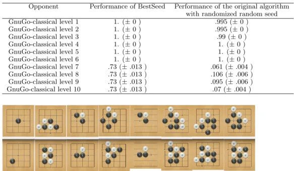
11.6.1 Transfer to GnuGo . . . 183

11.6.2 Transfer: validation by a MCTS with long thinking time . . . 184

11.6.3 Transfer: human analysis . . . 185

11.7 Conclusions: optimizing the seed works well for many games on small boards . . . 186

12 Optimizing position-specific random seeds: Tsumegos 189 12.1 Problem Statement . . . 189

12.1.1 Tsumego Problems . . . 189

12.1.2 Game Value Evaluation . . . 192

12.1.3 Weighted Monte Carlo . . . 193

12.2 Proposed algorithm and mathematical proof . . . . 194

12.2.1 Construction of an associated matrix game . 194 12.2.2 Nash Equilibria for matrix games . . . 195

12.2.3 Mathematical analysis . . . 196

12.3 Experiments on Tsumego . . . 198

12.3.1 Oiotoshi - oiotoshi with ko . . . 199

12.3.2 Seki & Snapback . . . 200

12.3.3 Kill . . . 200

12.3.4 Life . . . 201

12.3.5 Semeai . . . 201

12.3.6 Discussion . . . 201

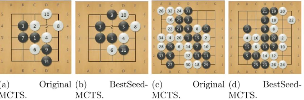
12.4 Conclusion: weighted MCTS has a better scalabil-ity than MCTS . . . 204

IVPortfolios and noisy optimization

207

14.2 Algorithms and analysis . . . 211

14.2.1 Notations . . . 211

14.2.2 Definitions and Criteria . . . 212

14.2.3 Portfolio algorithms . . . 214

14.2.4 Theoretical analysis . . . 216

14.3 Experimental results . . . 223 14.3.1 Real world constraints & introducing sharing 223

Contents (detailed) 14.3.2 Experiments with different solvers in the

port-folio . . . 225

14.3.3 The lag: experiments with different variants of Fabian’s algorithm . . . 230

14.3.4 Discussion of experimental results . . . 232

14.4 Conclusion: INOPA is a mathematically proved and empirically good portfolio method for black-box noisy optimization, and our simple sharing tests did not provide clear improvements . . . 232

15 Differential evolution as a non-stationary portfolio method237 15.1 Introduction . . . 237

15.2 Problem Statement . . . 239

15.2.1 Non-Stationary Bandit Problem . . . 239

15.2.2 Differential Evolution Algorithm . . . 241

15.2.3 Truncation . . . 242

15.2.4 Experiments . . . 243

15.2.5 Conclusion: UCBdn is preferable for small budget, truncated-DE is recommended for huge budget . . . 250

V Conclusion and Perspectives

255

16.2 Conclusions in noisy optimization by portfolio meth-ods . . . 257

16.3 Conclusions on computing Nash equilibria . . . 258

16.3.1 Conclusions on the modeling of decision un-der uncertainty thanks to Nash equilibria . . 258

16.3.2 Conclusions on the computational aspects of Nash equilibria . . . 259

16.4 Contribution in portfolio methods for adversarial problems. . . 259

Noisy optimization algorithms 262 Summary of notations 262 Acronyms 266 List of Figures 270 List of Tables 272 Bibliography 275

Part I

Contents (detailed) 17

Disclaimer

M.-L. Cauwet had a strong contribution to the theoretical part of the work on portfolio [Cauwet et al., 2014] and of the work on noisy optimization in continuous domains [Astest Morales et al., ]; S. Astete-Morales also contributed to this continuous noisy op-timization work [Astest Morales et al., ]. B. Rozière contributed to the portfolio work, for the INOPA part [Cauwet et al., 2014]. I am the author of the experimental works in Tables 14.1, 14.2, 14.3, 14.4 and 14.5. S. Astete-Morales contributed to the work on resamplings in continuous optimization [Astete-Morales et al., 2013]. We collaborated for the theory and I am the author of experimental results in Figures 5.2, 5.3, 5.4 and 5.5. J. Decock contributed to the work on grey-box noisy optimization [Decock et al., 2015], Chapter 7. I am the author of results in Tables 7.1 and 7.2. J. Decock is the author of the results in Figures 7.1. I am, with my ph.D. advisor O. Teytaud, the author of the papers used for Chapters 5, 9, 11 and 14. I used some codes from Na-tional Dong Hwa University (Hualien), AILAB team, for the work on noisy optimization with differential evolution.

Two strong amateur go players, S.-J. Yen from AILAB team and K.-H. Yeh from National Chiao-Tung University (Hsinchu), have played with our modified version of GnuGo (Figure 11.10).

19

1 Motivation

1.1 Big news in AI

There are recently quite a lot of big news in AI, including an impact in general audience newspapers:

• Deep learning: how far from human performance (in terms of image recognition)? Deep learning provides great per-formance in image recognition, outperforming existing algo-rithms; it also performs surprisingly well for recognizing good moves on a Go board. Recently, a chess engine called Giraffe, which uses a neural network for training, was announced to play at approximately International Master Level [Lai, 2015]. However, improvement is always necessary.

• There is also a strong progress in domains in which com-puters have been widely used for dozens of years, such as numerical optimization. In particular, portfolio methods are essential components for successful combinatorial optimiza-tion. On 2007, SATzilla [Xu et al., 2008], which uses em-pirical hardness models to choose among their constituent solvers, got an excellent performance (three gold, one silver and one bronze medal) in the SAT Competition1_{. In this}

thesis, we will focus on portfolio methods and in particular their application in uncertain settings.

• Another example can be found in games. Monte Carlo Tree Search (MCTS) provided the best algorithm for the game of

Go, outperforming alpha-beta by far, and is now routinely used in many difficult games. MoGo [Lee et al., 2009]2 _made

the first wins against professionals in 9x9 and with large handicap in 19x19; nowadays, there are strong programs such as Zen and CrazeStone who can win against top play-ers with handicap 5. During the Human vs. Computer Go Competition at CIG20153_{, Aya won against a 9P player with}

handicap 5 in 19x19.

MoGo is empirically close to perfect play in 7x7. Still, in spite of various great successes in Go and in other games, there are unsolved issues in MCTS, and in particular scal-ability issues, i.e. a plateau in performance when the num-ber of simulations becomes large. We will propose weighted Monte Carlo Tree Search, which outperformed Monte Carlo Tree Search on a family of Tsumego problems.

1.2 Biological intelligence versus computational

intelligence

One of the lessons from noisy optimization is that the best conver-gence rates are obtained when we use sampling all over the domain, and not only close to the approximate optimum; this is the key for the difference between simple regret decreasing as the inverse of the number of evaluations, instead of as the square root of the inverse of the number of evaluations [Fabian, 1967,Astest Morales et al., ]. It is known that nature contains random exploration, for kids mainly; this is a (late) justification for large mutations. We here discuss a different, less well known, inspiration from biology: emotions as a (biological) tool for portfolios.

2_{https://www.lri.fr/~teytaud/mogo.html.}

3_{2015 IEEE Conference on Computational Intelligence and Games, http:}

1.2. Biological intelligence versus computational intelligence

1.2.1 Emotions and portfolios

Emotion is a key difference between human beings and machines. (The physical differences such as blood, cells are out of my area of interest, yet what need to be mentioned is that Neural networks are already a common tool in AI.) For an agent, the lack of emotion is ambiguous as the emotion can be sometimes regarded as noise for human beings. However, emotion can also trigger a choice between several kinds of behaviors: it is known that, in case of fear, humans have more power in legs (for running away) and arms (for attacking); we are somehow in a portfolio method. Also, for preserving equilibrium, there are several methods available in the brain, and different people prefer different methods (using more or less visual stimuli). When several methods are available, they are termed “vicariant processes”, and animals/humans can choose between several of them [Reuchlin, 1978].

1.2.2 Is the emotion a harmful noise ?

The emotion is often unneglected but difficult to be modelized. Besides, it cannot be arbitrarily considered as a harmful noise. For instance, little white lies may be far more innocuous in real life; AI may make optimal choice but not reasonable or friendly choice. The real “intelligence” can not be achieved by an AI with-out emotion. AI may learn the emotion by words, tone analyze, facial recognition and brainwave detection. Recently, IBM has proposed a service called “IBM Watson Tone Analyzer” to detect emotional tones4_{. Regardless of its performance, there is still}

un-solved question: can AI simulate emotion and make decisions with emotion? On 2009, Henry Markram, director of the “Blue Brain Project”, has claimed that a functional artificial human brain can be built within the next 10 years. However, the reality is not very optimistic. The idea is plump, however, the reality is scrawny, says a Chinese proverb.

4_{https://developer.ibm.com/watson/blog/2015/07/16/}

1.2.3 Portfolios in practice

There are a large number of state-of-the-art black-box continuous noisy optimization algorithms, which have their own specialization and are dominant in some different particular frameworks. In real life, however, the situation is more complicated and unstable. The choice of algorithms is thus not trivial. It makes sense to com-bine the existing algorithms rather than defining new algorithms. A classical application is Combinatorial Optimization in discrete domains.

We propose in this manuscript two novel applications for port-folio methods:

• Noisy Optimization in continuous domains, where the com-parison of two similar solutions is more expensive than their determinations. This difference cannot be neglected. This is our main motivation of working on algorithm portfolios for noisy optimization, which chooses online between several algorithms.

• Games, using the concept of Nash Equilibrium, where non mono-selection is made, but some combinations of strategies are recommended.

These two applications have been performed on both games and electrical systems.

By creating multiple strategies based on the perturbation and combination of random seeds, our method outperforms a standard MCTS implementation in Go, for large numbers of simulations, without computational overhead.

1.3 Application fields in this thesis

The main application fields of this thesis are games and electrical systems. In electrical systems, the transition of energy is a main issue due to some stochastic effects such as faults, climate changes, oil resources, political and geopolitical problems, technology devel-opments and accidents, such as post-Fukushima. The stochasticity

1.3. Application fields in this thesis also increases as renewable energy increases. In the traditional

op-timization of energy systems, disappointingly, the noise is usually badly treated by deterministic management. This leads us to ap-ply noisy optimization to energy systems. The robustness is much more important than the precision in energy problems, therefore, we prefer to spend more evaluations (computational time) to make a better choice.

Another interesting question, emerging by comparing power systems and games, is as follows: shall we propose a probability distribution of strategies to some electricity companies in order to make a choice according to the distribution? A key point is that some decision criteria naturally lead to stochastic decisions (mixed Nash equilibria), as in games. That’s a gambling for high stakes. This inspires us to work on some robust decision making approaches.

25

Artificial intelligence is the art of automatic decision making. Decisions can be made in various settings:

• We have a function f (termed objective function) which quantifies the quality of a decision; then, we look for a deci-sion x such that f(x) is optimal. This is termed optimiza-tion.

• We have such a function f, but its results are noisy; we wish to find an x such that f(x) is optimal on average. This is termed noisy optimization.

• The function f can only be applied to a remote state. The decision to be made has an impact later; i.e., the reward is delayed, and possibly depends on other later decisions, from us, but also, possibly, from other persons (termed agents). This is termed control or reinforcement learning when there is no other agent than us, and games when several agents are concerned.

In this manuscript, we will work on noisy optimization and games. The central tool is the use of portfolio methods; rather than defining new methods, we combine existing ones. As port-folio methods are already a well established domain in noise-free optimization, we focus on cases with uncertainties, such as noisy optimization, and adversarial problems, such as games.

2.1 Noisy Optimization

The term Noisy Optimization refers to the search for the optimum of a given stochastic objective function f : (x, w) 7! f(x, w) where x is in the search domain D 2 Rd _{and w is some random}

pro-cess. From now on, we assume the existence of some x⇤ _{such that}

Ewf (x⇤, w) is minimum. Many results regarding the performance

of algorithms at solving these problems and at the complexity of the problems themselves have been developed in the past, always trying to broaden the extent of them. In this manuscript we pro-pose an optimization algorithm that allows us to generalize results in the literature as well as providing proofs for conjectured results.

2.1. Noisy Optimization We start by stating shortly the framework and definitions of the concepts we will review. Then we comment the state of the art related to stochastic optimization, which will bring us to the specific motivation of this manuscript. We finish this section with an outline of the reminder of the work.

2.1.1 Framework

When the gradient is available for the optimization process, there are algorithms developed in the literature that show a good per-formance: moderate numbers of function evaluations and good precision. Such is the case for Stochastic Gradient Descent, which is the stochastic version of the classic Gradient Descent Algorithm. Nonetheless, having access to a gradient is a major assumption in real life scenario. Therefore, in this manuscript, we focus on a black-box case, i.e. we do not use any internal property of f, we only have access to function evaluations for points in the search space - and, in some cases, a slightly grey box scenario (using random seeds).

A noisy black-box optimization algorithm at iteration m 1: (i) chooses a new point xm in the domain and computes its

objec-tive function value ym = f (xm, wm), where the wmare independent

copies of w; (ii) computes an approximation ˜xm of the unknown

optimum x⇤_.

Therefore, at the end of the application of the noisy optimiza-tion algorithm, we obtain several sequences: the search points (xm)m 1, the function value on the search points (ym)m 1 and the

approximations (˜xm)m 1. Let us note that each search point xm

is a computable function of the previous search point and their respective function values. But the computation of the search point involves random processes: the stochasticity of the function, and/or some specific random process of the algorithm, if the latter is randomized. The point ˜xm is termed recommendation, and it

represents the current approximation of x⇤_{, chosen by the}

algo-rithm. Even though in many cases, the recommendation and the search points are exactly the same, we will make a difference here because in the noisy case it is known that algorithms which do not

distinguish recommendations and search points can lead to poor results1_{, depending on the noise level.}

It is necessary to state a merely technical comment, related to the indexation of the sequences mentioned above and the exact notation used in this manuscript. Depending on the study that one is carrying, there are arguments for indexing the sequences by iterations or by function evaluations. It occurs often in the case of optimization of noisy functions, that it is more convenient to have multiple evaluations per iteration. Therefore, the best idea is to keep the iteration index, rather than indexing the sequences by the number of evaluations. We will then use xm,1, . . . , xm,rm to

denote the rm search points2 at iteration m. On the other hand,

xopt_m , with only one subscript, is the recommended point at iteration m.

For consistency in criteria in the following sections, ˜xn will

always denote the recommendation after n evaluations. Hence, when the approximations of the optimum are defined per iteration rather than per evaluation, the sequence of recommended points is redefined as follows, for all n 1: ˜xn = xoptk , where k is maximal

such thatPk 1

i=1 ri  n.

Now that we have defined the basic notations for the algorithms considered in this work, let us introduce the optimization criteria which will evaluate the performance of the algorithms. They al-low us to compare the performance of the algorithm considering all search points or only the recommended points. The informa-tion we have on the cost of evaluating search points can be the dealbreaker when choosing what algorithm to use, as long as we have specialized optimization criteria to help us decide. We will consider three criteria: Uniform Rate (UR), Simple Regret (SR) and Cumulative Regret (CR), respectively defined in Equations 2.1, 2.2 and 2.3.

1_{See [Fabian, 1967, Coulom, 2012] for more on this.}

2_{When we need to access to the m}th_{evaluated search point, we define x}0 m

the mth _{evaluated search point, i.e. x}0

m = xi,k with m = Pi 1j=1rj + k and

2.1. Noisy Optimization

s(U R) = lim sup

i log(U Ri) log(i) (2.1) s(SR) = lim sup i log(SRi) log(i) (2.2) s(CR) = lim sup i log(CRi) log(i) (2.3)

where URi is the 1 quantile of kx0i x⇤k, SRi is the 1

quantile of Ewf (˜xi, w) Ewf (x⇤, w), CRi is the 1 quantile

of Pji Ewf (x0j, w) Ewf (x⇤, w) . k.k stands for the Euclidean

norm, x0

i denotes the ith evaluated search point and ˜xi denotes

the recommendation after i evaluations. We have expectation op-erators Ew above with respect to w only, therefore Ewf (˜xi, w) is

not deterministic. Quantiles Q1 are with respect to all

remain-ing stochastic parts such as noise in earlier fitness evaluations and possibly internal randomness of the optimization algorithm.

In Equations 2.1, 2.2 and 2.3, we consider the slopes in log-log graphs (x-axis: log of evaluation numbers; y-axis: log of UR or SRor CR). The use of the slopes turns out to be more convenient because it allow us to know with one single number how fast an algorithm is reaching the specific optimization criterion.

These quantities depend on the threshold , but in all cases below we get the same result independently of , therefore we will drop this dependency.

Note that, for s(UR) and s(SR), 0 can be trivially reached by an algorithm with constant (x0

m, ˜xm). Therefore, s(UR) and

s(SR) are only interesting when they are less than 0. And s(CR) is relevant when it is less than 1.

Finally, regarding to the objective functions, we investigate three types of noise models :

V ar(f (x, w)) = O ([Ewf (x, w) Ewf (x⇤, w)]z) z 2 {0, 1, 2}

(2.4) We will refer to them respectively as the case where the variance of the noise is constant, linear and quadratic as a function of the simple regret.

2.1.2 Local noisy optimization

Local noisy optimization refers to the optimization of an objective function in which the main problem is noise, and not local minima. Hence, diversity mechanisms as in [Jones et al., 1998] or [Auger et al., 2005], in spite of their qualities, are not relevant in this manuscript. We also restrict our work to noisy settings in which noise may not decrease to 0 around the optimum. This constrain makes our work different from [Jebalia et al., 2010]. In [Arnold and Beyer, 2006, Finck et al., 2011] we can find noise models re-lated to ours but the results presented here are not covered by their analysis. On the other hand, in [Coulom, 2012, Coulom et al., 2011, Teytaud and Decock, 2013], different noise models (with Bernoulli fitness values) are considered, inclosing a noise with variance which does not decrease to 0 (as in the present pa-per). They provide general lower bounds, or convergence rates for specific algorithms, whereas we consider convergence rates for classical evolution strategies equipped with resamplings.

We classify noisy local convergence algorithms in the following 3 families:

• Algorithms based on sampling, as far as they can, close to the optimum. In this category, we include evolution strate-gies [Beyer, 2001,Finck et al., 2011,Arnold and Beyer, 2006] and EDA [Yang et al., 2005] as well as pattern search meth-ods designed for noisy cases [Anderson and Ferris, 2001,Lu-cidi and Sciandrone, 2002, Kim and Zhang, 2010]. Typi-cally, these algorithms are based on noise-free algorithms, and evaluate individuals multiple times in order to cancel (reduce) the effect of noise. Authors studying such algo-rithms focus on the number of resamplings; it can be chosen by estimating the noise level [Hansen et al., 2009], or us-ing the step-size, or, as in parts of the present work, in a non-adaptive manner.

• Algorithms which learn (model) the objective function, sam-ple at locations in which the model is not precise enough, and then assume that the optimum is nearly the optimum of the learnt model. Surrogate models and Gaussian

pro-2.1. Noisy Optimization cesses [Jones et al., 1998, Villemonteix et al., 2008] belong to this family. However, Gaussian processes are usually sup-posed to achieve global convergence (i.e. good properties on multimodal functions) rather than local convergence (i.e. good properties on unimodal functions) - in the present doc-ument, we focus on local convergence.

• Algorithms which combine both ideas, assuming that learn-ing the objective function is a good idea for handllearn-ing noise issues but considering that points too far from the optimum cannot be that useful for an optimization. This assumption makes sense at least in a scenario in which the objective function cannot be that easy to learn on the whole search domain. CLOP [Coulom, 2012, Coulom et al., 2011] is such an approach.

2.1.3 Black-box noisy optimization

When solving problems in real life, having access to noisy ations of the function to be optimized, instead of the real evalu-ations, can be a very common issue. If, in this context, we have access to the gradient of the function, the Stochastic Gradient Method is particularly appreciated for the optimization, given its efficiency and its moderate computational cost [Bottou and Bous-quet, 2011]. However, the most general case consists in only having access to the function evaluations in certain points: this is called a black-box setting. This setting is specially relevant in cases such as reinforcement learning, where gradients are difficult and expensive to get [Sehnke et al., 2010]. For example, Direct Policy Search, an important tool from reinforcement learning, usually boils down to choosing a good representation [Bengio, 1997] and applying black-box noisy optimization [Heidrich-Meisner and Igel, 2009].

Among the noisy optimization methods, we find in the work of [Robbins and Monro, 1951], the ground-break proposal to face the problem of having noise in one or more stages of the optimization process. From this method derive other important methods as the type of stochastic gradient algorithms. On a similar track, [Kiefer and Wolfowitz, 1952] has also added tools based on finite difference

inside of this kind of algorithms. In a more general way, [Spall, 2000, Spall, 2003, Spall, 2009] designed various algorithms which can be adapted to several settings, with or without noise, with or without gradient, with a moderate number of evaluations per iteration.

The tools based on finite differences are classical for approx-imating derivatives of functions in the noise-free case. Nonethe-less, the use of finite differences is usually expensive. Therefore, for instance, quasi-Newton methods also use successive values of the gradients for estimating the Hessian [Broyden, 1970,Fletcher, 1970, Goldfarb, 1970, Shanno, 1970]. And this technique has also been applied in cases in which the gradient itself is unknown, but approximated using successive objective function values [Pow-ell, 2004, Pow[Pow-ell, 2008]. With regards to latter method, so-called NEWUOA algorithm, it presents impressive results in the black-box noise-free case but this results do not translate into the noisy case, as reported by [Ros, 2009].

2.1.4 Optimization criteria

Studies on uniform, simple and cumulative regret. In this manuscript we refer to three optimization criteria to study the convergence of algorithms, so-called uniform, simple and cumula-tive regret, by taking into account the slope on the log-log graph of the criteria vs the number of evaluations (see s(UR), s(SR) and s(CR) defined in Equations 2.1, 2.2 and 2.3). The literature in terms of these criteria is essentially based on stochastic gradient techniques.

[Sakrison, 1964, Dupač, 1957] have shown that s(SR) = 2 3

can be reached, when the objective function is twice differentiable in the neighborhood of the optimum. This original statement has been broadened and specified. [Spall, 2000] obtained similar re-sults with an algorithm using a small number of evaluations per iteration, and an explicit limit distribution. The small number of evaluations per iteration makes stochastic gradient way more prac-tical than earlier algorithms such as [Dupač, 1957, Fabian, 1967], in particular in high dimension where these earlier algorithms were

2.1. Noisy Optimization based on huge numbers of evaluations per iterations3_{. In addition,}

their results can be adapted to noise-free settings and provide non trivial rates in such a setting.

[Fabian, 1967] made a pioneering work with a Simple Regret arbitrarily close to O(1/n) after n evaluations, i.e. s(SR) ' 1, provably tight as shown by [Chen, 1988], when higher derivatives exist. Though they use a different terminology than recent papers in the machine learning literature, [Fabian, 1967] and [Chen et al., 1996] have shown that stochastic gradient algorithms with finite differences can reach s(UR) = 1

4, s(SR) = 1 and s(CR) = 1 2

on quadratic objective functions with additive noise; the slopes s(SR) = 1 and s(CR) = 1₂ are optimal in the general case as shown by, respectively, [Chen, 1988] (simple regret) and [Shamir, 2013] (cumulative regret). [Shamir, 2013] also extended the anal-ysis in terms of dependency in the dimension and non-asymptotic results - switching to 1

2 for twice differentiable functions, in the

non-asymptotic setting, as opposed to 2

3 for [Dupač, 1957] in the

asymptotic setting.

[Rolet and Teytaud, 2009, Rolet and Teytaud, 2010, Coulom et al., 2011] take into consideration functions with Ewf (x, w)

Ewf (x⇤, w) = Ckx x⇤kp (p 1) and different intensity on the

perturbation; one with noise variance ⇥(1) and the second with variance V ar(f(x, w)) = O(Ewf (x, w) Ewf (x⇤, w)). In the case

of “strong” noise (i.e. variance ⇥(1)), they prove that the optimal s(U R) is in [ 1_p, _2p1]. In the case of z = 1 as well, a lower bound

1

p was obtained in [Decock and Teytaud, 2013] for algorithms

matching some “locality assumption”. While having weaker per-turbations of the function (variance of noise decreasing linearly as a function of the simple regret, z = 1), intuitively as expected, they obtain better results, with s(UR) = 1

p, proved tight in

[De-cock and Teytaud, 2013] for algorithms with “locality assumption”. The study of noise variance decreasing quickly enough, for some simple functions, has been performed in [Jebalia et al., 2010],

3_{It must be pointed out that in the algorithms proposed in [Dupač, 1957,}

Fabian, 1967], the number of evaluations per iteration is constant, so that the rate O(1/n) is not modified by this number of evaluations. Still, the number of evaluations is exponential in the dimension, making the algorithm intractable in practice.

where it is conjectured that one can obtain s(UR) = 1 and geometric convergence (kxnk = O(exp( ⌦(n)))) - we prove this

s(U R) = 1 for our algorithm.

Another branch of the state of the art involves Bernoulli ran-dom variables as objective functions: for a given x, f(x, w) is a Bernoulli random variable with probability of success Ewf (x, w).

We wish to find x such that Ewf (x, w) is minimum. This

frame-work is particularly relevant in games [Chaslot et al., 2008,Coulom, 2012] or viability applications [Aubin, 1991,Chapel and Deffuant, 2006] and it is a natural framework for z = 1 (when the optimum value Ewf (x⇤, w)is 0, in the Bernoulli setting, the variance at x is

linear as a function of the simple regret Ewf (x, w) Ewf (x⇤, w))

or for z = 0 (i.e. when the optimum value is > 0). In these the-oretical works, the objective function at x is usually a Bernoulli random variable with parameter depending on a + bkx x⇤_k⇣ _for

some ⇣ 1, a 0, b > 0. Some of the lower bounds below hold even when considering only Bernoulli random variables, while up-per bounds usually hold more generally.

Notice that by definition the s(UR) criterion is harder to be reached than s(SR) because all search points must verify the bound, not only the recommended ones - for any problem, if for some algorithm, s(UR)  c, then for the same problem there is an algorithm such that s(SR)  c. There are also relations be-tween s(CR) and s(UR), at least for algorithms with a somehow “smooth” behavior; we will give more details on this in our conclu-sions. In this manuscript, we propose a Hessian-based algorithm which provably covers all the rates above, including UR, SR and CR and z = 0, 1, 2. Our results are summarized in Table 4.1.

In the case of noise with constant variance, the best performing algorithms differ, depending on the optimization criteria (UR, SR, CR) that we choose. On the other hand, when variance decreases at least linearly, the algorithms used for reaching optimal s(UR), s(SR) and s(CR) are the same. In all frameworks, we are not aware of differences between algorithms specialized on optimizing s(U R) criterion and on s(CR) criterion. An interesting remark on the differences between the criteria is the following: optimality for s(SR) and s(CR) can not be reached simultaneously. This so-called tradeoff is observed in discrete settings [Stoltz et al., 2011]

2.1. Noisy Optimization and also in the algorithm presented in [Fabian, 1967], to which we will refer as Fabian’s algorithm. Fabian’s algorithm is a gra-dient descent algorithm, using finite differences for approximating gradients. Depending on the value of a parameter, namely F abian 4_{, we get a good s(SR) or a good s(CR), but never both}

simul-taneously. In the case of quadratic functions with additive noise (constant variance z = 0):

• F abian! 1₄ leads to s(SR) = 1₂ and s(CR) = 1₂;

• F abian! 0 leads to s(SR) = 1 and s(CR) = 1.

The algorithms analyzed in this manuscript, as well as Fabian’s algorithm or the algorithm described in [Shamir, 2013], present this tradeoff, and similar rates. A difference between the latter algorithm and ours is that ours have faster rates when the noise decreases around the optimum and proofs are included for other criteria (see Table 4.1). The cases with variance decreasing to-wards zero in the vicinity of the optimum are important, for exam-ple in the Direct Policy Search method when the fitness function is 0 for a success and 1 for a failure; if a failure-free policy is pos-sible, then the variance is null at the optimum. Another example is parametric classification, when there exists a classifier with null error rate: in such a case, variance is null at the optimum, and this makes convergence much faster ( [Vapnik, 1995]).

Importantly, some of the rates discussed above are for stronger convergence criteria than ours. For example, [Fabian, 1967] gets almost sure convergence. [Shamir, 2013] gets convergence in expec-tation. [Spall, 2000] gets asymptotic distributions. We get upper bounds on quantiles of various regrets, up to constant factors.

2.1.5 Motivation and key ideas

This section discusses the motivations for Part II. First, to obtain new bounds and recover existing bounds within a single algorithm (Section 2.1.5.1). Second, proving results in a general approxi-mation setting, beyond the classical approxiapproxi-mation by quadratic

4 _{[Fabian, 1967] defines a sequence c}

n = cn F abian, which specifies the

models; this is in line with the advent of many new surrogate models in the recent years (Section 2.1.5.2).

2.1.5.1 Generalizing existing bounds for noisy optimization We here extend the state of the art in the case of z = 2 for all criteria, and z = 1 for more general families of functions (published results were only for sphere functions), and get all the results with a same algorithm. We also generalize existing results for UR or SR or CR to all three criteria. On the other hand, we do not get Fabian’s s(SR) arbitrarily close to 1 on smooth non-quadratic functions with enough derivatives, which require a different schema for finite differences and assumes the existence of a large number of additional derivatives.

2.1.5.2 Hessian-based noisy optimization algorithms and beyond We propose and study a noisy optimization algorithm, which pos-sibly uses a Newton-style approximation, i.e. a local quadratic model. Gradient-based methods (without Hessian) have a difficult parameter, which is the rate at which gradient steps are applied. Such a problem is solved when we have a Hessian; the gradient and Hessian provide a quadratic approximation of the objective function, and we can use, as next iterate, the minimum of this quadratic approximation. There are for sure new parameters, as-sociated to the Hessian updates, such as the widths used in finite differences; however other algorithms, without Hessians, already have such parameters (e.g. [Fabian, 1967, Shamir, 2013]). Such a model was already proposed in [Fabian, 1971], a few years after his work establishing the best rates in noisy optimization [Fabian, 1967], but without any proof of improvement. [Spall, 2009] also proposed an algorithm based on approximations of the gradient and Hessian, when using the SPSA (simultaneous perturbation stochastic approximation) method [Spall, 2000]. They provided some results on the approximated Hessian and on the convergence rate of the algorithm; [Spall, 2000] and [Spall, 2009] study the convergence rate in the search space, but their results can be con-verted in simple regret results and in this setting they get the same

2.1. Noisy Optimization slope of simple regret 2

3 as [Dupač, 1957]; the paper also provides

additional information such as the limit distribution and the de-pendency in the eigenvalues. The algorithm in [Spall, 2000, Spall, 2009] work with a very limited number of evaluations per itera-tion, which is quite convenient in practice compared to numbers of evaluations per iteration exponential in the dimension in [Shamir, 2013].

Importantly, our algorithm is not limited to optimization with black-box approximations of gradients and Hessians; we consider more generally algorithms with low-squared error (LSE) (Defini-tion 2).

2.1.6 Resampling methods

2.1.6.1 Noisy optimization with variance reduction

In standard noisy optimization frameworks, the black-box noisy optimization algorithm, for its nth _{request to the black-box}

objec-tive function, can only provide some x in a d-dimentional search domain, and receive a realization of f(x, wn). The wn, n 2 {1, 2, . . . },

are independent samples of w, a random variable with values in D_{⇢ R. The algorithm can not influence the w}n. Contrarily to this

standard setting, we here assume that the algorithm can request f (x, wn) where wn is:

• either an independent copy of w (independent of all previ-ously used values), which inspires our work on adaptive and non-adaptive resampling rules;

• or a previously used value wm for some m < n (m is chosen

by the optimization algorithm).

Due to the later possibility, paired sampling can be applied, i.e. the same wncan be used several times, as explained in Chapter 7.

In addition, we assume that we have strata. A stratum is a subset of D. Strata have empty intersections and their union is D (i.e. they realize a partition of D). When an independent copy of w is requested, the algorithm can decide to provide it conditionally

to a chosen stratum. Thanks to strata, we can apply stratified sampling (Section 2.1.6.2).

2.1.6.2 Statistics of variance reduction

Monte Carlo methods are the estimation of the expected value of a random variable owing to a randomly drawn sample. Typ-ically, in our context, E[f(x, w)] can be estimated as a result of f(x, w1), f (x, w2), . . . , f (x, wn), where the wi are independent

copies of w, i 2 {1, . . . , n}. Laws of large numbers prove, under various assumptions, the convergence of Monte Carlo estimates such as (see [Billingsley, 1986])

ˆ Ef(x, w) = 1 n n X i=1 f (x, wi)! Ewf (x, w). (2.5)

There are also classical techniques for improving the convergence: • Antithetic variates (symmetries): ensure some regularity of the sampling by using symmetries. For example, if the ran-dom variable w has distribution invariant by symmetry w.r.t 0, then, instead of Equation 2.5, we use Equation 2.6, which reduces the variance:

ˆ Ef(x, w)=1 n n/2 X i=1 (f (x, wi) + f (x, wi)) . (2.6)

More sophisticated antithetic variables are possible (combin-ing several symmetries).

• Importance sampling: instead of sampling w with density dP, we sample w0 _{with density dP}0_{. We choose w}0 _such

that the density dP0 _{of w}0 _{is higher in parts of the domain}

which are critical for the estimation. However, this change of distribution introduces a bias. Therefore, when computing the average, we change the weights of individuals by the ratio of probability densities as shown in Equation 2.7 - which is an unbiased estimate. ˆ Ef(x, w)=1 n n X i=1 dP (wi) dP0_(wi)f (x, wi) (2.7)

2.1. Noisy Optimization • Quasi Monte Carlo methods: use samples aimed at being

as uniform as possible over the domain. Quasi Monte Carlo methods are widely used in integration; thanks to modern randomized Quasi Monte Carlo methods, they are usually at least as efficient as Monte Carlo and much better in favor-able situations [Niederreiter, 1992, Cranley and Patterson, 1976, Mascagni and Chi, 2004, Wang and Hickernell, 2000]. There are interesting (but difficult and rather “white-box”) tricks for making them applicable for time-dependent ran-dom processes with many time steps [Morokoff, 1998]. • [Dupacová et al., 2000] proposes to generate a finite sample

which approximates a random process, optimally for some metric. This method has advantages when applied in the framework of Bellman algorithms as it can provide a tree representation, mitigating the anticipativity issue. But it is hardly applicable when aiming at the convergence to the solution for the underlying random process.

• Control variates: instead of estimating Ef(x, w), we esti-mate E (f(x, w) g(x, w)), using Ef(x, w) = Eg(x, w) | {z } A +E (f(x, w) g(x, w)) | {z } B .

This makes sense if g is a reasonable approximation of f (so that term B has a small variance) and term A can be computed quickly (e.g. if computing g is much faster than computing f or A can be computed analytically).

• Stratified sampling is the case in which each wi is randomly

drawn conditionally to a stratum. We consider that the do-main of w is partitioned into disjoint strata S1, . . . , SN. N

is the number of strata. The stratification function i 7! s(i) is chosen by the algorithm and wi is randomly drawn

condi-tionally to wi 2 Ss(i). ˆ Ef(x, w)= n X i=1 P (w 2 Ss(i))f (x, wi) Cardinality{j 2 {1, . . . , n}; wj 2 Ss(i)} (2.8)

• Common random numbers (CRN), or paired comparison, re-fer to the case where we want to know Ef(x, w) for several x, and use the same samples w1, . . . , wnfor the different

pos-sible values of x.

In Chapter 7, we focus on stratified sampling and paired sam-pling, in the context of optimization with arbitrary random pro-cesses. They are easy to adapt to such a context, which is not true for other methods cited above.

Stratified sampling Stratified sampling involves building strata and sampling in these strata. Simultaneously building strata and sampling There are some works doing both simultaneously, i.e. build strata adaptively depending on current samples. For ex-ample, [Lavallée and Hidiroglou, 1988,Sethi, 1963] present an iter-ative algorithm which stratifies a highly skewed population into a take-all stratum and a number of take-some strata. [Kozak, 2004] improves their algorithm by taking into account the gap between the variable used for stratifying and the random value to be inte-grated.

A priori stratification However, frequently, strata are built in an ad hoc manner depending on the application at hand. For example, an auxiliary variable ˜f (x⇤_{, w) might approximate w 7!}

f (x⇤, w), and then strata can be defined as a partition of the ˜

f (x⇤_{, w). It is also convenient for visualization, as in many cases}

the user is interested in viewing statistics for w leading to extreme values of f(x⇤_{, w). More generally, two criteria dictate the choice}

of strata:

• a small variance inside each stratum, i.e. Varw|Sf (x⇤, w)

small for each stratum S, is a good idea; • interpretable strata for visualization purpose. The sampling can be

• proportional, i.e. the number of samples in each stratum S is proportional to the probability P (w 2 S);

2.1. Noisy Optimization • or optimal, i.e. the number of samples in each stratum S is

proportional to a product of P (w 2 S) and an approximation of the standard deviation pVarw|Sf (x⇤, w). In this case,

reweighting is necessary, as in Equation 2.8.

Stratified noisy optimization Compared to classical fied Monte Carlo, an additional difficulty when working in strati-fied noisy optimization is that x⇤ _{is unknown, so we can not easily}

sample f(x⇤_{, w). Also, the strata should be used for many different}

x; if some of them are very different, nothing guarantees that the variance V arw|Sf (x, w) is approximately the same for each x and

for x⇤_{. As a consequence, there are few works using stratification}

for noisy optimization and there is, to the best of our knowledge, no work using optimal sampling for noisy optimization, although there are many works around optimal sampling. We will here focus on the simple proportional case. In some papers [Linderoth et al., 2006], the word “stratified” is used for Latin Hypercube Sampling; we do not use it in that sense in the present paper.

Common random numbers & paired sampling Common Random Numbers (CRN), also called correlated sampling or pair-ing, is a simple but powerful technique for variance reduction in noisy optimization problems. Consider x1, x2 2 Rd, where d is the

dimension of the search domain and widenotes the ithindependent

copy of w: Var n X i=1 (f (x1, wi) f (x2, w0i)) = n_{Var (f(x}1, w1) f (x2, w01)) = nVarf(x1, w1) + nVarf(x2, w01) 2nCov (f(x1, w1), f (x2, w01)) .

If Cov(f(x1, wi), f (x2, w0i)) > 0, i.e. there is a positive correlation

between f(x1, wi)and f(x2, w0i), the estimation errors are smaller.

CRN is based on wi = w0i, which is usually a simple and efficient

solution for correlating f(x1, wi)and f(x2, w0i); there are examples

in which, however, this does not lead to a positive correlation. In Chapter 7, we will present examples in which CRN does not work.

Pairing in artificial intelligence Pairing is used in different application domains related to optimization. In games, it is a common practice to compare algorithms based on their behaviors on a finite constant set of examples [Huang et al., 2010]. The cost of labelling (i.e. the cost for finding the ground truth re-garding the value of a game position) is a classical reason for this. This is different from simulating against paired random realiza-tions (because it is usually an adversarial context rather than a stochastic one), though it is also a form of pairing and is related to our framework of dynamic optimization. More generally, paired statistical tests improve the performance of stochastic optimiza-tion methods, e.g. dynamic Random Search [Hamzaçebi and Ku-tay, 2007, Zabinsky, 2009] and Differential Evolution [Storn and Price, 1997]. It has been proposed [Takagi and Pallez, 2009] to use a paired comparison-based Interactive Differential Evolution method with faster rates. In Direct Policy Search, paired noisy op-timization has been proposed in [Strens and Moore, 2001, Strens et al., 2002, Kleinman et al., 1999]. Our work follows such ap-proaches and combines them with stratified sampling. This is de-veloped in Chapter 7. In Stochastic Dynamic Programming (SDP) [Bellman, 1957] and its dual counterpart Dual SDP [Pereira and Pinto, 1991], the classical Sample Average Approximation (SAA) reduces the problem to a finite set of scenarios; the same set of random seeds is used for all the optimization run. It is indeed often difficult to do better, because there are sometimes not in-finitely many scenarios available. Variants of dual SDP have also been tested with increasing set of random realizations [de Matos et al., 2012] or one (new, independent) random realization per it-eration [Shapiro et al., 2013]. A key point in SDP is that one must take care of anticipativity constraints, which are usually tackled by a special structure of the random process. This is beyond the scope of the present chapter; we focus on direct policy search, in which this issue is far less relevant as long as we can sample infinitely many scenarios. However, our results on the compared benefits of stratified sampling and common random numbers suggest similar tests in non direct approaches using Bellman values.

2.2. Portfolio Algorithms

2.2 Portfolio Algorithms

2.2.1 Algorithm selection

Combinatorial optimization is probably the most classical appli-cation domain for AS [Kotthoff, 2012]. However, machine learning is also a classical test case [Utgoff, 1988]; in this case, AS is some-times referred to as meta-learning [Aha, 1992].

2.2.1.1 No free lunch.

[Wolpert and Macready, 1997] claims that it is not possible to do better, on average (uniform average) on all optimization problems from a given finite domain to a given finite codomain. This implies that no AS can outperform existing algorithms on average on this uniform probability distribution of problems. Nonetheless, reality is very different from a uniform average of optimization problems, and AS does improve performance in many cases.

2.2.1.2 Chaining and information sharing.

Algorithm chaining [Borrett and Tsang, 1996] means switching from one solver to another during the AS run. More generally, a hybrid algorithm is a combination of existing algorithms by any means [Vassilevska et al., 2006]. This is an extreme case of shar-ing. Sharing consists in sending information from some solvers to other solvers; they communicate in order to improve the overall performance.

2.2.1.3 Static portfolios & parameter tuning.

A portfolio of solvers is usually static, i.e., combines a finite num-ber of given solvers. SatZilla is probably the most well known portfolio method, combining several SAT-solvers [Xu et al., 2008]. Samulowitz and Memisevic have pointed out in [Samulowitz and Memisevic, 2007] the importance of having “orthogonal” solvers in the portfolio, so that the set of solvers is not too large, but covers as far as possible the set of possible solvers. AS and parameter tuning are combined in [Xu et al., 2011]; parameter tuning can be

viewed as an AS over a large but structured space of solvers. We refer to [Kotthoff, 2012] and references therein for more informa-tion on parameter tuning and its relainforma-tion to AS; this is beyond the scope of the present chapter.

2.2.1.4 Fair or unfair distribution of computation budgets.

In [Pulina and Tacchella, 2009], different strategies are compared for distributing the computation time over different solvers. The first approach consists in running all solvers during a finite time, then selecting the best performing one, and then keeping it for all the remaining time. Another approach consists in running all solvers with the same time budget independently of their perfor-mance on the problem at hand. Surprisingly enough, they con-clude that uniformly distributing the budget is a good and robust strategy. The situation changes when a training set is available, and when we assume that the training set is relevant for the future problems to be optimized; [Kadioglu et al., 2011], using a train-ing set of problems for compartrain-ing solvers, proposes to use 90% of the time allocated to the best performing solver, the other 10% being equally distributed among other solvers. In [Gagliolo and Schmidhuber, 2005, Gagliolo and Schmidhuber, 2006], it is pro-posed to use 50% of the time budget for the best solver, 25% for the second best, and so on. Some AS algorithms [Gagliolo and Schmidhuber, 2006, Armstrong et al., 2006] do not need a sepa-rate training phase, and perform entirely online solver selection; a weakness of this approach is that it is only possible when a large enough budget is available, so that the training phase has a minor cost. A portfolio algorithm, namely Noisy Optimization Portfolio Algorithm (NOPA), designed for noisy optimization solvers, and which distributes uniformly the computational power among them, is proposed in [Cauwet et al., 2014]. We extend it to INOPA (Im-proved NOPA), which is allowed to distribute the budget in an unfair manner. It is proved that INOPA reaches the same con-vergence rate as the best solver, within a small (converging to 1) multiplicative factor on the number of evaluations, when there is a unique optimal solver - thanks to a principled distribution of the budget into (i) running all the solvers (ii) comparing their results

2.2. Portfolio Algorithms (iii) running the best performing one. The approach is anytime,

in the sense that the computational budget does not have to be known in advance.

2.2.1.5 Parallelism.

We refer to [Hamadi, 2013] for more on parallel portfolio algo-rithms (though not in the noisy optimization case). Portfolios can naturally benefit from parallelism; however, the situation is differ-ent in the noisy case, which is highly parallel by nature (as noise is reduced by averaging multiple resamplings5_).

2.2.1.6 Best solver first.

[Pulina and Tacchella, 2009] point out the need for a good ordering of solvers, even if it has been decided to distribute nearly uniformly the time budget among them: this improves the anytime behavior. For example, they propose, within a given scheduling with same time budget for each optimizer, to use first the best performing solver. We will adapt this idea to our context; this leads to INOPA, improved version of NOPA.

2.2.1.7 Bandit literature.

During the last decade, a wide literature on bandits [Lai and Rob-bins, 1985, Auer, 2003, Bubeck et al., 2009] has proposed many tools for distributing the computational power over stochastic op-tions to be tested. The application to our context is however far from being straightforward. In spite of some adaptations to other contexts (time varying as in [Kocsis and Szepesvari, 2006b] or ad-versarial [Grigoriadis and Khachiyan, 1995,Auer et al., 1995]), and maybe due to strong differences such as the very non-stationary nature of bandit problems involved in optimization portfolios, these methods did not, for the moment, really find their way to AS. Another approach consists in writing this bandit algorithm as a

5_{“Resamplings” means that the stochastic objective function, also known}

as fitness function, is evaluated several times at the same search point. This mitigates the effects of noise.

meta-optimization problem; [St-Pierre and Liu, 2014] applies the differential evolution algorithm [Storn and Price, 1997] to some non-stationary bandit problem, which outperforms the classical bandit algorithm on an AS task. The state of the art of multi-armed bandit will be extended in Section 2.3.

The main contributions of this chapter can be summarized as follows. First, we prove positive results for a portfolio algorithm, termed NOPA, for AS in noisy optimization. Second, we design a new AS, namely INOPA, which (i) gives the priority to the best solvers when distributing the computational power (ii) approxi-mately reaches the same performance as the best solver (iii) pos-sibly shares information between the different solvers. We then prove the requirement of selecting the solver that was apparently the best some time before the current iteration - a phenomenon that we term the lag. Finally, we provide some experimental re-sults.

2.2.2 Applications of portfolio algorithms

The most classical application is combinatorial, in particular with the success of SATzilla [Xu et al., 2008]. [Baudiš and Pošík, 2014] worked on online black-box algorithm portfolios for continuous optimization in the deterministic case. We here extend this work to the noisy case (Chapter 14).

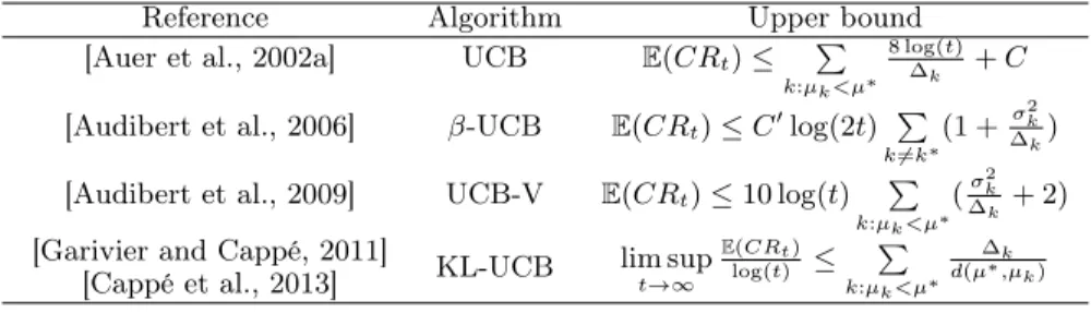
2.3 Multi-Armed Bandit

The multi-armed bandit problem [Auer et al., 2002a, Katehakis and Veinott Jr, 1987] is an important model of exploration/exploitation trade-offs, aimed at optimizing the expected payoff. It is related to portfolio methods, as they are natural candidates for select-ing the best algorithm in a family of solvers dependselect-ing on their payoffs. The concepts defined here will be used throughout the present document: adversarial bandit algorithms for computing Nash equilibria, bandit algorithms for portfolio methods in noisy optimization; and in Monte Carlo Tree Search, used in some of our experiments.