Deceleration of antiprotons from CERN’s ELENA synchrotron and transport of antimatter beams through the GBAR experiment

(1)

HAL Id: tel-02526874

https://tel.archives-ouvertes.fr/tel-02526874

Submitted on 31 Mar 2020

HAL is a multi-disciplinary open access

archive for the deposit and dissemination of

sci-entific research documents, whether they are

pub-lished or not. The documents may come from

teaching and research institutions in France or

abroad, or from public or private research centers.

L’archive ouverte pluridisciplinaire HAL, est

destinée au dépôt et à la diffusion de documents

scientifiques de niveau recherche, publiés ou non,

émanant des établissements d’enseignement et de

recherche français ou étrangers, des laboratoires

publics ou privés.

synchrotron and transport of antimatter beams through

the GBAR experiment

Audric Husson

To cite this version:

Audric Husson. Deceleration of antiprotons from CERN’s ELENA synchrotron and transport of

antimatter beams through the GBAR experiment. General Relativity and Quantum Cosmology

[gr-qc]. Universite Paris Saclay, 2018. English. �tel-02526874�

(2)

NNT

:2018SA

CLS255

Deceleration of antiprotons from CERN’s

ELENA synchrotron and transport of

antimatter beams through the GBAR

experiment

Thèse de doctorat de l’Université Paris-Saclay préparée à Université Paris-Sud, au CSNSM Ecole doctorale n◦_{576 Particules, Hadrons, Energie, Noyau, Instrumentation,}

Imagerie, Cosmos et Simulation (PHENIICS)

Spécialité de doctorat : Physique des Accélérateurs

Thèse présentée et soutenue à Orsay, le 17/12/2018, par

A

UDRIC

HUSSON

Composition du Jury : Mme Amel KORICHI

Directrice de recherche, CNRS (CSNSM) Pr´esidente

M. Patrick NEDELEC

Professeur, Universit´e Lyon 1 (IPNL) Rapporteur

M. Christian CARLI

Docteur, CERN (BE/ABP) Rapporteur

M. David LUNNEY

(3)

(4)

(5)

(6)

List of Figures

1.1 Cloud Chamber photograph by C.D. Anderson - 1933 . . . 15

1.2 Energy-loss in the ALICE-TPC for P b − P b collission at 2.76 T eV - 2016 . . 16

1.3 Schematic diagram of the Witteborn-Fairbank apparatus - 1968 . . . 22

1.4 Schematic diagram of the PS200 experiment - 1987 . . . 23

1.5 Antiproton Decelerator hall layout - 2014 . . . 25

2.1 Total cross section for the double charge exchange reaction with different laser excitations of the positronium - 2013 . . . 28

2.2 Schematic illustration of the GBAR experiment. . . 29

2.3 Layout of the GBAR experiment in the CERN AD hall. . . 29

2.4 GBAR LINAC and positron source - 2018 . . . 30

2.5 Principle scheme of the buffer gas trap - 2017 . . . 31

2.6 Picture of the positron accumulation trap. . . 31

2.7 Sketch of the ¯p − P s interaction region. . . 32

2.8 oPs formation principle - 2010 . . . 32

2.9 Be+ _{ion Coulomb crystal - 2018 . . . .} ₃₃

2.10 Pictures of the GBAR precision trap - 2014 . . . 34

2.11 Sketch of the GBAR free-fall chamber - 2017 . . . 35

2.12 Principle scheme of the GBAR decelerator. . . 35

2.13 Sketch of the switchyard and the pulsed drift tube assembly from the TRIGA-TRAP apparatus - 2012 . . . 36

3.1 Shape of the potential applied on a decelerating tube without switching it to ground and antiproton simulated trajectories - 2018 . . . 41

3.2 Shape of the axial potential V (z, 0), its first and second derivatives computed with the SIMION software. . . 45

3.3 Illustration of the chromatic aberration effects in the case of an Einzel lens -2018 . . . 46

3.4 Definition of the δd distance and projection of the potential at the entrance of the drift tube - 2018 . . . 47

3.5 Axial potential variation along the PDT wrt the distance δd - 2018 . . . 48

3.6 Radial potential variation in the PDT - 2018 . . . 49

3.7 Schematic of the pre-prototype shape of the GBAR decelerator - 2018 . . . . 50

3.8 Definition of the principal planes and focal points in an electrostatic gap - 2018 51 3.9 Schematic of the principal planes and focal points for the GBAR drift tube for a 100 keV antiproton beam - 2018 . . . 51

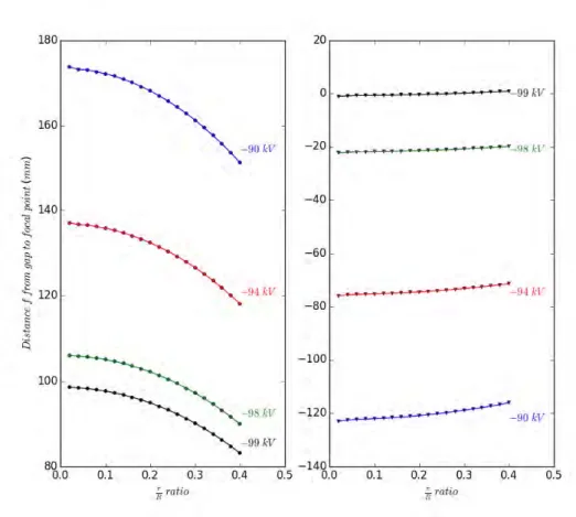
3.10 Comparison of simulated telescopic systems for a 1 keV deceleration - 2018 . 52 3.11 Position of the focal point object (left) and image (right) with respect to the radial position of the incoming particles in the PDT - 2018 . . . 53

3.12 Phase space ellipse representation of the beam on one axis - 2014 . . . 54

3.13 Simulation of the influence of the nearest electrodes on the potential along the optical axis - 2018 . . . 56

4.1 Schematic diagram of a typical evolutionary algorithm. . . 59 7

(9)

4.2 Examples of crossover processes - 1989 . . . 63

4.3 Evolution of the phenotype ratios in a bird population over 400 generations -2018 . . . 66

4.4 Schematic of the search algorithm. . . 67

4.5 Phase space distribution of the simulated beam. . . 70

4.6 Schematic of the prototype design of the decelerator. . . 74

4.7 Comparison of the "4m Minimize Alpha" beam through the preliminary design - 2018 . . . 75

4.8 Systematic calculation method for the 1R1R electrostatic configuration through the prototype design of the decelerator - 2017 . . . 76

4.9 Comparison of the refocusing impact downstream the PDT - 2018 . . . 79

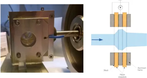
5.1 Picture and schematic of the prototype off-line decelerator test bench - 2016 . 81 5.2 Triplet of pre-decelerating electrodes mounted on the aluminum frame with Macor rods. . . 82

5.3 Picture and schematic of the energy analyzer - 2015/2018 . . . 82

5.4 Schematic of the Orsay Penning-type discharge source - 2016 . . . 83

5.5 Picture of a collimator and of the Orsay source - 2016 . . . 84

5.6 Picture and simulation of the Orsay Wien filter - 2016 . . . 86

5.7 Wien filter spectrum of the Penning-type source. . . 86

5.8 TOF spectrum signal and simulation for the Orsay ion source - 2016 . . . 87

5.9 Picture of the BEHLKE HTS 1501-20-LC2 single pole, single throw (very) high voltage switch - 2015 . . . 88

5.10 Picture of the BEHLKE HTS 1401-20-GSM single pole, double throw (very) high voltage switch. . . 89

5.11 PDT potential measured through a 1 : 100₀₀₀_{divider probe during a complete} 1sswitching cycle on the decelerator . . . 90

5.12 Schematic of the pulsed high voltage circuit when working with (a) - the SPST switch or (b) - the SPDT switch . . . 91

5.13 Picture of the high voltage assembly in the SPST configuration . . . 93

5.14 Picture of the pulsed high voltage circuit embedded in its dielectric shield inside the copper Faraday cage . . . 94

5.15 Photograph of a high voltage feedthrough mounted on the decelerator chamber 94 5.16 MCP signal while decelerating from ∼ 50 keV to 1 keV . . . 95

5.17 Time of flight spectra from the discharge source successively non-decelerated and decelerated . . . 96

5.18 Energy spectra after the deceleration . . . 97

5.19 Photograph an Einzel lens doublet as used for the refocusing system. . . 98

5.20 Schematic of the refocusing test bench . . . 98

5.21 Photograph of the hat-shaped mask mounted in front of the Faraday Cup detector. . . 99

5.22 Beam current as measured on the hat-shaped mask and in the Faraday Cup for a 2 − keV proton beam . . . 99

5.23 Misalignment illustration of the beam current as measured on the hat-shaped mask and in the Faraday Cup for a 2 − keV proton beam . . . 100

5.24 Photograph of the on-line decelerator in the AD Hall . . . 101

5.25 Picture of a flat port on the side of the in-line decelerator chamber and picture of the inside of the in-line decelerator chamber . . . 102

5.26 Schematic of the on-line decelerator in the new chambers with the electrode positions and dimensions . . . 103

5.27 Schematic and picture of the improved energy analyzer. . . 104

5.28 Schematic of the MCP-EA test bench. . . 105

5.29 Test of the MCP-EA with different beam energies . . . 106

5.30 Test of the MCP-EA with different beam energies (bis) . . . 107

(10)

List of Figures 9 5.32 The ELENA extraction line (LNE50 ) that delivers beam to GBAR . . . 109 5.33 The GBAR injection line that receives beam (coming from the left) from the

ELENA LNE50 extraction line . . . 109 5.34 Schematic diagram of the antiproton line, showing the positions of the optical

elements and different detectors . . . 110 5.35 Photograph of the antiproton beam line with the new decelerator chambers . 110 5.36 MCP/PS image of the antiproton beam and oscilloscope traces . . . 111 5.37 Schematic of the reaction chamber . . . 112 5.38 MCP/PS image of the antiproton beam and oscilloscope traces (bis) . . . 113 6.1 Geometry of the T2P (top) and CPB (bottom) designs as modeled in SIMION.

The blue lines correspond to antiprotons flying from left to right through the bender. The red rectangle displays the PPs converter position. The CCPB de-sign is not represented but is equivalent to the CPB dede-sign (top) with grounded

gate at the entrance and exit of the beam. Note the particular orientation where the X-axis corresponds to the beam propagation direction. . . 116 6.2 Beam Profile comparison between the beam at the entrance and exit of the

T2P design switchyard . . . 118 6.3 Transverse (Y-)speed distribution comparison at the entrance and exit of the

T2P design . . . 118 6.4 Beam Profile comparison between the beam at the entrance and exit of the

CPB design . . . 119 6.5 CPB and CCPB phase space diagrams comparison. . . 119 6.6 Drawing of the switchyard vacuum chamber DN300CF standard with ±30◦

port plus 0◦_{other ports. . . 120}

6.7 Picture of the switchyard optics mounted in their vacuum chamber . . . 121 6.8 TOF spectrum and TOF versus energy diagram of a time-focused antiproton

beam 2.4 m downstream the decelerator . . . 123 6.9 Total cross sections for positronium atoms, in the specified initial state nl,

scattering on (anti)protons to form (anti)hydrogen calculated by using the CCC methods . . . 123 6.10 GBAR antiproton trap electrodes. . . 124 6.11 Fraction of trapped antiprotons according to SIMION simulations using two

lenses . . . 125 6.12 Fraction of trapped antiproton according to SIMION simulations using a single

lens downstream of the decelerator . . . 125 6.13 Schematic of the TES35 proton source integrated in the GBAR experiment.

Data from the Polygon Physics company. . . 127 6.14 Molflow simulation of the GBAR proton source line . . . 128 6.15 Photograph of the separation of the different species extracted from the TES35

source by a magnet . . . 129 6.16 SIMION simulation of the GBAR proton line optics . . . 129 6.17 Profiles of the proton beam 1 m downstream the quadruple bender in the

decelerator chamber . . . 130 A.1 Appendix a - The unitary potential electrode divided in dζ−large slices. . . . 148 A.2 Appendix A - Infinitely long conducting cylinders with finite separation S;

potential along cylinder surface. . . 149 A.3 Appendix A - Example of potentials along a concentric multi-electrode system. 150 B.1 Appendix B - Differential pumping assembly for the GBAR proton source. . . 152 B.2 Appendix B - Differential pumping diagram . . . 153 C.1 Appendix C - Design of the two-stage deceleration apparatus . . . 155 C.2 Appendix C - Beam characteristics through the two-stage deceleration apparatus156

(11)

D.1 Appendix D - New GBAR decelerator - Chamber 1. . . 158

D.2 Appendix D - New GBAR decelerator - Chamber 2. . . 159

D.3 Appendix D - New GBAR decelerator - Chamber Pulsed Drift Tube. . . 160

D.4 Appendix D - New GBAR decelerator - Chamber Einzel lens. . . 161

D.5 Appendix D - High voltage brass ball connector. . . 163

D.6 Appendix D - High voltage feedthrough connector. . . 164

D.7 Appendix D - High voltage resistor-cable connector. . . 165

D.8 Appendix D - High voltage Teflon support - Part I. . . 166

D.9 Appendix D - High voltage Teflon support - Part II. . . 167

(12)

List of Tables

1.1 Progress in the evaluation of the Eötvös parameter ηE . . . 20

4.1 Initial bird population . . . 65

4.2 Preliminary Twiss parameters of the beam ejected from ELENA . . . 71

4.3 Solutions proposed by the execution of the Genetic Algorithm . . . 72

4.4 Beam parameters in the drift tube for the 1P 1R electrostatic configuration. . 73

4.5 Beam parameters in the drift tube for the 1R1R electrostatic configuration. . 74

5.1 Ionization processes in hydrogen gas with respect to the electron impact energy - 1990 . . . 84

6.1 Beam parameters for the different designs proposed for the switchyard . . . . 117

6.2 Results for the switchyard with a better defined initial beam . . . 120

6.3 Proportion of the charged species extracted from the TES35 source . . . 128

B.1 Appendix B - Evaluation of the conductance, gas flow and pressure through the differential pumping line. . . 153

(13)

(14)

Chapter 1

Introduction

Einstein’s theory of General Relativity (GR) is arguably one of the greatest scientific achievements ever. This elegant theory still awaits expression in the language of quantum physics - somehow now achieved for all of the other fundamental interactions of nature. The cornerstone of GR is the Weak Equivalence Principle (WEP) which expresses the equivalence of inertial and gravitational mass.

Numerous theoretical and experimental investigations proved that the gravitational mass and the inertial mass of ordinary matter are equivalent to one part per 1012_.

Point-ing out the lack of evidence considerPoint-ing the gravitational behavior of antimatter systems, theorists have built new models that in some cases violate CPT or Lorentz invariance as an explanation for baryogenesis or cosmological problems.

With advances in antimatter synthesis, tests of the WEP with antimatter are now achievable. Considering the weakness of gravity compared to any residual electrical or magnetic force, direct free-fall experiments with charged antimatter appear unrealistic. Antihydrogen is the best candidate because of its electrical neutrality and its lifetime com-pared to other neutral anti-systems like positronium atoms (P s). But this apparent ad-vantage implies the use of complicated systems to trap neutral atoms. Such trapping tech-niques have already been performed by antimatter experiments such as AT RAP [1, 2, 3], ASACU SA [4, 5, 6] and ALP HA [7, 8, 9].

Even if these collaborations have already managed to synthesize antihydrogen atoms, the measurements of F = Mg/MI, defined as the ratio of the gravitational mass Mg to

the inertial mass MI of antihydrogen, remains quite difficult.

In this chapter, a retrospective of the discoveries around antimatter is made as well as a summary of the great theories in particle physics and relativity. Finally, a panorama of attempts to measure the gravitational behavior of antimatter is presented.

(15)

1.1 Antimatter discovery

1.1.1 Dirac equation and the negative solution problem

In 1928, Paul A. M. Dirac by means of an innovative theoretical concept, obtained a relativistic theory of the electron. While major physicists of the time, like Oskar Klein or Walter Gordon, were already working on a relativistic equation, referred to as the Klein-Gordon equation, Dirac solved the problem of negative probability density func-tions by introducing a solution not based on a one dimensional wave function but on a four-dimensional wave function, called a spinor. Equivalent to four parallel Schrödinger equations with mixing terms1_{, the equation can be formulated as:}

i h 2π ∂Ψ ∂t = −i h 2π~α.~∇Ψ + βmc 2 Ψ (1.1)

where Ψ is a four-dimensional wave function; m, the mass of the particle, c the speed of light; h, Planck’s constant and ~α,β are the 4x4 matrices acting on spinors, also known as Dirac’s matrices.

This equation addresses the problem of the negative probability density while rigor-ously describing the spin, the magnetic moment and the spin-orbit interaction of the elec-tron [10, 11]. However this equation raises a new problem; when a simple two-dimensional wave function may describe the electron spin states what happens to the other two di-mensions ? Moreover, if the positive solutions of this equation describe the electron, what about the negative solutions ?

"The relativity quantum theory of an electron moving in a given electro-magnetic field, although successful in predicting the spin properties of the electron, yet involves one serious difficulty [...] connected with the fact that the wave equation [...] has, in addition to the wanted solution for which the kinetic energy of the electron is positive, an equal number of unwanted solu-tions with negative kinetic energy for the electron, which appear to have no physical meaning."

Paul Dirac, 1930 In 1929, Hermann Weyl suggested that the negative energy solutions (and positive charge) stand for protons [12]. Dirac demonstrated that such a hypothesis leads to a violation of the electric charge conservation and postulated that vacuum is made of an infinite number of negative energy levels (later referred as the Dirac sea). Following this idea, if enough energy is transferred to a negative energy electron, it becomes a real elec-tron (with positive energy) leaving a hole in the ’sea’.

"A hole, if there were one, would be a new kind of particle, unknown to experimental physics, having the same mass and opposite charge of the electron."

Paul Dirac, 1931 [13] In 1931, Dirac put forward the controversial2_{, but equally ingenious hypothesis that}

holes could be interpreted as new particles.

1_{In the low velocity approximation, one can find the Schrödinger equation : i}h

2π ∂Ψ ∂t = − 1 2m( h 2π) 2_∇2_Ψ

(16)

1.1. ANTIMATTER DISCOVERY 15

1.1.2 From theory to experiment : antimatter under the spotlight

In 1932, Carl Anderson discovered that, high energy photons from cosmic rays interact-ing with a lead screen, produce electrons as well as particles with almost the same mass but with opposite charge [15] as shown in Figure-1.1. Furthermore, these new particles can be converted back into two photons. The discovery was confirmed at the Cavendish Laboratory (Cambridge) by Patrick Blackett and Giuseppe Occhialini in 1933 [16].

The same year C.D. Anderson named this new particle, today interpreted as an anti-electron, positron [17]. Subsequently, as a confirmation, Irène and Frédéric Joliot-Curie identified positrons in the β+ _{decay process of a phosphorus isotope [18] following:}

30_{P →}30_{Si + e}+_{+ ν}

Nevertheless, the Dirac equation in (1.1) is not only valid for electrons but for any spin-½ particles. Indeed, following this idea, the proton and the newly discovered neutron [19] should also present a corresponding anti-partner with the same mass but with opposite spin.

Figure 1.1 Cloud chamber photograph by C.D. Anderson [17]. A 63 MeV positron passed through a 6 mm lead plate and emerged at 23 MeV . The length of this path is at least 10 times greater than the possible trajectory of a proton with the same curvature.

Antiproton Discovery In 1955, after some minor unconfirmed cosmic-rays events [20, 21, 22], Emilio Segrè and Owen Chamberlain discovered the proton antimatter counter-part, named antiproton (¯p or pbar) [23]. They used the novel proton accelerator, called the Bevatron, at the Lawrence Berkeley National Laboratory designed to achieve a 6.5 MeV energy, which corresponds to the threshold that produces proton-antiproton pairs im-pinging an initial proton beam on a copper target. The detection of the antiprotons was performed via a momentum and time-of-flight identification, since the main contaminant particles were negative mesons produced in the reaction with a higher momentum.

(17)

Additional antimatter discoveries One year later, in 1956, following the same TOF discrimination principle in the same laboratory, the team of Oreste Piccioni and Bruce Cork discovered the neutron counterpart, the antineutron (¯n) [24].

After single antiparticles, the production of antimatter turned to antinuclei, such as: anti-deuterons ( ¯d) at Brookhaven first [25] and few months later in Europe at CERN in 1965 [26], antihelium-3 nuclei (3_{He) in 1971 [27] and antitritons (}_¯ 3_H_¯(+)_{) in 1974 [28].}

In 1995, a new step was taken by the LEAR (Low Energy Antiproton Ring) experi-ment at CERN. Colliding an antiproton beam circulating in a ring with a Xenon gas jet, the first (and simplest) atomic structures made of antimatter, antihydrogen atoms ( ¯H), were synthesized. 11 events were recorded (with an hypothetical background of 2 ± 1 events) [29].

Furthermore, in 2010, the STAR experiment at RHIC, Brookhaven National Labora-tory, announced the discovery of the first anti-hypernucleus, the antihypertriton (3

¯

ΛH¯) [30].

All these discoveries have been recently confirmed at high energy by the ALICE experi-ment, CERN-LHC [31, 32] as summarized in Figure-1.2. They also reported the discovery of antihelium-4 nuclei (4_He)._¯

Figure 1.2 Energy-loss as measured in the Time Projection Chamber (TPC) of the ALICE experiment. The black lines correspond to the expected energy loss for different particles-antiparticles and nuclei-antinuclei. Data taken in lead–lead collisions at 2.76 T eV [33].

(18)

1.2. (ANTI-)ATOMS IN AN (ANTI-)UNIVERSE 17

1.2 (anti-)atoms in an (anti-)Universe

The relativistic interpretation of the quantum theory gave birth to a new family of par-ticles. As proof of his genius, Dirac is also at the origin of a theory today considered as the very first step of the quantum field theory[34]3_{. This latter is undeniably one of the}

greatest achievements in modern physics describing three of the four known interactions (electromagnetism, weak and strong interactions).

The quantum field theory formalism implies that physical laws stay unchanged under the successive combined transformations:

• C-symmetry: charge conjugation, switching all particle properties with those of their corresponding antipartners.

• P-symmetry: parity transformation, opposing the spatial coordinates • T-symmetry: time reversal

If there is no more doubt on the C-symmetry and P-symmetry violation in the weak sector [35, 36] and moreover on the combination of both CP-symmetry [37, 38, 39, 40], there is no hint yet of the violation of the CPT-symmetry4_.

Today, the invariance of the physical laws under the above CPT combination is widely recognized as an indisputable truth. The CPT-invariance implies that the inertial mass, charge magnitude, mean life and magnetic moment are identical for any particle and its corresponding antiparticle. One of the main goals of the current low-energy antimatter experiments is to confirm this statement. A non-exhaustive list of the last results can be found in Refs.-[7, 41, 42, 43, 44, 45, 46, 47, 48].

According to the invariance of the physics laws with respect to the CPT-symmetry, a major question remains partly unanswered : why are we made of matter and not anti-matter ?

Astronomical observations show that in the observable Universe, antimatter particles are sporadically present. It means that no matter and antimatter macroscopic structures coexist in our close neighborhood. Indeed, such coexistence would lead to the emission of radiation coming from a large number of annihilations at the frontier between matter and antimatter.

The Standard Model of particle physics associated with the ΛCDM-model (or Stan-dard Cosmological Model) explains at best the composition of our visible Universe. Shortly after the Big Bang, matter and antimatter are produced with almost5 _{the same}

abun-dance. The coexistence of particles and antiparticles lead to annihilation processes pro-ducing the current observed photons. At the end of this phase, all particle-antiparticle couples disappeared. The exceeding particles remain forming the Universe as we know it. Hints of this original event are still detectable by estimating the baryon-to-photon ratio in our visible Universe, also referred as baryon abundance η = nb/nγ, with nb the

number density of baryon and nγ the number density of relic blackbody photons.

Ac-cording to [49], recent cosmological evaluations6_{: 5.8×10}−10_{≤ η ≤ 6.6 × 10}−10_{. It means}

3_{The new quantum electrodynamic (QED) theory is the fruitful work of successive ingenius physicists}

whose apotheosis is reached in 1949 with the work of Julian Schwinger, Sin-Itiro Tomonaga and Richard Feynman.

4_{Considering the CPT symmetry, one should note that a violation of the CP-symmetry induces a}

violation of the T symmetry.

5_{The quasi-equality is here of crucial importance.}

6_{The number density of relic blackbody photons is fixed by the Cosmic Microwave Background}

tem-perature T = 2.7255(6) K to nγ = 410.7(3) cm−3. The baryon density nbin the standard Big Bang

(19)

that almost one particle over 109 _{survived to the primordial annihilation.}

Following this estimation, particle physicists and cosmologists have tried to explain this asymmetry. In 1966, Andrei Sakharov proposed an explanation [50] based on three conditions (referred as the Sakharov conditions):

1. The C- and CP-symmetry violation allows matter and antimatter to interact differ-ently.

2. The violation of the baryon conservation law that explains the excess of baryons over antibaryons.

3. Interactions must be out of thermal equilibrium.

As described in the previous subsections, several experiments already established the violation of the C- and CP-symmetry. Moreover, the expansion phase during the early age of the Universe (when the annihilation process occurred) can be seen as an out-of-equilibrium system where particles and antiparticles do not achieve a thermal out-of-equilibrium. Unfortunately, no evidence of a broken baryon conservation law has yet been brought to light and still need to be found7_.

In parallel with the Sakharov conditions, another exotic hypothesis suggests the co-existence of matter and antimatter in equal quantities in the Universe. The absence of irradiating interface could be explained by an asymmetry in the gravitational behavior of antimatter with respect to matter [51, 52]. This Kant-like perspective of an ’antimat-ter island Universe’ is unlikely at our scale and is not supported by recent cosmological observations on the Cosmic Microwave Background.

1.3 "Defying gravity"

Before drawing hasty conclusions about the disappearance of antimatter beyond the vis-ible horizon, one should understand how gravity applies and what could differ from the behavior of matter.

1.3.1 The (not so) Weak Equivalence Principle

When physicists have to deal with macroscopic low energy experiments, they inevitably deal with Einstein’s theory of General Relativity. This theory relies on postulates con-fronted by nearly one century of experimental tests without fault, among them the Equiv-alence Principle.

In its weak form or Weak Equivalence Principle (WEP), it asserts that in a grav-itational field the acceleration of a "test particle" is independent of its mass and its composition but only depends on its initial position and velocity [53]. This principle is also called the Universality of Free-Fall (UFF ). In the framework where the gravitational acceleration is indistinguishable from a mechanical acceleration, it is equivalent to say that gravitational mass is identical to inertial mass. When associated with the Local Lorentz Invariance (LLI ) and the Local Position Invariance (LPI ), this principle is known as the Einstein Equivalence Principle (EEP) and is at the foundation of the Einstein’s Special and General Relativity theory.

and the Newtonian constant of gravitation GN. It is now fixed to nb = 2.503 × 10−7 cm−3. Larger

references in [49].

7_{The baryon (and/or lepton) number violation can be accommodated in the Standard Model of}

(20)

1.3. "DEFYING GRAVITY" 19 This Equivalence Principle is qualified as weak as opposed to the Strong Equivalence Principle whose demonstration is based on a pure geometrical approach of space-time and requires a more detailed but also constraining definition. This latter aims to generalize the WEP to any place in the Universe even in regions where the gravitational field suf-fers from important distortions8_{. The violation of such SEP would rest on the variation}

of fundamental constants, like the (Newton’s) Gravitational Constant over time like for instance at the early age of the Universe or close to massive cosmological structures.

1.3.2 From theory to experiment

The EP has been the cornerstone of all gravity theories since Galileo’s work 400 years ago. By investigating the motion of objects on inclined planes and pendulums9_{, he}

un-derstood that objects of different mass and composition accelerate similarly in the same gravitational field and formulated the first empirical law of free-falling bodies.

The first mathematical description of gravity was published by Sir Isaac Newton in 1687 in the famous Pincipia. By applying his second law, Newton considered the funda-mental difference between the inertial and gravitational mass [54]. Let’s consider Newton’s law of motion for a free-falling body:

~

F = minertial~a ;with ~F = mgravitational~g then, ~a =

mgravitational minertial ~g

After testing his theory via the use of pendulums with different mass and composi-tion, he found no deviation from mgravitational/minertial = 1with 10−3 accuracy. Using

pendulums as well, Bessel improved this limit to 1 part per 105 _{in 1832. In 1889, Loránd}

Eötvös used an innovative system composed of a torsion balance. He demonstrated ex-perimentally the equality with an accuracy of 1 part per 109_{[55, 56].}

More than a century later, the mass identity is still of interest for various theoretical and experimental investigations. Most of the experiments challenging the EP are based on the comparison of the acceleration of test bodies made of different compositions. Paying tribute to the Baron von Eötvös, a new dimensionless parameter has been defined to quantify the equivalence between the inertial and gravitational mass. For two test bodies defined as A and B, the Eötvös parameter η is:

η(A, B) = ∆a aS = 2.0 (aA− aB) (aA+ aB) = 2.0 ( mg mi)A− ( mg mi)B (mg mi)A+ ( mg mi)B (1.2) with mg and mi, respectively the gravitational and inertial mass, ∆a the hypothetical

difference in acceleration and aS the average acceleration.

In recent decades, the η parameter has continued to be lowered (cf Table-1.1). Its measurement and the test of the UFF is still necessary to test Einstein’s theories at the highest level.

An important element one should notice, is the apparent simplicity of the experiments in Table-1.1. The use of a torsion balance or a test mas in a satellite orbiting around the Earth offer the possibility to confirm the WEP with a maximum accuracy of 10−15_.

Is such a precision achievable for testing antimatter ? Could a deviation explain its disappearance ?

8_{The EEP require to work in local constant gravitational potential and then do not take into account}

for instance tidal effects induced by the rotation of the Earth or the revolution of the Moon.

(21)

Year Authors Limit on Method & η = |∆a/a| Reference parameter 1590 Galileo 2.10−2 Pendulum 1687 Newton [54] 10−3 Pendulum 1832 Bessel 2.10−5 Pendulum 1908 (1922) Eötvös [55, 56] 2.10−9 Torsion Balance 1918 Zeeman 3.10−8 Torsion Balance 1935 Renner 2.10−9 Torsion Balance 1964 Dicke, Roll, Krotkov [57] 3.10−11 _{Torsion Balance}

1972 Braginsky, Panov 10−12 _{Torsion Balance}

1976 Shapiro, et al. [58] 10−12 _{Lunar Laser Ranging}

1987 Niebauer, et al. [59] 10−10 _{Drop Tower}

1989 Stubbs, et al. [60] 10−11 _{Torsion Balance}

1990 Adelberger, Eric G.; et al. [61] 10−12 _{Torsion Balance}

1999 Baeßler, et al. [62] 5.10−14 _{Torsion Balance}

2003 V. Nevizhevsky, et al. [63] 0.2 % Neutron free-fall 2016 MICROSCOPE [64] 10−15 _{Earth Orbit}

Table 1.1 Progress in the evaluation of the Eötvös parameter ηE

1.4 What about antigravity ?

A gravitational asymmetry seems impossible holding as exact the GR theory with the EEP principle. But regarding the expansion mechanism and the composition of our Universe, theorists have developed new models including matter-antimatter gravitational asymmetry. For instance, Nieto and Goldman supported this point of view (cf. Ref.[65], Section 8) conjecturing a possible "fifth force" among the current gauge forces of the Standard Model (SM ) without any contradiction with GR.

"... the more precisely anomalous gravitational effects are ruled out in earth-based matter-matter experiments, the more unrestricted is the possi-bility that there can be a significant anomalous gravitational acceleration of antimatter"

Nieto & Goldman, 1991, [65] There is also no obvious evidence concerning CPT-symmetry. While many experi-ments rigorously proved the correctness of CPT for asymptotically flat-space relativistic local field theories, some Standard-Model Extensions (SME) assume a possible violation. Indeed, CPT-symmetry does not impose constraints on how antimatter interacts with a gravitational field induced by a matter structure. If one considers a simple gravitational experiment of a falling apple on Earth, the strict application of the CPT-symmetry means therefore to drop an "anti-apple" on an "anti-Earth".

1.4.1 Indirect estimation

A consequence of the WEP is a gravitational redshift [66]. For oscillatory systems, this latter is characterized by a shift in the observed frequencies compared to expectations with respect to the position of the studied system in the gravitational field.

(22)

1.4. WHAT ABOUT ANTIGRAVITY ? 21 We can here define a new parameter, the matter-antimatter gravitational coupling α as:

¯

g = αg (1.3)

with g and ¯g, the gravitational accelerations of matter and antimatter respectively. One can easily derive from (1.3) in the framework of a free-fall that :

α = MA¯

MA

⇐⇒ |1 − α| = ∆MA¯−A MA¯

(1.4) where A represents a test mass and ¯Aits antimatter counterpart, M the gravitational mass of A/ ¯A.

Attempts to establish a limit on the WEP with antimatter have already been per-formed. By measuring, the K0_{− ¯}_K0_{oscillation rate [37, 67, 68] or the proton/antiproton}

cyclotron frequency [69, 70, 71], one can extract an indirect limit on the gravitational asymmetry between matter and antimatter.

∆Mg.φg∝ ∆ω with φ =

GM

Rc2 (1.5)

∆Mg is the equivalent mass difference between matter and antimatter, GM the standard

gravitational parameter, R the orbital radius, c the speed of light and ∆ω the gravitational redshift10

The limits found are :

|1 − α| ≤ 2.0 × 10−13 from neutral kaon mixing [68]

|α − 1| < 5 × 10−4 from cyclotron frequency measurement [71]

If such results seems indisputable, a controversial argument emerges from their anal-ysis. Indeed, the above values are established using the supergalactic cluster (the "great attractor") as the dominated excess mass. But the definition of the excess mass ref-erence (the Earth, the Sun, the galactic nucleus or the supergalactic cluster) leads to different values of |1 − α| with several orders of magnitude difference. As emphasized in reference-[72, 65] and in Ref.[66]-Section 5.4, the evaluation of the |1 − α| = ∆M/MA

value is still subject to a debatable definition and does not constitute an irrefutable proof.

1.4.2 Astronomical observations

On 23rd_{February 1987}11_{, a type-II supernova exploding in the Large Magellanic Cloud [73]}

offered the opportunity to highlight a possible gravitational asymmetry. Three hours be-fore the supernova appeared in the sky, a neutrino burst was detected in two different neutrino experiments: 11 events reported at Kamiokande II (Japan) [74, 75] and 8 events in IMB (USA) [76].

According to Ref.[77] and [78], these 19 events revealed statistically no difference in the arrival time of neutrinos, antineutrinos and photons. Demonstrating that (anti-)neutrinos and photons follow the same trajectories in the gravitational field of the galaxy, Krauss and Tremaine [78] estimated the WEP to be true with an accuracy of at least 0.5%. Considering at least one νeevent, the autors of Ref.[79] derived the WEP to be validated

to an accuracy of one part per 106_.

10_{In the case of Ref.[71], the redshift is defined as a difference in the measured antiproton cyclotron}

frequency compared to proton one. In the case of the K0− ¯K0_{oscillation, it corresponds to the difference}

between their de Broglie frequencies define according to Ref.[68].

(23)

But again, the hypothesis used for the gravitational potential and the excess mass reference12_{is questionable. Furthermore, the difficulty to differentiate between neutrinos}

and antineutrinos and to clearly establish the flavor of the detected events raised the problem of their origin.

Despite other theoretical attempts to glimpse an asymmetry in the gravitational cou-pling for instance in (anti-)neutrino mixing between flavor eigenstates [80] or even in the solar neutrino "deficit" [81], no evidence has supported these theories so far.

1.4.3 Direct attempts

Seeing the limits of the indirect measurements, only direct tests seem to offer a level of confidence high enough to test the WEP. Considering the difficulty to synthesize antimat-ter and the incompatibility of mixing matantimat-ter and antimatantimat-ter, torsion-balance or pendulum experiments are obviously unfeasible with antimatter.

Figure 1.3 Schematic dia-gram of the helium-immersed portion of the Witteborn-Fairbank apparatus.

However, the neutron free-fall experiment13

per-formed in 2003 [63] presents an interesting perspec-tive for direct observation. Valery Nesvizhevsky and his team used Ultra-Cold Neutrons (UCN ) to realize a single particle free-fall experiment. Such a free-fall test with antineutrons is unrealistic because the cool-ing and guidcool-ing processes that involve scattercool-ing and bouncing off of matter [82]. Nevertheless, improve-ments in antimatter trapping and cooling techniques for non neutral antimatter systems offer the possibility to reach energies low enough to observe gravitational ef-fects.

In 1968, Witteborn and Fairbank proposed a direct measurement using cold electrons and positrons [83, 84, 85]. As shown in Figure-1.3, this experiment is based on the analysis of the time-of-flight distribution of electrons (resp.: positrons) falling freely within a shielded vacuum chamber. A cryogenic source at the bottom of the cavity emits cold electrons upwards in a fountain-like mode. A Multi-Channel Plate faces the source on the top of the cavity. The electrons are constrained to move along the axis of the vacuum cavity by a magnetic field of a coaxial superconducting solenoid. Residual fields mainly result from induced image and are reduced by surrounding the free-fall region with copper drift tubes (cf Figure-1.3).The charged particles experience an effective gravitational ac-celeration:

gef f = g(1 − Qme/eM )

where Q and M are the charge and mass of the particle.

12_{The references [77] and [78] used the galaxy and the galactic nucleus as excess mass reference.}

(24)

1.4. WHAT ABOUT ANTIGRAVITY ? 23 If all the residual forces are suppressed, the distribution of the electrons or positrons time of flight should display a cut off at tcutof f = p2mh/mg = p2L/g with the drift

tube length L. F.C. Witteborn and W.M. Fairbank found that for the electron, gef f was

less than 0.09g. A simple calculation gives an estimation of gef f = 2gin the positron case.

Considering the gravitational potential gradient of an electron or a positron at the Earth’s surface equivalent to mg = 5.6 10−11_eV.m−1_{, all vertical electric and magnetic}

gradients must be reduced below the 10−11 _{eV /m} _scale14_{. But even working in an}

in-sulating box with at least one trapped charge inside would lead to a force greater than mg. Systematic errors overwhelm all measurements. After several attempts and thorough research of noise sources, the result of gef f = 0.02g for electrons has not convinced the

antimatter community [86] and no attempt has been made for positrons.

Following a similar method but with antiprotons, the PS200 experiment [87] (Fig.-1.4) accepted by CERN based on the capture and cooling of antiprotons into a Penning trap to make the same free-fall test as in the Witteborn-Fairbank’s experiment. This experiment was installed at the LEAR facility, unfortunately this antiproton investigation stopped without any evidence. It seems realistic to suppose that such an experiment would suffer from the same systematics problems.

Figure 1.4 Schematic diagram of the apparatus for the proposed experiment PS200, based on Ref.-[88]

The previous attempts to test the WEP with single free-falling charged particles ex-hibit the most important problem in such gravity experiment: the lightness of particles. For instance, the ratio of the electrostatic and gravitational forces between two protons at 1m distance is tremendous:

(25)

Electrostatic Force : FE = kCq1.q2_d2 → F = 2.3 × 10−28 N Gravitational Force : FG = Gm1_d.m2 2 → F = 1.87 × 10−64 N ) FE FG ≈ 1036

Even if the associated technology has been improved, reaching a level of residual field lower than 10 fV/m = 10−11 _{V /m} _{appears quite challenging. The obvious conclusion}

is to perform such a free-fall test with neutral antimatter systems. Such experiments are now being pursued using laser cooling and velocity techniques to measure the time of flight or to measure the position in a magnetic antihydrogen trap. These experiments will be performed more precisely than either the antiproton or positron experiments.

1.5 Toward current experiments

As seen in this historical summary, antimatter has always attracted the interest of the scientific community. After a controversial theoretical discovery and unexpected experi-mental discovery, its apparent disappearance after the Big Bang remains an open question both in particle physics and cosmology.

Numerous speculations have been put forward regarding the dominance of matter in the very first moments of the Universe. Some of them find their origin in the gravitational behavior of antimatter. Thus, examples of repulsive gravity [89] or supersymmetric mod-els (integrating ’supergravity’) are flourishing. These theoretical concepts of gravitational asymmetry are clearly born from a scientific void for which neither the CPT symmetry (describing the non-gravitational interactions at the scale of the particles) nor relativity (describing the interaction of the gravity on large scales) are predictive. Nevertheless, in physics "the absence of proof is not a proof of absence" !

Nowadays, gravity theories like the Special or General Relativity, or any other cosmo-logical models rely on pillars such as the WEP. This latter is verified through different measurements with very high accuracy. Unfortunately, all these experimental verifica-tions only concern matter environments.

If attempts of indirect measurements have not been conclusive, new techniques in trapping, cooling and in detection systems make it possible to reach energies low enough, to explore the gravitational interaction. The use of neutral antimatter systems, like anti-hydrogen atoms, appears as the only way to test the WEP with antimatter15_.

In fact, three experiments are currently under development at CERN to determine the gravitational acceleration of antimatter: AEgIS [92], ALP HA − g [93] and GBAR [94]. These experiments (in addition to AT RAP and BASE) are located in CERN’s AD hall, which is presently the worlds unique source of antiproton beams for experiments. The layout of the AD hall is shown in Figure-1.5.

The AD ring was used as an antiproton accumulator during CERN’s illustrious period of proton-antiproton collisions with the SPS ring that produced the W and Z particles in UA1. The AD now stores antiprotons created from 26 GeV protons (from the PS) hitting an iridium target and decelerates them over a 110-second cycle during which magnetic ramping combined with stochastic and electron cooling reduces their energy to 5.3 MeV .

15_{The use of positronium atoms (Ps), bound states of an electron and a positron, has been investigated.}

The Ps lifetime in its ground state n=1, t ≈ 140ps, is too short to see anything but a ballistic experiment seems realistic if excited to Rydberg states. Ref.[90, 91].

(26)

1.6. HOW TO DECELERATE A BEAM (FURTHER)? 25

Figure 1.5 Antiproton Decelerator hall showing the AD ring plus experiments. The AD is the large exterior ring and the experiments are located in the hall on the right. The new ELENA ring is also visible (upper left). Figure from [95].

1.6 How to decelerate a beam (further)?

As mentioned in the previous section, the AD ring provides to most of the experiments using traps antiproton at 5.3 MeV when they require antiprotons of 1 − 5 keV kinetic energy. Different beam deceleration techniques have been used to slow down the antipro-tons by a factor 1000. All these techniques, however, have a price, that of a poor efficiency. The experiments like BASE [96],ALPHA [7], ATRAP [1] and AEgIS [92] use degrader foils to slow AD beams. The beam passing through a thin metallic film, loses energy by interacting with the nuclei in presence. Such technique suffers from a low efficiency due to scattering in the degrader material and to adiabatic blow up of the beam emittance. Indeed, most of the antiprotons do not interact (enough) with or annihilate in the thick film and are lost. Less than 0.1% of the beam can be used and trapped.

The ASACUSA experiment benefits from a different deceleration via the use of a Radio-Frequency Quadrupole Decelerator (RFQD) [97]. It operates as an inverse linac, which decelerates the 5.3 MeV antiprotons extracted from the AD down to 100 keV with a deceleration efficiency of 30%. This post deceleration increases the trapping fraction of antiprotons into the “MUSASHI” catching trap by about two orders of magnitude, as compared to the conventional degrader method. However, the deceleration in the RFQD is accompanied by an adiabatic blow up which causes significant reduction of the trapping efficiency. The RFQD is also very sensitive to the upstream trajectory of the beam and optics mismatch errors through the connexion line with the AD ring. About 70% of the beam is lost when passing through the RFQD, the transverse beam size is big (160 mm) and the transport downstream has to be shortened. A degrader must be used anyway leading to a capture efficiency in the MUSASHI trap of 3−5% of the antiprotons [98, 99]. Also located in the AD hall (see Figure-1.5) is the synchrotron ELENA [95], which will further transform the antiproton beam energies from 5 MeV to 100 keV . Such low energies open up beam-transport possibilities based on electrostatic optics. At CERN’s

(27)

sister facility, ISOLDE beams are transported at 60 keV . Experiments at ISOLDE using Penning traps rely on electrostatic deceleration, which was adopted by the GBAR exper-iment to avoid the losses using foils. The implementation of this decelerator stage is the main subject of this thesis.

1.7 This thesis

In the course of this thesis, the dynamic, electrostatic-elevator decelerator was introduced and brought from conception to apparatus.

The decelerator system was simulated in its entirety, mostly using the ion optics pro-gram SIMION. But as the device is comprised of six electrodes, finding optimum voltage configurations proved practically impossible. The simulation process was therefore coded using a genetic algorithm that has been proven to provide more generalized solutions to many-variable problems. This is one of the first such studies using low-energy electro-static beam optics.

In the course of this work, the decelerator instrument was constructed from scratch. A complete 50 keV proton beam line was also constructed and characterized as a test bench. After testing the different components individually, a first prototype demonstrated the deceleration of the 50 keV proton beam in Orsay. The system was then installed in an ultra-high-vacuum-compatible chamber, mounted on an adjustable chassis inside an IP3X-standard high-voltage protection cage and moved to CERN, where it was installed on the ELENA LNE50 extraction beam line.

The ELENA ring operates at pressures lower than 10−12_{mbar. Due to an unfortunate}

vacuum leak in the helicoil-type seals that appeared during the high-temperature bak-ing of the decelerator system, it was impossible to open the valve between ELENA and GBAR before the 2017 year-end technical stop. During the shutdown in early 2018 the decelerator electrodes were removed and remounted inside of standard CF UHV chambers that were designed and ordered. During this time, additional simulations and design was performed for the integration three additional components for GBAR: a proton source upstream of the decelerator, injection optics into the future antiproton Penning-trap and the switchyard to separate the unreacted antimatter beam components. The decelerator provided low-energy antiprotons from ELENA in late 2018.

The thesis is organized as follows. Chapter 2 describes the GBAR experiment in general and the antiproton decelerator concept in particular. Chapter 3 recalls some of the basics of electrostatics and the tools required to simulate the decelerator. The extension of the simulation to the genetic algorithm is presented in Chapter 4. Chapter 5 describes the mechanical design and the implementation and testing of the decelerator. Chapter 6 presents the simulations and design studies for the proton line, refocusing optics and switchyard. Finally, chapter 7 concludes the thesis and gives several perspectives for continuing work on this sophisticated and ambitious experiment.

(28)

Chapter 2

The GBAR experiment

2.1 Principle

GBAR stands for Gravitational Behavior of Antimatter at Rest.

As explained in the introduction, the antimatter gravity experiment is best performed using neutral species. However, cooling neutral antihydrogen (needed to minimize the initial velocity) is extremely difficult. The major innovation brought by the GBAR ex-periment, based on an idea of Walz and Hänsch [100], is the production of antihydrogen in its ionic state (one antiproton with two bound positrons). ¯H+_{ions can then be}

sympa-thetically cooled down to some 10 µK by Coulomb interaction with an easily laser cooled species. An antihydrogen atom is then obtained by photo-detaching the excess positron using a laser pulse. The neutral ¯H atom produced is subject only to the gravitational interaction and freely falls.

The acceleration ¯g is obtained by measuring the fall time of the antihydrogen. It starts at the moment of the laser shot responsible for the photo-detachment and ends the antihydrogen annihilates at the bottom of the chamber. ¯g is determined via the ballistic equation :

z = 1

2g(t¯ pd− ta)

2_{+ v}

z0(tpd− ta) (2.1)

with z, the free-fall distance; tpd, the moment of the photo-detachment laser pulse; ta, the

moment of the annihilation and vz0 the vertical z-component of the initial speed. For a

vacuum vessel of reasonable size ∼ 1 m, the speed of the atoms ¯H has to be of the order of 1 m/s which corresponds to energies of about 42 neV (resp.: T = 5 µK). Such low energy can only be achieved by mean of laser and sympathetic cooling.

Several methods exist for producing antihydrogen [1, 7]. For GBAR, the ¯H+ _{ions are}

obtained through a double charge-exchange reaction involving antiprotons and positron-ium P s, bound states of an electron and a positron:

¯

p + P s −→ H + e¯ − (2.2) ¯

H + P s −→ H¯+_{+ e}− _(2.3)

Unfortunately, cross sections for such reactions are not well known. Many theoretical calculations [101, 102, 103, 104] have be realized to estimate them. Only three experimen-tal points were measured for the first reaction using normal hydrogen [105, 106]. These points are shown in Figure-2.1 with the recent calculations from [103].

(29)

The ¯H+ _{production yield can be estimated with :} N_H¯+≈ Np¯× 1st _reaction z }| { (σ_H¯nP sL) × 2nd _reaction z }| { (σ_H¯+nP sL) (2.4)

with NH¯+, the number of antihydrogen ion(s) produced; Np¯, the number of antiproton(s)

passing through the Ps plasma; σH¯, the cross section for the first reaction; σH¯+, the cross

section for the second reaction; L, the typical length of the Ps converter and nP s the Ps

density.

According to Eq.-2.4, for Np¯= 106 antiprotons passing through the Ps converter at

6 keV and for positronium atoms in the 1S ground state, a density of nP s≈ 2.1011cm−3

is required. The commonly used,22_{N a}_{isotope decays by positron emission to stable}22_{N e}

and has a half-life of 2.6 yr. Such sources, used by all other AD experiments, are available commercially but are not available with sufficient intensity. To reach such density in less than 100s, GBAR does not use a 22_{N a}_{source but a LINAC}1_.

Figure 2.1 Total cross section for the double charge exchange reaction with different laser excitations of the positronium (see section-2.2.2) with a0 = 0.529 Å, the Bohr radius.

Plots are from [101] and [102].

Using the numbers above, the ¯H+_{rate is estimated at about one per AD pulse. About}

1500 ions are needed to achieve an accuracy on ¯g of about 1%. More details about the general layout and GBAR expectations can be found in the original 2011 proposal [94].

The GBAR experiment is broadly divided into four sections: 1. Positron production and accumulation.

2. Antiproton deceleration and focusing.

3. Antihydrogen synthesis (including laser excitation of positronium). 4. Antihydrogen cooling and preparation, and annihilation detection.

(30)

2.1. PRINCIPLE 29 A schematic view of GBAR illustrating this functional breakdown is shown in Figure-2.2.

Figure 2.2 Schematic illustration of the GBAR experiment. The layout of the GBAR experiment in the AD Hall is shown in Figure-2.3.

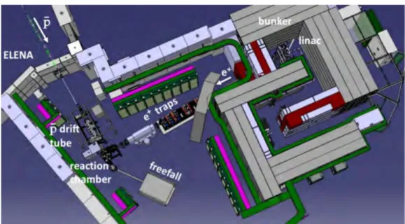
Figure 2.3 Layout of the GBAR experiment in the CERN AD hall.

Step 1 is achieved using the linac and positron traps. Step 2 is performed in parallel by the AD/ELENA rings followed by the ¯p pulsed drift tube. Step 3 is via the reaction chamber and Step 4 in the free-fall chamber. The different components are described in the following section.

(31)

2.2 Experimental setup

2.2.1 Linac and Positron source

A linac (linear accelerator) of 9.5 MeV energy and 300 mA peak current running at 300 Hz repetition rate accelerates electron bunches of a few microseconds length.

Positrons are created by impinging the electrons on a tungsten target. Some of the elec-trons interact with the target nuclei and emit high energy Bremsstrahlung rays. Gamma rays with a large enough energy can dissociate into electron-positron pairs. Considering an electron to positron conversion of K(e− _{−→ e}+_{) ∼ 10}−4_{, a 10}7 _e+_/bunch _{rate is}

ex-pected behind the target.

The high radiation requires the linac and the tungsten target to be placed in a bunker made of iron and concrete as displayed in Figure-2.3 (without roof). As illustrated in the Figure-2.4, the unusual vertical position of the assembly was chosen to limit the dose depositions.

Figure 2.4 Sketch of the linac mounted above the positron tungsten target and moderator inside the GBAR bunker [107]

Since the energy of the newly generated positron is too high, the tungsten target in-cludes a tungsten mesh moderator [108]. Positrons injected into tungsten are slowed down in the metal to thermal energy. The positrons deeply thermalized are annihilated, while the positrons reaching the surface can be re-emitted in vacuum with a few eV energy. A potential difference is applied to the moderator to define the kinetic energy of the beam for downstream transport.

The beam passes through a magnetic separator that selects only the low energy positrons (∼ 50 eV ). The beam is guided outside the bunker along a vacuum line covered with a solenoidal winding generating a axial magnetic field of 8 mT that radially confines the positrons. Finally, a buncher compresses the 2.5 m positron pulse in time to inject it into a finite-length trap cavity.

The linac was constructed for GBAR by NCBJ2 _{and installed in January 2017 and}

the first e+ _{pulses were generated in November 2017. A average preliminary flux of}

3.4 105 _e+_/bunch_{was measured.}

(32)

2.2. EXPERIMENTAL SETUP 31

Buffer-Gas Trap

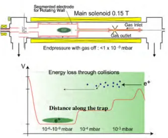
The first step of the positron stacking is carried out using a buffer gas trap (BGT ) filled with N2gas. Developed by Murphy and Surko in 1992 at the University of San Diego [109],

it consists of a 0.1 T Penning-Malmberg trap made of three stages. A scheme of a BGT is shown in Figure-2.5. Positrons are cooled by Coulomb interactions with the electrons of the N2 molecules. The design of the electrodes and of the vacuum chambers was chosen

to optimize the differential pumping. When a maximum of positron bunches have been stacked, the plasma is compressed using the rotating wall technique3_{. The latter consists}

of inducing angular momentum to the plasma in order to reduce its radius (see Ref.-[113]).

Figure 2.5 Principle scheme of the buffer gas trap. The positron are injected from the left.

Accumulation Trap

The pressure in the last cavity of the BGT is too high for positron accumulation which requires long storage time. Once the rotating wall technique applied, the positrons are sent to a cryogenic 5 T Penning-Malmberg trap. A picture of the trap is displayed in Figure-2.6. Details can be found in Refs.-[114, 115].

Figure 2.6 Picture of the positron accumulation trap.

(33)

2.2.2 Reaction Chamber

After accumulating about 1010 _{positrons, the plasma is ejected from the trap with an}

energy of about 5 keV . It is focused through electrostatic optics onto a silicon cell to produce positronium. This cell, named positron-positronium converter (PPs, also referred as reaction chamber), is a bar with an effective rectangular cross section of 1 mm2

(an-tiproton beam view) and is 20 mm-long. It is composed of silicon coated inside with nanoporous silicon oxide (SiO2). A schematic of the reaction target is shown in

Figure-2.7.

Figure 2.7 Sketch of the ¯p − P s interaction region.

Positrons extracted from the storing trap pass through a first windows made of 30 nm of silicon nitride (SiN), transparent to 5 keV positrons. Thus, they hit the opposite wall of the cell coated with SiO2. In recent years, the potential for nanoporous insulator

materials to be used as highly efficient Ps converters has been recognized and extensively studied [116]. When e+ _{are implanted into such a material at kinetic energies of a few}

keV, they scatter off atoms and electrons in the bulk and are slowed to eV-scale energies within a few ps. With efficiencies of a few tens of percent, the slow positrons capture bound electrons, which tend to accumulate in defects of the material. In the pores, Ps repeatedly bounces off the cavity walls and eventually approaches complete thermaliza-tion with the target material. Figure-2.8 shows typical scenarios for the producthermaliza-tion of positronium in the converter.

Figure 2.8 Schematic of the ortho-positronium formation principle in the PPs converter. From Ref.-[117].

Two types of positronium atoms are synthesized corresponding to the relative orien-tations of the spins of the electron and the positron. An anti-parallel spin state S = 0, called para-positronium (pPs),and a parallel spin state S = 1, called ortho-positronium

(34)

2.2. EXPERIMENTAL SETUP 33 (oPs). Both positronium states are meta-stable and annihilate after some time. The main difference between these two states is their lifetime. Para-positronium has a lifetime of almost 250 ps, and does not exist long enough to react with antiprotons. Per contra, ortho-positronium with a lifetime of approximately 150 ns is therefore more favorable to react to form antihydrogen. A 30% efficiency for oP s conversion has been measured with positrons of 3 keV and less [118, 119].

The production of H+_{ions is initiated by the injection of an antiproton pulse into the}

conversion target, via the two successive reactions Eq.-(2.2) and Eq.-(2.3).

The cross section of the first reaction was measured with its matter equivalent reaction p + P s −→ H + e− for energies of the order of 10 keV for the proton. It is estimated for lower energies in Ref.-[106]. Inversely, the cross section of the second reaction was not measured but estimated for its matter equivalent reaction H + P s −→ H − +e+ _{in the}

order of 10−16 _cm2 _[120].

The cross section of the double reaction is shown in Figures-2.1 respectively. The cross section of the second reaction can only occur for ¯H atoms with energies higher than 6 keV with ground state Ps. This cross-section increases if the positronium is in an excited state. The laser excitation of the Ps is then investigated as a serious solution to increase the ¯H+ _{production for the states n = 3 and n = 2.}

At CERN, the converter assembly and commissioning is currently in progress. Since the PPs converter is at the crossroad of the positron beam, antiproton beam and laser beams, it has to take into account the different mechanical and electromagnetic con-straints. In fact, the converter must be located downstream of the positron storing trap, away from its fringe field influence, in order to not reduce the lifetime of the oPs states [120]. At the same time, the reaction chamber has to be aligned on the antiproton path.

2.2.3 Capture, cooling and free-fall

Capture and precision traps

As detailed in Ref.-[121], ¯H+ _{ions are guided, decelerated}4 _{and captured into a RF linear}

trap using sympathetic cooling with laser cooled Be+_{ions. For this purpose, Be}+_{ions are}

loaded into the RF trap and undergo a Doppler laser cooling using UV light at 313 nm. The low-energy Be+ _{ions (∼ mK) organize by forming a Coulomb crystal, as shown in}

Figure-2.9.

Figure 2.9 Photograph of cold Be+ _{(∼ mK) crystals with 4500 ions trapped [107].}

4_{The final deceleration process is still under investigation. Hints show that a similar Pulsed Drift}

(35)

The ¯H+_{ions arriving from the side of the crystal, loose energy via coulomb interaction}

with the cooled Be+ _{ions. The light ions such as ¯}_H+ _{tend to concentrate at the center}

of the coulomb crystal when the heavier ones (Be+_{) remain on the periphery. Intensive}

simulations [122] showed that the capture efficiency of the ¯H+_{ions is enhanced using}

spe-cific mass ratios. The possibility of using an intermediate ion species such as HD+ _ions

between the Be+ _{and ¯}_H+ _{ions is under investigation. The use of such an intermediate}

species5 _{would reduce the required cooling time (according to [122] t}

capt ∝ N− 4 3 ions).

Figure 2.10 Picture of the precision trap (left), details on the cavity and x-shaped

elec-trodes of the precision trap (right). The gap between the end caps is almost 2 mm [123].

After the capture trap, the ¯H+_{trip ends in the precision trap. The latter consists of an}

x-shaped, gold coated, micro-fabricated chip trap as shown in Figure-2.10. The x-shaped chips provide a RF trapping field for radial confinement and two DC endcaps for longitu-dinal confinement. In the trap cavity, Raman sideband cooling is applied, preparing the

¯

H+ _{ions in the vibrational ground state at ∼ 10 µK (respectively : ∼ 1 neV energy). At}

the end of all the successive cooling processes, the velocity dispersion of the ¯H+ _{ions is}

expected of the order of 1 m/s.

Finally, a quasi-at rest ¯H atoms are obtained by photo-detaching the excess positron of the ¯H+ _{ions. The laser pulse generating the excess positron ejection, initiates the}

free-fall time measurement. Free-fall detection

The capture and precision traps are maintained inside a detection chamber. The design of which is shown in Figure-2.11. A small electrostatic quadruple bender deviates the beam, transported from the reaction chamber, with a 90◦ _{angle. This chamber has been}

designed to sustain UVH vacuum, a homogeneous low magnetic field required for Raman cooling and a high radiation transparency. The chamber is about 1 m tall.

The free-fall is initiated with the photo-detachment laser. The newly produced ¯H atoms fall into the chamber and annihilate hitting the bottom plate of the chamber. The chamber is surrounded by several layers of detectors. They detect the position and time of the exiting pions coming from the annihilation of the antiprotons.

Two types of detectors are used. The first ones are Micromegas-type gaseous detectors. Such detectors have a high spatial resolution, but a low time resolution. Three layers

(36)

2.2. EXPERIMENTAL SETUP 35

Figure 2.11 Sketch of the free-fall chamber housing the capture and precision traps. The Raman laser beams, the magnetic shielding and the cryo-cooling system are indi-cated [124].

of Micromegas detector are used to reconstruct the path of the pions to localize the annihilation position. The second are plastic scintillators, with a low spatial resolution but with a high time resolution. These detectors are used to trigger the passage of the pions and reconstruct the free-fall time considering the pion time-of-flight delay. The high resolution of the plastic scintillator allows removing background events such as cosmic rays.

2.2.4 Antiproton decelerator (this thesis)

While the positron beams are being prepared, the ¯p are being decelerated in the AD/ELENA to 100 keV .

In the experimental proposal [94], the GBAR collaboration accepted an innovating electrostatic decelerating system whose central element is a Pulsed Drift Tube (PDT ) decelerating the ion bunches and selecting the downstream energy of the beam. Such a deceleration technique for antimatter has been mentioned for the very first time by Nieto and Goldman in reference-[125].

Figure 2.12 Principle scheme of the GBAR decelerator.

Transported at ground potential, the antiproton pulse slows down facing the strong electric field at the entrance of the drift tube. Passing though it, particles reach a local

Deceleration of antiprotons from CERN’s ELENA synchrotron and transport of antimatter beams through the GBAR experiment

HAL Id: tel-02526874

https://tel.archives-ouvertes.fr/tel-02526874

Submitted on 31 Mar 2020

HAL is a multi-disciplinary open access

archive for the deposit and dissemination of

sci-entific research documents, whether they are

pub-lished or not. The documents may come from

teaching and research institutions in France or

abroad, or from public or private research centers.

L’archive ouverte pluridisciplinaire HAL, est

destinée au dépôt et à la diffusion de documents

scientifiques de niveau recherche, publiés ou non,

émanant des établissements d’enseignement et de

recherche français ou étrangers, des laboratoires

publics ou privés.

synchrotron and transport of antimatter beams through

the GBAR experiment

Audric Husson

To cite this version:

Audric Husson. Deceleration of antiprotons from CERN’s ELENA synchrotron and transport of

antimatter beams through the GBAR experiment. General Relativity and Quantum Cosmology

[gr-qc]. Universite Paris Saclay, 2018. English. �tel-02526874�

NNT

:2018SA

CLS255

Deceleration of antiprotons from CERN’s

ELENA synchrotron and transport of

antimatter beams through the GBAR

experiment

A

UDRIC

HUSSON

Contents

List of Figures

List of Tables

Chapter 1

Introduction

1.1

Antimatter discovery

1.1.1

Dirac equation and the negative solution problem

1.1.2

From theory to experiment : antimatter under the spotlight

1.2

(anti-)atoms in an (anti-)Universe

1.3

"Defying gravity"

1.3.1

The (not so) Weak Equivalence Principle

1.3.2

From theory to experiment

1.4

What about antigravity ?

1.4.1

Indirect estimation

1.4.2

Astronomical observations

1.4.3

Direct attempts

1.5

Toward current experiments

1.6

How to decelerate a beam (further)?

1.7

This thesis

Chapter 2

The GBAR experiment

2.1

Principle

2.2

Experimental setup

2.2.1

Linac and Positron source

2.2.2

Reaction Chamber

2.2.3

Capture, cooling and free-fall

2.2.4

Antiproton decelerator (this thesis)