Computational Modeling of a Hall Thruster
Plasma Plume in a Vacuum Tank
by
Shannon Yun-Minug
C
heng
Submitted to the Department of Aeronautics and Astronautics
in partial fulfillment of the requirements for the degree of
Master of Science in Aeronautics and Astronautics
at the
MASSACHUSETTS INSTITUTE OF TECHNOLOGY
February 2002
@
Massachusetts Institute of Technology 2002. All rights reserved.
A u th o r ...
Department of Aeronautics and Astronautics
February 1, 2002
C ertified by ...
Manuel Martinez-Sanchez
Professor
Thesis Supervisor
A ccepted by ...
Wallace E. Vander Velde
Professor of Aeronautics and Astronautics
Chair, Committee on Graduate Students
Computational Modeling of a Hall Thruster Plasma Plume
in a Vacuum Tank
)y
Shannon Yun-Ming Cheng
Submitted to the Department of Aeronautics and Astronautics
on February 1, 2002., in partial fulfillment of the
requirements for the degree of
Master of Science in Aeronautics and Astronautics
Abstract
Hall thrusters have become a tempting alternative to traditional chemical propulsion
systems due to the great mass savings they provide through high specific impulses.
However, a major stumbling block to their widespread integration is uncertainty about
the thruster plume's interaction with spacecraft components. While in-space data is
difficult to collect, much experimental data from vacuum tank tests is readily
avail-able. Effectively taking advantage of this wealth requires understanding of the effects
from imperfect ground test conditions. A previous plume model,
Qasi3,
has been
upgraded to better simulate the vacuum tank environment primarily through
improve-ments to the source model, the collision method, and the sputtering method. The
code is now more accurate and provides insight into phenomena such as background
pressure consequences. sputtering and sputtered material deposition.
Thesis Supervisor: Manuel Martinez-Sanchez
Title: Professor
Acknowledgments
I would like to thank my advisor, Professor Martinez-Sanchez, for both his great
patience and his enthusiasm. An open door always greets me and my incessant
questions, regardless of time of day or the huge piles of other work he has. His
genuine interest and curiosity in my work is contagious and keeps me motivated and excited about research.
Thanks are also in order for my whole family - Mom, Dad, Serena, and Adrian.
They all possess that wonderful gift of being able to raise my spirits even from
thou-sands of miles away, and I hope they know how much they mean to me.
I owe a great debt to Mike Fife for sending me the original version of Quasi3 and
helping me get HPHaUI working with the BHT-200 grid. I literally wouldn't have gotten anywhere with my research without his help.
One of the great perks of being a student is all the cool people you get to hang out with. Thank you to everyone in SPL -- Tatsuo. Paulo, Luis Fernando, Jorge, Vincent, Anne, and Murat - for helping me whenever I need it, making the lab a fun environment to come and work in, and generally enhancing grad student life. Thank you to my roommates, Andrew, Chris, and Gong Ke, for understanding when I wasn't around much, giving me great advice, and always making me smile. Special
thanks to Raffi, Jessica, and Ethan for all the moral support and for bailing me out of numerous computer troubles. And thank you to Al and Julie for getting me through the last month.
Last, but certainly not least, thank you to Leo and Pinky for being with me from the very beginning and never once complaining.
Contents
1 Introduction
19
1.1
Hall Thrusters . . . .
19
1.2 Motivation.... .... ... 19
1.2.1 Advantage of Electric Propulsion . . . . 19
1.2.2 Hall Thruster Integration Issues . . . . 20
1.2.3
ET EEV . . . .
22
1.3 Outline of Research . . . .
23
2 Original Plume Model 25 2.1
Q
uasi3 . . . . 252.1.1 PIC method . . . . 25
2.1.2 Collision Model . . . . 27
2.1.3 Computational Grid . . . . 27
2.1.4 Source Model . . . . 28
2.1.5 Surface Interaction Model . . . . 30
2.2 Later Modifications to Quasi3 . . . . 31
2.3 Starting Point of this Research . . . . 32
3 Source Model 33 3.1 O verview . . . . 33
3.2 Prelininary Source Model . . . . 35
3.2.1 Exit Plane Distributions . . . . 39
3.3
Improved Source Model
.
. . . .
3.3.1 Exit Plane Distributions . . . .
3.3.2 Additional parameters . . . .
3.4 Comparison of Source Models . . . .
4 Collisons
4.1 Overview. . . . . 4.2 Charge Exchange Cross-section . . . . 4.3 Elastic collisions . . . . 4.4 Neutral weighting selection . . . .
5 Sputtering
5.1 Overview. . . . . 5.2 Normal Sputtering Yield . . . . 5.3 Angular Dependence of Sputtering Yield . . .
5.4 Low-energy Sputtering Method . . . .
5.5 Angular Distribution of Sputtered Material . 5.6 Implementation of Sputtering Method . . . . .
44
46
71
71
75
75
75
76
78
81
81
82
84
88
88
92
6 Results and Conclusion 95
6.1 O verview . . . . 95
6.2 Current Density Distribution . . . . 95
6.2.1 Comparison to Experimental Data . . . . 99
6.2.2 Effect of Background Pressure . . . . 100
6.3 Simulation in Vacuum Tank . . . . 114
6.3.1 Simulation Geometry . . . . 114
6.3.2 Tank Simulation Results . . . . 118
6.3.3
Tank Filling ...
.
...
...
135
6.4 Sources of Error . . . . 135
6.4.1 Charge Exchange . . . . 135 142
6.4.3
Lack of Experimental Data . . . .
144
6.5 Conclusions . . . . 146
6.6 Future Work . . . .
146
A Other Code Modifications 149
A.1
Sheath Model . . . .
149
A.1.1 Sheath Drop . . . . 149
A.1.2 Conducting Surface Sheaths . . . . 150
A.2 Potential Reference Method . . . . 151
A.3 Visualization Software . . . . 152
B Quasi3 Manual 153 B.1 Overview . . . . 153
B .2 M esh3 . . . . 154
B.3
Quasi3
. . . .
162
B.4 Visualization Software . . . . 164
List of Figures
1-1 Cross-section of typical Hall thruster. . . . . 20
2-1 Particle-In-Cell (PIC) methodology. . . . . 26
2-2 Experimental measurements of near-field current density. [6] . . . . . 30
3-1 B H T-200. . . . .
34
3-2 Spatial grid for the BHT-200 geometry. . . . . 36
3-3 Side view of BHT-200. . . . .
37
3-4 Simulated performance of BHT-200 from Hall. . . . .
38
3-5 Space potential for BHT-200. . . . .
38
3-6 Simulated Xe+ flux. . . . .
40
3-7 Modeling of BHT-200 exit plane. . . . . 41
3-8 Calculation of azimuthal ion drift velocity. . . . . 43
3-9 Simulated performance of BHT-200 from HPHall. . . . . 45
3-10 Exit plane for improved source model. . . . . 46
3-11 Xenon single ion axial velocity distributions. Horizontal axes are axial velocity, vz, ranging from 0 to 35000 m/s. Vertical axes are number of Xe+ ranging from 0 to 3 x 10². . . . . 47
3-12 Xenon single ion radial velocity distributions. Horizontal axes are
ra-dial velocity, v, ranging from -35000 to 35000n/s.
Vertical axes are number of Xe+ ranging from 0 to 4 x 10¹². . . . . 483-13 Derivation of Xet number density distribution.
. . . .
49
3-14 Split of single ion populations. . . . .
50
3-16 Near-side population single ion axial velocity distributions. Horizontal
axes are axial velocity, v,. ranging from 0 to 35000 rn/s. Vertical axes
are number of near-side Xe+ ranging from 0 to 3 x 10². . . . . 52
3-17 Near-side population single ion radial velocity distributions. Horizontal axes are radial velocity, v,, ranging from -35000 to 35000 m/s. Vertical axes are number of near-side Xe+ ranging from 0 to 4 x 10¹². . . . . . 53
3-18 Axial near-side ion temperature. . . . . 54
3-19 Single ion far-side population velocity distributions. . . . . 55
3-20 Far-side population single ion axial velocity distributions. Horizontal axes are axial velocity, v,. ranging from 0 to 35000 m/s. Vertical axes are number of far-side Xe+ ranging from 0 to 1 x 10¹². . . . . 57
3-21 Far-side population single ion radial velocity distributions. Horizontal axes are radial velocity, v,, ranging from -35000 to 35000 m/s. Vertical axes are number of far-side Xe+ ranging from 0 to 2 x 10¹² . . . . . . 58
3-22 Axial far-side ion temperature. . . . . 59
3-23 Derivation of Xe++ number density distribution. . . . . 61
3-24 Split of double ion populations. . . . . 62
3-25 Double ion near-side population velocity distributions. . . . . 63
3-26 Near-side population double ion axial velocity distributions. Horizontal axes are axial velocity, v., ranging from 0 to 35000
n/s.
Vertical axes are number of near-side Xe++ ranging from 0 to 3 x 101. . . . . 643-27 Near-side population double ion radial velocity distributions. Hori-zontal axes are radial velocity, v,, ranging from -35000 to 35000 m/s. Vertical axes are numuber of near-side Xe++ ranging from 0 to 4 x 10". 65 3-28 Axial near-side double ion temperature. . . . . 66
3-29 Double ion far-side population velocity distributions. . . . . 67
3-30 Far-side population double ion axial velocity distributions. Horizontal axes are axial velocity, v., ranging from 0 to 35000
n/s.
Vertical axes are number of far-side Xe++ ranging from 0 to 1 x 10.. . . . . 683-31 Far-side population double ion radial velocity distributions. Horizontal
axes are radial velocity, Vr ranging from -35000 to 35000 m/s. Vertical
axes are number of far-side Xe++ ranging from 0 to 15 x 1010.
3-32 Axial far-side double ion temperature.
. . . .
3-33 Comparison of source models
-
single ions. . . . .
3-34 Comparison of source models
-
double ions. . . . .
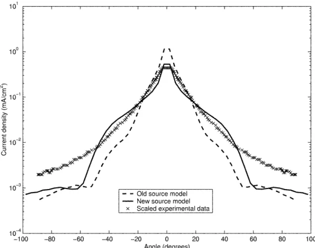
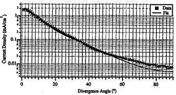
3-35 Comparison of source models. . . . .
3-36 Ion current density versus divergence angle, measurements scaled to 1
m radius from the thruster exit plane. [12] . . . .
4-1 Simulated retarding potential analyzer (RPA) measurements for P
5
x10
-T ori.. . . . .
Normal incidence sputtering yield for silicon by xenon. . . . . Sputtering yield of silicon by incident xenon at 200 eV. . . . . Dominant sputtering mechanism near normal incidence. . . . . Dominant sputtering mechanism at oblique incidence. . . . . Sputtering yield of silicon by xenon for various incident angles... Near-threshold energy sputtering curves for xenon strikinig silicon. Sputtering angles. . . . . Angular distribution of sputtered material for E/E, = 2. . . . .
3D view of current density simulation domain. . . . .
Embedded meshes for current density simulation domain... Comparison of current density distributions in vacuum. . . . . . Comparison of scaled and simulated data. at 60 cm. . . . . Current density distributions for various background pressures at Simulated RPA data at 70' for various background pressures. . . Velocity phase-space plot for single ions. . . . . Velocity phase-space plot for double ions. . . . . Charge exchange ions for different background pressures...
. . .
96
. . .
97
. . .
98
. . .
99
60 cm.100
. . .
101
. . .
102
. . .
103
. . .
104
5-1 5-2 5-3 5-45-5
5-6
5-75-8
6-1 6-2 6-3 6-46-5
6-6
6-7
6-86-9
6-10 Source ions for different background pressures . . . . . 6-11 Current density distributions for various background pressures at 60
crn, with inclusion and exclusion of source neutrals. . . . .
6-12 Current density
[mA/cm
2]
versus background pressure[Torr] at
vari-ous angles. Solid line represents current density at P = 0 Torr. Dashed
line represents current density without source neutrals at P = 0 Torr.
6-13 Current density
[mA/cm
2]
versus background pressure [Torr] at
vari-ous angles. Solid line represents current density at P = 0 Torr. Dashed
line represents current density without source neutrals at P
=
0 Torr.
6-14 Current density
[mA/cm
2]
versus background pressure [Torr] at
vari-ous angles. Solid line represents current density at P = 0 Torr. Dashed
line represents current density without source neutrals at P
=
0 Torr.
6-15 Fractional split of source and CEX ions versus background pressure
[Torr] for various angles. Horizontal axis is pressure from 0 to 4x 10⁻⁵
T or.. . . .
6-16 Fractional split of source and CEX ions versus background pressure
[Torr] for various angles. Horizontal axis is pressure from 0 to 4x
10-T orn.. . . .
6-17 Fractional split of source and CEX ions versus background pressure
[Torr] for various angles. Horizontal axis is pressure from 0 to 4x 10⁻⁵
T orr. . . .
6-18
6-19
6-20
6-21
6-22
6-23
6-24
6-25
6-26
Simulated tank geometry. . . . .
115
Witness plate orientation (top view). . . . . 116
Witness plate orientation (back view). . . . . 117
Xe particles after 1000 iterations. . . . . 119
Xe particles after 1000 iterations. . . . .
120
Witness plate 1, west wall, silver material. . . . .
123
Witness plate 1, east wall, silver material. . . . .
124
Witness plate 2, west wall, silver material. . . . .
125
Witness plate 2, east wall, silver material. . . . .
126
105
107
108
109 110 111 112113
6-27
6-28
6-29
6-30
6-31
6-32
6-33
6-34
6-35
6-36
6-37
6-38
6-39 Xe
-
Xe++ CEX rate [1/m
3/s].
Region used to estimate
inissing
CEX from source model. Effect of electron temperature. . . . .HPHall exit plane averages. . . . .
Average potential in cross-section of plume. . . . .
A-1 Sheath drop. . . . .
East wall, iron material. . . . .
North wall, iron material.
. . . .
Up wall, iron material. . . . .
West wall, iron material. . . . . Up wall, iron material. . . . .
West wall, iron material. . . . . Up wall with background density, iron material.
West wall with background density, iron material.
Particle totals for tank filling case.
. . . .
Species temperatures for tank filling case . . . . . Species pressures for tank filling case. . . . .Xe -Xe+
CEX
rate[1/m3]
...6-40
6-41
6-426-43
127
128
129
130
131
132
133
134
136
137
138
140
140
141
143
144
145
150
.
.
.
.
List of Tables
2.1
Collisions simulated in Quasi3.. . . . .
2.2 SPT-100 nominal operating parameters. . . . .
2.3
Source model parameters for SPT-100. . . . .
3.1 BHT-200 nominal operating parameters. . . . . 3.2 Simulated performance of BHT-200 from Hall.. . . . . 3.3 Preliminary BHT-200 source model parameters. . . . . 3.4 Simulated performance of BHT-200 from HPHall. . . . . 3.5 Improved BHT-200 source model parameters. . . . .
5.1 Sputtering yield calculation parameters with Xe as the projectile. 5.2 Sputtering yield thresholds. . . . .
28 29
29
3335
44 4571
85
88
6.1
CEX production rates in
engine region before exit plane. . . . . 141 6.2 CEX production rates in plume region for various background pressures. 142B.1
B.2
B.3
B.4
B.5
Variables in a .in file. . . . . . Quasi3 switches. . . . .
Mesh 3
switches. . . . . Changes to Mesh3. . . . . Changes in Quasi3. . . . .. . . .
1 6 3
. . . . 1 6 3. . . .
1 6 3
. . . . 1 6 6. . . .
1 6 7
Chapter 1
Introduction
1.1
Hall Thrusters
Hall thrusters are members of the electric propulsion family, characterized by an an-nular acceleration channel and a radial magnetic field. Electrons are emitted from an external cathode and backstream towards the anode where they encounter the mag-netic field. Because of their small Larmor radius and long collision mean free path, electrons are prevented from diffusing across the magnetic field easily and are effec-tively captured in azimuthal drifts along field lines. Neutral propellant gas, typically xenon, is injected into the channel near the anode and undergoes ionization upon contact with the trapped electrons. The resultant heavy ions have a Larmor radius much larger than the thruster's dimensions and are accelerated out of the channel by the axial electric field with little influence from the magnetic field. Figure 1-1 shows the cross-section of a typical Hall thruster.
1.2
Motivation
1.2.1
Advantage of Electric Propulsion
Hall thrusters and other types of electric propulsion have recently attracted much interest as they provide high specific impulses at relatively high efficiencies. Unlike
Cathode
Anode
|Magnet
Centerline Magnet
Figure 1-1: Cross-section of typical Hall thruster.
conventional chemical propulsion systems, electric propulsion devices do not rely on the internal energy stored within their propellant. Instead, an external power source
is used to impart energy to the working fluid. As no inherent limitation due to
the propellant exists, a high Ip is attainable which translates to a highly desirable
mass savings. Higher exhaust velocities and thus higher specific impulses are only
constrained by the power processing unit (PPU) which provides the external energy
and is the primary contributor to the electric propulsion system's mass. By balancing ,p with PPU mass, Hall thrusters are found to fall in an optimum operation regime
well-suited for missions such as station-keeping and orbit transfers.
1.2.2
Hall Thruster Integration Issues
Despite numerous advantages, reservations about integrating Hall thruster technology into space systems exist because of various unknowns. One large area of concern
is the interaction the thruster plume has with the spacecraft. As a result, many
efforts have been made to study these effects through both experiment and simulation. To date, very little in-space plume data has been taken as such experiments are both difficult and expensive. Conversely, a multitude of vacuum tank experiments
have been performed or are planned for the near future. While these on-ground tests provide much insight into the behavior of the Hall thruster and its plume, interpretation of the collected data also needs to take into account effects due to imperfect experimental conditions.
One such limitation is the finite capability of the vacuum pumps. Because per-feet vacuum conditions cannot be achieved, a nominal background neutral density exists that interacts with the plume through collisions. While ionizing collisions with these background neutrals cause an increase in measured thrust if ions are created at higher than background potential, the effects of charge exchange (CEX) collisions are of greater concern. These collisions occur when the positive charge of a fast-moving source ion is given to a slow-moving background neutral in a resonant process, result-ing in a high-energy neutral and a low-energy ion. The potential hump of the plume is not as easily overcome by these CEX ions and they are pushed laterally more than their energetic source ion counterparts. This phenomenon is reflected in higher values of current density at outlying angles of the distribution.
An unwanted consequence of CEX ions, whether formed from interaction with a source or a background neutral, is sputtering of objects in contact with the plume. To avoid direct impingement by the plume on spacecraft components such a s solar arrays, thrusters are generally canted at an angle. Although the thrust vector is no longer ideally aligned, the main beam is now diverted away from the sensitive surfaces. Unfortunately, though the lower energy CEX ions have less potential to cause harm, their location in the wings of the plume puts them dangerously close to the spacecraft components trying to be avoided. Some CEX ions may even be accelerated backwards and strike the spacecraft's main body. While it is hoped that damage on-orbit is kept to a minimum, it is difficult to discern its magnitude from
ground experiments. Separating the effects of a background neutral density and its subsequent elevation of CEX ion levels is not a simple task. Another integration issue is foreign material from the thruster itself depositing on sensitive spacecraft surfaces. In this case, the closed environment of the vacuum tank is an additional drawback as sputtering off of facility walls and instruments may be confused with that from the
engine.
The combination of a contained environment and the limited pumping capability causes recirculation of plasma. Plasma that would normally be dispersed in the vacuum of space is retained and may induce unexpected effects in the testing domain.
Due to these uncertainties, drawing conclusions on in-space plume behavior based on vacuum tank experiments is difficult. The goal of this research is to improve the ability of a numerical plume simulation to model a tank environment. If tank effects on thruster operation can be accurately captured by the physics of a simulation and verified against available empirical data taken on the ground, then greater confidence in the projections of the pluine's response in a perfect vacuum is earned. Furthermore,
the model then can act as a tool for correlation between the plume's behavior on
ground and in actual orbital conditions, aiding in integration of the thruster into
spacecraft.
1.2.3
ETEEV
The Electric Thruster Environmental Effects Verification (ETEEV) experiment is a
joint effort underway between MIT, WPI, Draper Laboratory, Busek, and the Air
Force Research Laboratory. The purpose of the project is to collect in-space plume
behavior of a Hall thruster and a Pulsed Plasma thruster as a Shuttle Hitchhiker
payload scheduled to fly in 2003. More detail about the experiment can be found in
the work of Thomas and Pacros [18, 11].
Design of the Hall thruster side of the experiment is being handled by MIT. A
BHT-200 provided by Busek is currently being prepared for the flight in a vacuum
tank at MIT. This research focuses on simulating the ETEEV setup as better
under-standing of the plume aids in experiment design matters such as instrument selection
and placement. A reciprocal benefit exists in that both on-ground vacuum tank and
in-space plume data will be available in the near future for code verification.
1.3
Outline of Research
This research begins with an existing numerical plume model which is then upgraded
to better simulate plumes in a tank environment. Chapter 2 gives an overview of the state of the original plume model prior to any changes. Chapter 3 describes the development of better source models to simulate the BHT-200. Chapter 4 presents efforts made to improve modeling of collisions. Chapter 5 covers enhancements to the sputtering methodology. Chapter 6 presents results and conclusions about the research. Finally, additional code modifications and a brief user's manual of the
Chapter 2
Original Plume Model
2.1
Quasi3
Quasi3 is a hybrid PIC-DSMC three-dimensional simulation of a Hall thruster plasma
plume written by Oh [10]. Expansion of the plume is modeled in a user-specified geom-etry and background pressure. Estimates of surface erosion rates for three materials are calculated based on incident particle flux and energy. Contour plots of these rates, particle fluxes and energies on simulation surfaces, and the current density distribution are the main results extracted from the simulation.
2.1.1
PIC method
Particle-In-Cell (PIC) methods treat gases as a collection of particles. Simulated
particles represent a much larger number of real particles and are referred to as macroparticles. In the case of a plasma, several species must be accounted for ions, neutrals, and electrons. Macroparticles representing these species move throughout a computational grid. At each time step, trajectories are altered due to self-induced and externally applied force fields. For a plasma, the self-induced electric field is calculated by weighting charged species to the grid nodes to determine the local charge density as in Figure 2-1. Poisson's equation,
0
00
e
0
0
0
0
0
0
00*0
0
0
0
0
Figure 2-1: Particle-In-Cell (PIC) methodology.
V 20(X., Y) y, z) ,(2.1)
is then solved on the grid and the resulting potential is differentiated to yield the
electric field,
E = -Vb.
(2.2)
Fields are weighted back to macroparticles and the resultant forces are used in in-tegration of the equations of motion to move the macroparticles to their positions for the next time step. This procedure is repeated until the total simulation tine is reached.
Quasi3
uses a hybrid-PIC methodology in which the electrons are modeled as afluid instead of as particles. Further simplification is achieved by assuming quasi-neutrality and reducing the general electron momentum equation to the Boltzmann relationship,
n, = noe kTe
(2.3)
modeled. Xenon ions are weighted to the computational grid and the resulting local
ion charge density is equated to the electron charge density because of quasi-neutrality,
*ni
ne.
(2.4)
In this manner. solving of Equation 2.1 is avoided. Equation 2.3 can then be solved for
the potential with an assumed constant electron temperature of 2 eV throughout the
plume. The electric field is calculated with Equation 2.2 and particle positions and
velocities are updated due to the resultant forces as in the traditional PIC method.
2.1.2
Collision Model
In addition to the electric field, collisions also affect macroparticle motion. A Direct
Simulation Monte Carlo (DSMC) method is used to model the collisions listed in
Ta-ble 2.1. During each iteration, a global time counter is incremented by the simulation
time step. Collisions are then performed on a cell-by-cell basis in which pairs of
colli-sion partners are selected randomly. Each cell is stepped through and if a minimum
number of particles is not within the cell, collisionality is deemed improbable, the
local time counter is incremented by the time step, and the next cell is proceeded
to. If collisions are likely, two particles are chosen randomly and undergo a
selection-rejection scheme to determine whether the collision occurs or not. If a collison occurs,
the collision frequency for that process is inverted and used to increment the local
time counter. A multi-species time counter that supports multiple collision species
and types and variable macroparticle weighting calculates this time step. The
veloc-ities of particles involved in the collision are then altered based on the collision type.
This process repeats until the local time counter exceeds the global time counter at
which point the simulation continues to the next cell.
2.1.3
Computational Grid
The entire simulation is performed on a Cartesian grid generated by a program called
Charge Exchange Elastic
Xe-Xe+ Xe-Xe+
Xe-Xe++ Xe-Xe++
Xe-Xe
Table 2.1: Collisions simulated in Quasi3.
the parent and embedded meshes used in the hybrid-PIC and DSMC routines. Em-bedded meshes are used to obtain finer resolution in areas of interest in the domain. Simulation objects such as the thruster, tank walls, or solar arrays are also included in the grid. Because a Cartesian grid is used throughout, meshes and objects are constrained to being rectangular in shape.
2.1.4
Source Model
The original source model represents the plasma flow from a SPT-100 thruster which has nominal operating parameters as summarized in Table 2.2. This plasma is
com-posed of ions, neutrals, and electrons. Since electrons are described by a simplified fluid model, source electrons are not modeled directly and are accounted for by the
Boltzmann equation. Table 2.3 summarizes source model parameters which are used along with those in Table 2.2 to calculate number fluxes of source ions and neutrals
using,
hi = ' Ifall., (2.5)
h,
=mfir(1
-
mi).
(2.6)
At each iteration, these rates and the time step determine the number of particles to be inserted into the simulation. An empirical model of the thruster's exit plane ion distribution is constructed from experimental measurements of near-field current density of a SPT thruster taken by Gavryushin and Kim [6]. The magnitude and direction of ion flow as a function of radial position are extracted from Figure 2-2 and fitted to high-order polynomials.
Specific Impulse, Is, 1610 s
Anode Specific Impulse 1735 s
Thrust 84.9 ,mN
Discharge Voltage, VI) 300 V
Discharge Current. I, 4.5 A
Propellant Flow Rate, rh 5.0 mg/s
Propellant Fraction to Cathode 7.5%
Table 2.2: SPT-100 nominal operating parameters.
Exit Plane Outer Radius, r
10.100 m
Exit Plane Inner Radius, r2 0.056 m
Anode Propellant Fraction,
f,
0.929Anode Utilization Fraction, 7, 0.95
Cathode Orifice Radius 0.0005 m
Cathode Axial Offset 0.01 "?
Cathode Radial Offset
0.075 To
Xe+ Axial Drift Velocity
17,020 mr/s
Xe+ Azimuthal Drift Velocity
250.0 mn/s
Xe+ Axial Temperature
34 cV
Xe+ Radial Temperature
0.689655172 eV
Xe+ Azimuthal Temperature
0.068975517 eV
Xe Temperature
0.086 eV
Figure 2-2: Experimental measurements of near-field current density. [6]
The magnitude of the current density is converted to a number density by assum-ing all ions are sassum-ingly-charged and leave the thruster with a drift velocity of 17,020
m/s. This number density is integrated across the exit plane to find total ion flow and
then normalized, resulting in a probability distribution. Integrating this result gives a radial cumulative distribution function which decides where particles are injected radially. The direction of the current density vectors are used to derive a beam di-vergence angle function to choose what direction to insert particles in. The assumed drift speed of 17,020 m/s is broken into radial and axial components based on the divergence angle. At each time step, the number of charged particles to be inserted is calculated with Equation 2.5 and a user-specifed fraction is assumed to be doubly ionized. Double ions are assumed to have the same distribution as the single ions and are injected in the same manner, the only difference being their double charge.
2.1.5
Surface Interaction Model
A crude surface interaction model predicts erosion of material off object surfaces
in the simulation. When particles cross a cell boundary, the boundary type is de-termined from the information stored in the grid. If the boundary corresponds to an object boundary, sputtering due to the particle impact is calculated. Because quasi-neutrality is assumed in the model, resolution of the non-quasi-neutral sheath boundary is not accomplished. Thus, a sheath interaction model is used to account for this region. Typically, the object surface will fioat negative with respect to the
pre-sheath plasma potential, causing positively charged ions to be accelerated towards the wall. The potential drop across the sheath is calculated with,
k ITe 4I
(2.7)
C .necej
Energy due to acceleration through this sheath potential is added to the particle impacting the object surface. This energy is then used to calculate the sputtering yield of silver, quartz, and silicon from fits to experimental sputtering data. These fits are linear relationships between sputtering yield and incident particle energy generated from data for normally-incident particles. Sputtering yields are then translated to erosion rates for each material and averaged over the duration of the simulation. Ions striking surfaces are deleted from the simulation while neutrals are reflected
specularly.
2.2
Later Modifications to Quasi3
Since its completion, Oh's work has been expanded upon. In studying issues related to integrating a Hall thruster acceleration channel model with Quasi3, Qarnain [13] modified the original source model. Fifes [5] hybrid PIC-MCC two-dimensional en-gine code, Hall, is used to generate a simulated exit plane current density distribution from which cumulative radial distribution and beam divergence angle functions are derived. The source models axial ion temperature is also changed from 34 cV to 3.4 eV. Oh had originally chosen 34 eV because this value seemed to give better results for the current density distribution. However, experimental as well as sim-ulated results of ion energy distributions point toward a value smaller by an order of magnitude. Further modification to Quasi3 includes improvement on the surface interaction model by incorporating an empirical model for angular dependence of
sputtering yield developed by Yamamura et. al [20]. This model introduces an inci-dent angle-depeninci-dent correction factor to the normal sputtering yield calculated in
Oh's original surface model.
Ya-mamura method for angular dependence of sputtering yield is retained. However, calculation of the normal sputtering yield is performed with a formulation by
Mat-sunamin, recommended by Yamanmura. In addition to tabulating the erosion rates of surfaces, the sputtering yield is also used to insert sputtered particles into the sim-ulation. These particles are tracked throughout the domain and their subsequent deposition on other objects is recorded. Parameters for xenon sputtering aluminum are used to calculate yields, so all objects are effectively composed of aluminum. Alu-minum particles are ejected from the surface in-plane at 450 and travel on straight-line trajectories until they either impact another surface or leave the simulation via am exterior boundary. Incident particles striking surfaces are reflected with 80% of their original energy and incident ions are neutralized before reflection.
2.3
Starting Point of this Research
Unfortunately, while trying to port Quasi3 from a UNIX to a PC system, the version with the later modifications did not run properly. Thus, the original version of the code written by Oh was procured and serves as the starting point of this research.
Chapter 3
Source Model
3.1
Overview
The
Quasi3
source model is of utmost importance in achieving good plume simulation
results. The source model encapsulates the state of the plasma exiting the Hall
thruster and must be detailed if accurate results of its expansion as a plume are
desired. Past work with Quasi3 has used a SPT-100 source model derived either from experimental data or from results of a computational simulation. For this work, the source model is of the lower power Hall thruster being used for the ETEEV experiment, the BHT-200. The thruster is pictured in Figure 3-1 and its nominal operating parameters are summarized in Table 3.1.
Anode Specific Impulse 1530 s
Thrust 10.5 mN
Discharge Voltage, V0 300 V
Discharge Current, 1, 0.65 A
Thruster Mass Flow Rate, ith 0.70 mg/s Cathode Mass Flow Rate, rh, 0.10 mg/s
3.2
Preliminary Source Model
A preliminary BHT-200 source model is generated in the same way that Qarnain
developed a computational SPT-100 source model. Fife's engine code, Hall, had
previously been regridded as in Figure 3-2 to simulate the BHT-200 by Szabo [17].
Figure 3-3 shows a schematic of the side view of the BHT-200. The rounded tip
can be seen in the curved portion of the
bottom
of the computational grid which
corresponds to the thruster centerline. The left-hand curve of the grid represents a
"virtual anode," corresponding to the first magnetic streamline that intersects the
an-ode. Electrons are expected to flow directly down this streamline into the anode since
their mobility parallel to the magnetic field is much greater than in the perpendicular
direction. Consequently, the thruster channel upstream of this streamline is
domni-nated by neutrals since electrons are not present to cause ionization and is ignored
by the simulation. If the grid is rotated about the centerline, the annular BHT-200 is
obtained. Runs are performed over several thruster oscillations and time-averaged to
provide exit plane information for the new Quasi3 BHT-200 source model. Simulated
thruster performance parameters from Hall are shown in Figure 3-4 and Table 3.2.
The exit plane location is chosen at z = .030 m since the space potential as seen in
Figure 3-5 has mostly fallen off by the time ions reach this axial position. As Quasi3
does not directly model ions falling through the potential produced by the thruster,
it is important that these effects are already incorporated into the source model.
Thrust, (F)
10.0 mN
Anode Current, (Ia)
0.6821 A
Beam Current, (Ib) 0.4424 A
0I2 I I I iI I I 0.02-0.015 0.01 0.005 0--0.005 I I I I I 0 0.005 0.01 0.015 0.02 0.025 0.03 0.035 0.04 0.045 z(m)
Figure 3-2: Spatial grid for the BHT-200 geometry.
K B= 0.25, V0 = 300 V, simple wall conditions .5-0 0 0.5 1 1.5 2 2. 1x 10-, .5q. k&,A&I, " " 1 "Lj 00V0
~
F il 0 0 0.5 0.5 time (s) 1.5 1.5 2 2Figure 3-4: Simulated performance of BHT-200 from Hall.
0.025 r-0 0.005 0.01 0.015 0.02 0.025
z(m)
U.Ua) U.UJO phi (V) 278.878 260.282 241.685 223.089 204.492 185.895 167.299 148.702 130.106 111.509 92.9123 74.3157 55.7191 37.1225 18.5259 0.04 0.045Figure 3-5: Space potential for BHT-200.
0 0) E -0 (If ('2 0.015 Z 0.01 0.005 I. 2.5 x 10⁴ 2.5 x 10~, 0.02 0.015
E
0.01 0.005 0 1 1,1160101111114"ill MTPW"?-" ' T 13.2.1
Exit Plane Distributions
Figure 3-6 shows the averaged simulated Xe+ flux. Flux vectors at the grid
pointsclosest to the exit plane are extracted to generate source model distributions. The flux along the thruster centerline is not considered in this analysis since the value is unrealistically high as the corresponding area approaches zero. The flux distribution appears to have a 1/r relationship, consistent with the convergence of the flow towards the engine's centerline, so a polynomial fit is performed on the r *
flux
distribution. The resulting flux distribution is divided by the exit ion drift velocity to obtain a number density distribution. A probability density function for radial ion position is obtained by normalizing the number density distribution by its integral over the exit plane. Integrating the probability density function results in,P(r) = 50.1615r
+
2049.6r2 - 1.0315 x 10⁵r , (3.1)a cumulative distribution function that can be used to select the radial position of ions as they are inserted into the simulation. P is the probability that the radial coordinate of the source ion is less than r in meters. Hence, P is 0 at the inner radius of the exit plane and 1 at the outer radius. The direction of the flux vectors is used to generate a mean divergence angle function, resulting in,
a(r)
=-2.763739 x 10⁹r + 1.004221 x 10'r
3-8.261261
x10
5r
2+ 4.677020 x 10²,
-1.634443,
(3.2)
where a is in degrees. Figure 3-7 shows this analysis.
3.2.2
Additional Parameters
Anode propellant fraction,
f,
is calculated from nominal flow values to the anode and the cathode with,\ '~%\\ ~
0.0400
. Wm
Figure 3-6: Simulated Xe+ flux.
HALL THRUSTER SIN
i., fl-x V(10^20), .^-2*.^-l U. U44U 0.0360 P. 040 -0.0040 o.ooeo 0.0160 O.0240 0.0220 0.0480 0.0560 0.0640 0.0720
Points picked for exit plane 0.025 0.02 - 0.015-0.01 0.005- 0-0.005 0 0.01 0.02 0.03 z (M) x 10, r * flux distribution 2.5 -2 x 1.5 1 0 0.0 .01 0 0.01 r (m) 0.04 0.02 0.03 0.025 0.02 0.015 0.01 0.005 0 0.005 -0 40-30 D 20 10 0 10 -20 0.01 0.02 0.04 0.06 0.08 Angle distribution 0 0.01 r (m) 0.02 0.03
Figure 3-7: Modeling of BHT-200 exit plane.
44±
+ + + + + + + ++ 5fa = f. (3.3)
ril -- Tit
Anode ionization fraction, i), is calculated from Hall results using,
'u = . , (3.4)
ma
where beam current from Table 3.2 is converted to the corresponding ion mass flow, min, assuming only singly-charged species. Axial ion drift velocity is derived from,
(vi)AIIs
2V
1(3.5)
where,VTNV
=Kr)c
2
VD,(3.6)
2mjVD IB)
is calculated from Hall results.
By equating angular momentum out and the moment of forces in the azimuthal direction, the experimental value of the original source model is replaced by an
ex-pression for azimuthal ion drift velocity derived from,
A
n,,vj,(miviOT)dA
f
c(v,B,
-
u, B)r dV.
(3.7)
Neglecting the axial magnetic field component gives,
nev% (mivior )2wir dr =
J
jv,(r
B,)r dr dx, (3.8)which can be written as,
d(vi) _ _ divix, ~e Br. (3.9)
dx
Finally,c(B,)
(Ivio)' = 1t .-X = (Pi),, - X, (3.10)Radial B field averaged for each z 0 05 0.045- 0.04- 0.035-0.03 -Ei0.025 <Br>x = 0.0227 T 0.02 0.015 0.01 0.005 x 0.0133 m 0 0 0.005 0.01 0.015 0.02 0.025 0.03 0.035 0.04 0.045 z(m)
Figure 3-8: Calculation of azimuthal ion drift velocity.
where
(
w),,, is the plasma ion cyclotron frequency. The engine's radial magnetic field is averaged at each axial position as shown in Figure 3-8 and x is determined by the distance between the start of ionization(0.0082
in) according to Hall and the position corresponding to the overall averaged radial magnetic field (0.0215 rn).Axial and radial ion temperatures are assumed to be 3.5 eV each. The azimuthal ion temperature of .069 eV is kept from the original source model. while neutrals are assumed to be thermalised with the wall at 700 K. Cathode parameters are taken from engineering drawings of the BHT-200.
Because double ions are not directly modeled by Hall, they are assumed to have the same exit plane distributions as the single ions. The fraction of ions leaving the engine assuned to be doubly ionized is 0.1. These particles are inserted into the simulation with 1.3 times the single ion drift velocity, corresponding to slightly less
Exit Plane Outer Radius, r, 0.0203 m
Exit Plane Inner Radius, r2 0.0000 n
Anode Propellant Fraction,
f,
0.875
Anode Utilization Fraction, 1
0.8685
Xe+ Axial Drift Velocity
16,440 rn/s
Xe+ Azimuthal Drift Velocity
221.4 m/s
Xe+ Axial Temperature
3.5 cV
Xe+ Radial Temperature
3.5 eV
Xe+ Azimuthal Temperature
0.068975517 eV
Xe Temperature
0.0603448276 eV
Cathode Orifice Radius
0.0037338 m
Cathode Axial Offset
0.0094 m
Cathode Radial Offset
0.0472 rn
Anode Double Ion Fraction 0.1
Table 3.3: Preliminary BHT-200 source model parameters.
than double the energy of a single ion. This value is suggested by computations of
Blateau et. al. [2] for another small Hall thruster which conclude that double ion
production occurs throughout the acceleration channel in contrast with single ion
production which occurs primarily in the near-anode region. Hence, double ions are
accelerated through a much wider range of potentials than single ions and exit the
thruster with less than twice the energy of the singly-charged species. Table 3.3
summarizes parameters used for the BHT-200 source model.
3.3
Improved Source Model
An improved source model is generated by using output from an upgraded version
of Fife's code, HPHall, which includes modeling of double ions in the acceleration
channel, thus eliminating the assumption that ion species share the same distribution.
Using the same grid in Figure 3-2, runs are performed over several thruster oscillations
and time-averaged. Figure 3-9 and Table 3.4 show the results for thruster performance
parameters.
(D o _01. 0 (.2 C Ca E 0. Ca (D .0 E 0.0 :F 0.0 time (s) X 10-4
Figure 3-9: Simulated performance of BHT-200 from HPHaII.
Thrust, (F)
9.7 mN
Anode Current, (Ia) 0.6494 A
Beam Current, (Ib) 0.4022
A
Table 3.4: Simulated performance of BHT-200 from HPHall.
KB = 0.25, VD = 300 V, simple wall conditions 5 .5 0 0 0.5 1 1.5 2 2.5 3 3.5 4 4.5 1 .5
0
0
0.5 1 1.5 2 2.5 3 3.5 4 4.52-0
0
0.5 1 1.5 2 2.5 3 3.5 4 4.50.025 r0.02 0.015 0.01 0.005 -0 0 0.005 0.01 0.015 0.02 0.025 0.03 0.035 0.04
z(m)
Figure 3-10: Exit plane for improved source model.
3.3.1
Exit Plane Distributions
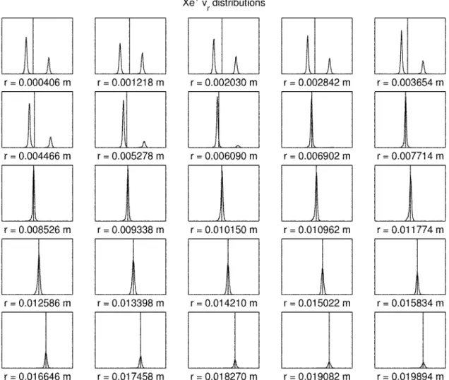
Instead of reading averaged information off of grid points, HPHall is modified to record data about particles crossing the exit plane at z = .030 m as seen in Figure 3-10. This plane is divided into 25 radial bins which in turn are sub-divided into axial and radial velocity bins. Single and double ion data are recorded separately so that distinct distributions for each species can be derived.
Since detailed information about axial and radial velocities is tracked, the new source model does not assume a constant ion drift velocity across the exit plane. Instead, functions for both velocity components, depending on radial position, are extracted from the HPHaII simulation data. This approach also eliminates the need for a beam divergence angle function as the direction of the particle is contained in the two velocities.
Figures 3-11 and 3-12 show the axial and radial velocity distributions of single ions at each radial bin. The vertical line in each plot marks the average velocity for that radius. Two distinct peaks are observed in the radial velocity distributions close to the thruster centerline. This phenomenon is attributed to the fact that as particles in
r = 0.000406 m r = 0.004466 m r = 0.008526 m r = 0.012586 m r = 0.016646 m r = 0.001218 m r = 0.005278 m r = 0.009338 m r = 0.013398 m r = 0.017458 m Xe* v distributions r = 0.002030 m r = 0.006090 m r = 0.010150 m r = 0.014210 m r = 0.018270 m r = 0.002842 m r = 0.006902 m r = 0.010962 m r = 0.015022 m r = 0.019082 m r = 0.003654 m r = 0.007714 m r = 0.011774 m r = 0.015834 m r = 0.019894 m
Figure 3-11: Xenon single ion axial velocity distributions. Horizontal axes are axial velocit, v2, ranging from 0 to 35000 m/s. Vertical axes are number of Xe+ ranging from 0 to 3 x 10¹².
HPHall cross the centerline grid boundary, they are reflected by reversing the sign of
their radial velocity in order to represent particles that are coming from the opposite side of the annular engine. It is clear that the calculated average velocity values for the radial component do not accurately reflect these two distinct populations of ions. Thus., HPHall is also modified to label particles reflected at the centerline differently from particles originating in the main engine channel so that the two populations can be investigated independently.
r = 0.000406 m r = 0.004466 m r = 0.008526 m r = 0.012586 m r = 0.016646 m r = 0.001218 m r = 0.005278 m r = 0.009338 m r = 0.013398 m r = 0.017458 m Xe+ v distributions r = 0.002030 m r = 0.006090 m r = 0.010150 m r = 0.014210 m r = 0.018270 m r = 0.002842 m r = 0.006902 m r = 0.010962 m r = 0.015022 m r = 0.019082 m r =0.003654m r = 0.007714 m r = 0.011774 m r = 0.015834 m r = 0.019894 m
Figure 3-12: Xenon single ion radial velocity distributions. Horizontal axes are radial
velocity, V,, ranging from -35000 to 35000 m/s. Vertical axes are number of Xe+ ranging from
0 to 4 x
1012.12 10 8 6 4 2 0 x 1016 +++ + ++ +++ 0 0.005 0.01 0.015 0. r (m)
x 1 013 r x number density distribution
14 ... 12 ++ +++++ 10 +++ 8 6 4 2 0 0 0.005 0.01 0.015 0. r (m) 2.5 2 E + 1 X0 0.5 rn 2.51 C E z X 2 1.5 0.5 x 10²² 0 0.005 0.01 0.0 r (m) X 1018 Fit to number density
0 0.005 0.01
r (m) Figure 3-13: Derivation of Xe+ number density distribution.
Single Ions
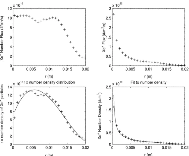
The same process described for the preliminary source model is used to generate the radial cumulative distribution function, except during conversion of the flux distri-bution to a number density distridistri-bution. Instead of dividing by an assumed ion drift velocity across the entire exit plane, flux at each radial position is divided by its corresponding average velocity. Figure 3-13 shows the procedure to obtain the radial cumulative distribution function given by,
Pe,+
=74.5992r
-
1244.3r
2+ 6.4753 x 10⁴r
3-
3.1991 x 10⁶,r
4.
(3.11)
As before, this CDF can be used to determine the radial position of a source ion.
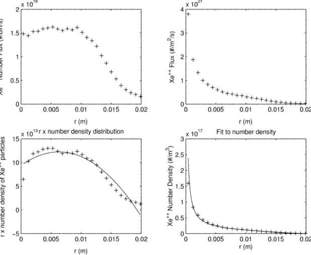
-S+ + S++ 15 0.02 0.015 0.02
.
L
02 02x 101 ~ -0 .0 E z3 0 0.005 0.01' r (m) * Total + Near-side population x Far-side population 5*** ***** 4 + 3 + + + * + * 2- x 2xx lxXX ** 01 x X 0 0.005 0.01 0.015 0.0 r(m) 5 4- + + 3j + + 2-(1 -+ 0.015 0.02 0 2 4 r (m)
Figure 3-14: Split of single ion populations.
However, for values below r = 0.007714 in, the ion may either be part of the
afore-mentioned near-side or side populations. The reason for this sharp cutoff in
far-side ions will be seen later. Figure 3-14 shows the split of the two ion populations and the fraction of ions coming from across the centerline as a function of radius. The first 10 radial bins, excluding the first data point, are used to find a fit for this fraction which is given by,
ffar-sideXe+ = = -1.2789
x
103r2 -58.7267r
+
0.5055.
rlnear-sideXe-+ + f'far-sideXe+
(3.12)
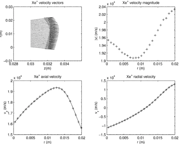
Each population of ions has its own axial and radial velocity functions. Figure 3-15 depicts the velocity distributions for the near-side population where the axial andFit to first 10 bins
0. U) ,0. E 2 0 0 .00. LL --+ 6 x 10-,0.8 E 0 '0.6 0 0.4
8
0.2 C.)Xet velocity vectors )28 0.03 0.032 0.034 z(m) x 10, Xet axial velocity 0.005 0.01 r (m) 0.015 0.02
x 104 Xet velocity magnitude 2.04r 2.02 0.03 0.02 + ++ ± + + + ++ + + + + 0.005 0.01 0. 0.005 0.01 0. r (m)
X 104 Xet radial velocity
2 131.98 1.96 1.94 1.92 1.9 1.5 0.5 E 0 -0.5 -1 -1.5 0
Figure 3-15: Single
ionnear-side population velocity distributions.
radial velocity functions are given by,
2.4597 x 101r6 - 1.2956 x 10¹⁴r- + 2.4102 x 10²r" - 2.0171 x 101013