A comparative study of DCT, LOT, and DWT-based image coders

A Comparative Study of DCT, LOT, and

DWT-based Image Coders

by

Warit Wichakool

Submitted to the Department of Electrical Engineering and Computer

Science

in partial fulfillment of the requirements for the degrees of

Bachelor of Science in Electircal Engineering and Computer Science

and

Master of Engineering in Electrical Engineering and Computer Science

at the

MASSACHUSETTS INSTITUTE OF TECHNOLOGY

June 2001

©

Warit Wichakool, MMI. All rights reserved.

The author hereby grants to MIT permission to reproduce and

BARKE

distribute publicly paper and electronic copies of this thesis document

in whole or in part.

OF TECHNOLOGY

JUL 11 2001

Author ... LIBRARIES

Department of Electrical Engineering and Computer Science

May 23, 2001

Certified by...

K.S. Thyagarajan

Principal Engineer

VIA

daiesisispupervisf

Certified by...

David H.itaelin

_-Professor of Electrical Engineering

WL.T ThesiS~uj rvisor

Accepted by...

Arthur C. Smith

Chairman, Department Committee on Graduate Students

A Comparative Study of DCT, LOT, and DWT-based Image

Coders

by

Warit Wichakool

Submitted to the Department of Electrical Engineering and Computer Science on May 23, 2001, in partial fulfillment of the

requirements for the degrees of

Bachelor of Science in Electrical Engineering and Computer Science and

Master of Engineering in Electrical Engineering and Computer Science

Abstract

Ten transform coding systems were compared in terms of their system complexity and peak signal-to-noise ratios (PSNR). The results showed that the relationship between PSNR and bit rate was affected by the combination of the quantizer and the encoder, but was not affected by the type of transform. The performance of the embedded zerotree wavelet (EZW) system was effected by the number of discrete wavelet transform (DWT) levels. In comparison with the 2-level EZW system at a given bit rate, the EZW system improved PSNR by up to 4 dB at low bit rates as the number of levels increased from two to three, and gained another 1 dB as the number of levels increased from three to four. Four of the ten systems were studied further: the discrete cosine transform (DCT) baseline JPEG, the lapped orthogonal transform (LOT) version of baseline JPEG, the visual threshold wavelet with the run-length Huffman coder, and the EZW with the adaptive Huffman coder. The PSNR values for the Lena image at 0.5 bit/pixel for the four systems were 34.56, 34.43, 34.97, and 34.52 dB, respectively. In comparison with the DCT JPEG, the LOT JPEG provided 0.5 dB better PSNR and also reduced the image blockiness, but it introduced small ringing artifacts in areas with sharp edges. The visual threshold wavelet yielded better PSNR than the DCT system at the same bit rate, but the reconstructed image suffered from blurriness. Finally, the EZW system performed comparably to the DCT system. Although the reconstructed image exhibited no blockiness, it clearly lost some details.

VI-A Company Thesis Supervisor: K.S. Thyagarajan Title: Principal Engineer

M.I.T. Thesis Supervisor: David H. Staelin Title: Professor of Electrical Engineering

Acknowledgments

I would like to take this opportunity to express my gratitude toward many people

on the course of my thesis. First of all, I would like to thank K.S. Thyagarajan for his advice and guidance. I also would like to thank Professor Staelin for his guidance and comments on my thesis, and Henrique Malvar for providing the programs and references of the LOT system for my simulation. I also would like to thank all members of Digital Cinema at QUALCOMM INCORPORATED for their supports during my research at the company. In addition, I would like to thank Peter Agboh and Songpon Deechongkit for their comments on my research. In addition, I have to thank Yui (Siraprapha Sanchatjate), my family, and all my friends for all the mental support and encouragement they have been giving me through out the years at MIT.

Contents

1 Introduction 2 Background

2.1 Transform . . . . 2.1.1 Discrete Cosine Transform . . . . 2.1.2 Lapped Orthogonal Transform . . . . .

2.1.3 Discrete Wavelet Transform . . . .

2.2 Quantization . . . .

2.2.1 Optimal Uniform Quantizer . . . . 2.2.2 JPEG Uniform Quantizer . . . .

2.2.3 Visual Threshold Wavelet Quantizer

2.2.4 Embedded Zerotree Wavelet Quantizer

2.3 Entropy Coding . . . .

2.3.1 Huffman Coding . . . .

2.3.2 Adaptive Huffman Coding . . . .

2.3.3 Run-Length Huffman Coding . . . . .

3 Simulation Methods

3.1 Part I: System Complexity . . . .

3.2 Part II: System Performance...

3.2.1 Part II-A: Effect of Number of

3.2.2 Part II-B: Effect of Transform

3.2.3 Part II-C: Effect of Quantizer

Levels on DWT Systems . . . . . 12 16 17 18 20 26 31 33 34 35 37 40 41 41 41 44 46 46 47 47 48

3.2.4 Part II-D: Effect of Entropy Coder . . . . 49

3.2.5 Part II-E: Overall System Performance . . . . 49

3.3 Part III: Visual Quality . . . . 50

3.4 Test Im ages . . . . 50

4 Results and Discussions 52 4.1 Part I: System Complexity . . . . 52

4.1.1 Transform . . . . 52

4.1.2 Quantization . . . . 54

4.1.3 Entropy Coding . . . . 55

4.2 Part II: System Performance . . . . 56

4.2.1 Part II-A: Effect of Number Levels on DWT Systems . . . . . 56

4.2.2 Part II-B: Effect of Transform . . . . 65

4.2.3 Part II-C: Effect of Quantizer . . . . 70

4.2.4 Part II-D: Effect of Entropy Coder . . . . 71

4.2.5 Part II-E: Overall System Performance . . . . 78

4.3 Part III: Visual Quality. . . . . 90

5 Summary 105

List of Figures

Basic transform coding system . . . . Block diagram for a separable 2-D transform Flowgraph conventions . . . .

1-D DCT basis functions . . . .

Fast DCT for M=8 ... Fast IDCT for M=8 ...

General structure of the LOT . . . . LOT basis functions ...

Type-I, fast LOT for a block size of 16 . . . .

Type-I, fast ILOT for a block size of 16 .... Type-I, fast LOT for the finite length signal .

2-level, 2-band analysis and synthesis for the 1-D DV Organization of 3-level DWT coefficients . . . . Locations of parent-descendants of the 3-level EZW Zig-zag scan of the run-length Huffman coder . . . . . Flowgraph of the run-length Huffman coder . . . .

4-1 Effect of number of DWT levels on the PSNR performance of the DWT systems using the EZW quantizer and the adaptive H uffm an coder . . . . 4-2 Efficiency test for the adaptive Huffman coder . . . . 4-3 bfragl: original image at 8 bpp . . . . 4-4 bfrag2: DCT + JPEG + Run-Length Huffman at 0.50 bpp .

. . . . 16 . . . . 18 . . . . 18 . . . . 19 . . . . 2 1 . . . . 22 . . . . 23 . . . . 25 . . . . 26 . . . . 27 . . . . 28 T . . . 30 . . . . . 31 . . . . . 39 . . . . . 43 . . . . . 43 64 89 93 94

4-5 bfrag3: 3-level DWT + EZW + Adaptive Huffman at 0.50 bpp 95 4-6 bfrag4: 4-level DWT + EZW + Adaptive Huffman at 0.50 bpp 96

4-7 bfrag5: 3-level DWT

+

Huff-man at 0.50 bpp ... ... 97

4-8 bfrag6: LOT

+

4-9 lenal: original image at 8 bpp ... . 99

4-10 lena2: DCT + JPEG + Run-Length Huffman at 0.50 bpp . . 100

4-11 lena3: 3-level DWT + EZW + Adaptive Huffman at 0.50 bpp 101 4-12 lena4: 4-level DWT

+

4-13 lena5: LOT + JPEG + Run-Length Huffman at 0.50 bpp . . 103

4-14 lena6: 3-level DWT + Visual Threshold + Run-Length

List of Tables

2.1 Computational costs of the fast DCT . . . . 21

2.2 Computational costs of the type-I, fast LOT . . . . 29

2.3 Coefficients of 9/7-tap Villasenor biorthogonal filters . . . . . 29

2.4 Computational costs of the DWT . . . . 32

2.5 Basis function amplitudes for 9/7-tap biorthogonal filters . . 36

2.6 Quantization levels for 9/7-tap biorthogonal filters . . . . 37

3.1 List of tested transform coding systems . . . . 44

3.2 List of systems for comparing the effect of number of DWT levels on the PSNR performance . . . . 47

3.3 List of systems for comparing the effect of transforms on the PSNR performance using the optimal uniform quantizer, the Huffman coder, and the run-length Huffman coder . . . . 48

3.4 List of systems for comparing the effect of quantizers on the PSNR performance using the run-length Huffman coder . . . 49

3.5 List of systems for comparing the effect of entropy coders on the PSNR performance using Huffman and run-length Huff-m an coders . . . . 49

3.6 List of selected systems for comparing the PSNR performance 50 3.7 List of test im ages . . . . 51

4.1 Computational costs of transform algorithms . . . . 53

4.3 List of systems for comparing the effect of DWT levels on the PSNR performance of the DWT systems . . . . 57

4.4 Effect of DWT levels on the PSNR performance of the DWT

systems using the optimal uniform quantizer and the

run-length Huffman coder ... 58

4.5 Effect of DWT levels on the PSNR performance of the DWT

systems using the optimal uniform quantizer and the

run-length Huffman coder (cont.) ... 59

4.6 Effect of DWT levels on the PSNR performance of the DWT

systems using the visual threshold quantizer and the

run-length Huffman coder ... 60

4.7 Effect of DWT levels on the PSNR performance of the DWT

systems using the visual threshold quantizer and the

run-length Huffman coder (cont.) ... 61

4.8 Effect of DWT levels on the PSNR performance of the DWT

systems using the EZW quantizer and the adaptive Huffman co d er . . . . 62

4.9 Effect of DWT levels on the PSNR performance of the DWT systems using the EZW quantizer and the adaptive Huffman coder (cont.) . . . . 63

4.10 List of systems for comparing the effect of transforms on the

PSNR performance ... 65

4.11 Effect of transforms on the PSNR performance using the

op-timal uniform quantizer and the Huffman coder ... 66

4.12 Effect of transforms on the PSNR performance using the

op-timal uniform quantizer and the Huffman coder (cont.) . .. 67

4.13 Effect of transforms on the PSNR performance using the op-timal uniform quantizer and the run-length Huffman coder . 68

4.14 Effect of transforms on the PSNR performance using the op-timal uniform quantizer and the run-length Huffman coder

(con t.) . . . . 69 4.15 List of systems for comparing the effect of quantizers on the

PSNR performance using the run-length Huffman coder . . . 71 4.16 Effect of quantizers on the PSNR performance of the DCT

systems using the run-length Huffman coder . . . . 72 4.17 Effect of quantizers on the PSNR performance of the DCT

systems using the run-length Huffman coder (cont.) . . . . 73 4.18 Effect of quantizers on the PSNR performance of the LOT

systems using the run-length Huffman coder . . . . 74 4.19 Effect of quantizers on the PSNR performance of the LOT

systems using the run-length Huffman coder (cont.) . . . . 75 4.20 Effect of quantizers on the PSNR performance of the DWT

systems using the run-length Huffman coder . . . . 76 4.21 Effect of quantizers on the PSNR performance of the DWT

systems using the run-length Huffman coder (cont.) . . . . 77 4.22 List of systems for comparing the effect of entropy coders on

the PSNR performance using the optimal uniform quantizer 78

4.23 Effect of entropy coders on the PSNR performance of the

DCT systems using the optimal uniform quantizer . . . . 79

4.24 Effect of entropy coders on the PSNR performance of the

DCT systems using the optimal uniform quantizer (cont.) . . 80

4.25 Effect of entropy coders on the PSNR performance of the LOT systems using the optimal uniform quantizer . . . . 81

4.26 Effect of entropy coders on the PSNR performance of the

LOT systems using the optimal uniform quantizer (cont.) . . 82

4.27 Effect of entropy coders on the PSNR performance of the DWT systems using the optimal uniform quantizer . . . . 83

4.28 Effect of entropy coders on the PSNR performance of the

DWT systems using the optimal uniform quantizer (cont.) . 84

4.29 List of selected systems for the comparison in PSNR perfor-m an ce . . . . 85

4.30 Comparison of the PSNR performance of DCT, LOT, and

DWT systems ... ... 86

4.31 Comparison of the PSNR performance of DCT, LOT, and

DW T systems (cont.) ... . 87

Chapter 1

Introduction

Modern media is overwhelming with graphics such as images and movies. Constraints on bandwidth and memory space create trade-offs between the size and quality of images. One solution is to compress the image using a transform coding system. The basic transform coding system consists of three blocks: a transform block, a quantization block, and an entropy coding block. At a given bit rate, different systems yield different image quality. In addition, each system varies in terms of the algorithm complexity. Within the system, the complexity and the image quality may be mainly influenced by a single functional block or by a combination of all three blocks. It is hard to determine the best system to use.

One of the most popular compression systems uses the discrete cosine transform

(DCT) system recommended by Joint Photographic Experts Group (JPEG). The

simplest JPEG system is the baseline JPEG. This system combines the DCT with a uniform scalar quantizer and a run-length Huffman coder [1], [9]. The DCT system provides high quality images at reasonable bit rates, but exhibits blockiness at low bit rates. This artifact is caused by independent processes of transformed blocks and the discontinuity of the DCT basis functions [7], [14]. This artifact can be reduced by increasing the bit rate or using more complex systems. However, the gain in quality may not justify additional complexity of the system.

Another solution to reduce the blocking effect is to change the transform block to the lapped orthogonal transform (LOT). This transform solves the problem by

overlapping and modifying the DCT basis functions to eliminate the independent transformation of image blocks and the discontinuity of the basis functions [7]. The LOT is similar to the DCT because it is a block transform. Furthermore, the LOT uses the DCT bases as its building blocks for new basis functions [7]. However, there is no standard quantizer and entropy coder for the LOT system. Since the LOT is similar to the DCT, the LOT may benefit from the JPEG-like quantizer and encoder in the same way as the DCT. Therefore, the reduction of the blocking effect can be done by modifying the transform block to the LOT and updating parameters for the quantizer and the encoder accordingly. This solution may be the simplest one to improve the visual quality of the image.

Recently, the wavelet-based system has been extensively studied and developed for image compression applications. Many of the candidates for the JPEG-2000 standard are wavelet-based [6]. The discrete wavelet transform (DWT) is one of sub-band coding. One implementation of DWT system employs a filter bank to separate the signal into a number of frequency bands. Each band is then quantized and encoded depending on the systems. These filter banks operate on the whole image instead of a block like the DCT and the LOT. As a result, it should eliminate the image blockiness completely. In addition, the DWT system can gain compression from a special structure called a zerotree. Sample encoders based on this structure are the embedded zerotree wavelet (EZW) and the set partitioning in hierarchical trees (SPIHT). Both encoders use a bit-plane coding scheme and the zerotree structure to compress the information and are claimed to provided higher PSNR than the baseline

DCT JPEG at given bit rates [10], [11]. In addition, both the EZW and the SPIHT

are embedded systems that can achieve the targeted bit rate exactly. Furthermore, the encoders do not have to send a code table in the encoded file because the decoders will generate the code table during the decoding process [11]. These properties allow both systems to perform progressive coding. Another wavelet system is the visual threshold system. It uses a predefined quantization level for each wavelet band [16]. This quantization scheme is similar to the baseline JPEG. Therefore, this system can be adapted to use the run-length coder of the baseline JPEG system with some

modifications.

The choices above present alternatives for image compression. All transform cod-ing systems may achieve the same PSNR and bit rate but at different costs. Since the system consists of three functional blocks: the transform, quantizer, and entropy coder, the performance of each system may depend on one particular block or the combination of the blocks. It is useful to compare the PSNR gain for each type of transform, quantizer, and entropy coder independently. The PSNR gain of the transform block can be compared by using the same type of the quantizer and the entropy coder for all transforms. The PSNR gain, as a result, is influenced mainly

by the transform block. The comparison of quantizers can be done by restricting the

choice of transform and entropy coder to be the same for all compared systems. The comparison of entropy coders can be done in a similar manner. The results of these comparisons should reveal the optimal encoding scheme for each transform.

This thesis compared several transform coding systems in terms of their system complexity and peak signal-to-noise ratios (PSNR) at given bit rates. The tested transforms included the discrete cosine transform (DCT), the lapped orthogonal transform (LOT), and the discrete wavelet transform (DWT). The tested quantiz-ers included the optimal uniform quantizer, the JPEG uniform quantizer, the visual threshold quantizer, and the embedded zerotree wavelet (EZW). Finally, the tested entropy coders included the Huffman coder, the adaptive Huffman coder, and the run-length Huffman coder. The system complexity was compared in terms of number of additions and multiplications. This thesis focused primarily on the transform block for the complexity comparison. However, comparisons of quantizers and entropy coders were also included. Selected combinations of these three components were used to study the influence of each component on the PSNR performance. Finally, four systems were studied further to compare overall system performance including the visual quality of reconstructed images. They were the baseline DCT JPEG, the baseline LOT JPEG, the visual threshold wavelet with the run-length Huffman coder, and the EZW with the adaptive Huffman coder. In all comparisons, seven standard test images were used, including Lena and Barbara.

This thesis is organized as follows. Chapter 2 presents background and algorithm implementation of the functional blocks used in this thesis. Chapter 3 presents lists of comparison methods and corresponding tested systems. In Chapter 4, the results are presented and discussed, Finally, the thesis is concluded and further studies are proposed in Chapter 5.

Chapter 2

Background

This chapter presents brief background and algorithm implementation of all compo-nents of the still image compression used in this thesis. A simple transform coding system consists of three fucntional blocks: transform, quantization, and entropy cod-ing. A block diagram of a simple encoder/decoder system is shown in Figure 2-1 below.

original Entropy compressed S Transform Quantization Cdn mg

image Coding image

(a)

reconstructed Inversed Entropy compressed image Transfom Dequantization Decoding image

(b)

Figure 2-1: Block diagram of a basic transform coding system for still image copmression (a) The encoding part of the system. (b) The decoding coun-terpart of the system

An original image is passed through the transform block that outputs transform coefficients. The quantizer then reduces the coefficients to fewer numbers or symbols.

Finally, the entropy coder translates those numbers or symbols into a stream of binary bits in order to be stored or transmitted. In this thesis, lists of all components in the simulation are shown as follows.

" Transform:

(a) Discrete Cosine Transform (DCT)

(b) Lapped Orthogonal Transform (LOT)

(c) Discrete Wavelet Transform (DWT)

" Quantization:

(a) Optimal Uniform Quantizer

(b) JPEG Uniform Quantizer

(c) Visual Threshold Wavelet Quantizer

(d) Embedded Zerotree Wavelet Quantizer (EZW)

* Entropy Coding:

(a) Huffman

(b) Adaptive Huffman

(c) Run-Length Huffman

The quantizers and coders listed above may be specifically designed for particular transform coefficients. Some modifications are required in order to use the same quantizer or entropy coder for different transforms. The modifications are described in the background section of that particular algorithm.

2.1

Transform

The transform block is used to remove redundancy of the information of the input signal, an image in this case [1], [4], [8]. The image signal is projected onto a partic-ular set of basis functions. In general, the basis functions are orthonormal in order

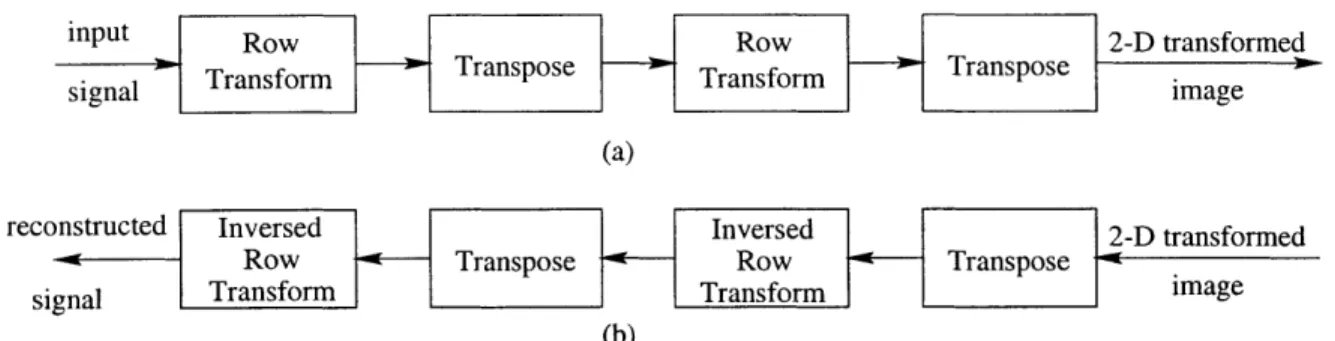
to minimize the redundancy in the representations. In this thesis, all transforms are either orthogonal or nearly orthogonal because of the advantages of fast algorithms. Furthermore, all transforms are separable, meaning the transform can be performed on each dimension independently. This property reduces the complexity of the im-plementation significantly. The separable 2-D transform can be computed according to the diagram shown in Figure 2-2 below. There are three transforms used in this thesis: the DCT, the LOT, and the DWT. The details of each transform are discussed in the sections below. In addition, there are some conventions of the flowgraphs used in this thesis. All conventions are shown in Figure 2-3 below.

input Row Row 2-D transformed

- Transform Transpose Transform Transpose image

(a)

reconstructed Inversed Inversed 2-D transformed Row Transpose Row Transpose : a

signal Transform Transform image

(b)

Figure 2-2: Block diagram for a separable 2-D transform

a a+b a a-b a c c*a

b b

Figure 2-3: Flowgraph conventions

2.1.1 Discrete Cosine Transform

The discrete cosine transform (DCT) is an orthogonal block transform. It projects each block of the input signal onto a set of truncated, sampled cosine waveform. The computation of the DCT coefficients can be done as follows. Let M be the block length, k be the index of the basis function, and n be the sample index, the basis

functions of the 1-D DCT are given by = ] Cos (nk+ ) k 2 2 M ; O<k<M-1, r- ; k=O 2 1 ; otherwise.

First four basis functions of the 1-D DCT are shown in Figure 2-4 below.

(a) ) 2 4 6 E (c)

-T-'1111.'

T

Figure 2-4: First four basis functions of the 1-D DCT for M=8

The 2-D DCT is a separable transform. The 2-D transform can be done as

previ-ank where (2.1) c[k] (2.2)

0

ously shown in Figure 2-2 above. In the case of one dimensional transform, the DCT coefficients, X[k], can be calculated as follows. Let x[n] be an input signal indexed

by n and M is the DCT block length, X[k] is given by

2 M-1 Ik X[k] = c[k] [n] Cos (n + 2) 0 k < M-1, (2.3) n:=O where -k0 c[k] =- v' 1 ; otherwise.

The inverse discrete cosine transform (IDCT) is given by

V2 2 M1 [1k 7r] 0 O<ni< M -l, (24

z~~n] = ~~c[k]ZC[k] _{cos (n + 2) ; _<M-, (24}

Mk= O[ M (2.4

where i[n] is a reconstructed signal and k[k] is the dequantized DCT coefficient. All other symbols are the same as those in the DCT algorithm shown above. In this thesis, the transform block has a length of 8 for 1-D transform and a size of 8x8 for

2-D signal. The fast algorithms for DCT and IDCT are shown below in Figure 2-5

and 2-6 respectively. The DCT algorithms can be found in [6].

Finally, the computational costs of the 1-D and 2-D DCT algorithms used in this thesis are summarized in Table 2.1 below. The costs of the IDCT algorithms are the same as the DCT. The computational costs shown below assumes that the image dimension is RxC, where R is the number of rows and C is the number of columns. In addition, it is assumed that R and C are divisible by 8 in this thesis.

2.1.2

Lapped Orthogonal Transform

Although the DCT has been employed extensively in still image compression, the DCT system exhibits blocking artifact at low bit rates. The lapped orthogonal transform (LOT) was developed to minimize this artifact. The causes of the blocking

1/(2sqrt(2)) x[O] m[0 n[O] n[0 X[0] 1/(2sqrt(2)) x[1] m[1 n[1] n[1- --- X[4] x[2] m[2 - -- - n[2] n[2] (C2)/2 X[2] (S2 (S2)/2 x[3] m[13 --- n[3] n[3 --- - X[6] x[4] - - m[4 m[4] n[4] p[4 (Cl)/2 X[1] (S1)/2 (S1)/2 x[5] - - m[5 m[5] n[5] p[5 --- X[7] 1/sqrt(2) (C 1)/2 x[6] ---- m[6 m[6 n[6]1 n[6 --- p[6 (C5)/2 X[5] 1/sqrt(2) (S5)/2 (S5)/2 x[7]--- m[7 m[7 - n[7] n[7 --- _p[7 - (C5)/2 X[3]

Figure 2-5: Flowgraph of Fast DCT for M=8 Ci represents cos(

)

Si represents sin( ).

Table 2.1: Computational costs of the fast DCT, M=8

effect can be divided into two categories. First, the DCT bases are short, non-overlapped, and discontinuous at the edges. Second, the DCT system transforms each block independently. The LOT eliminates this artifact by forcing the bases to decay to zero at both edges and overlapping with a neighboring transform block [7], [14]. In this thesis, the overlapped part was half of the block length and started at the middle of the preceding block. The general structure of LOT is shown in Figure

2-7.

In order to make the LOT an orthogonal transform, all the bases must form an orthonormal set. Furthermore, the overlapped portion must be orthogonal to all bases

#

#

1-D, 8-point DCT 26 16

RxC, 2-D DCT 13RC 4RC

1/(2sqrt(2)) X[O] n[] n0n[] m[O] 1/(2sqrt(2)) X[4] - - - n[1] n[1] m[1] (C2)/2 X[2] n[2 n[2] m[2] (S2)>: (/2 X[6] -- - n[3 n[3] --- -m[3] X[1] p[4] n[4] (C1)/2 m[4] (S1)/2 (S1)/2 X[7] p[5 n[5 --- _{(C 1)/2} -m[5] X[3] p[6] 1/sqrt(2) p[6 --- --- n[6] (C5)/2 m[6] /sqrt(2) 5)/2 X[5] -p[7] p[7 ---- -- n[7 -- (C - - m[7] m[O] m[1] m[2] m[3] m[4] -m[5] --m[6] -m[7] -N'r

Figure 2-6: Flowgraph of Fast IDCT for M=8 Ci represents cos( ) and

Si represents sin( ).

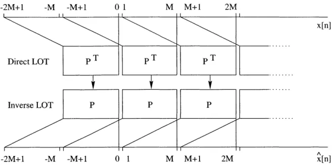
of the neighboring block [5]. It is not practical to use the original version of the LOT because there was no fast algorithm available. However, the nearly orthogonal lapped transform has a fast algorithm. This type of LOT, called the type-I, fast LOT, uses bases of DCT as building blocks for its bases. This algorithm requires few additional computations beyond the existing DCT algorithm [7].

The LOT coefficients can be calculated as follows. Let M be the length of a transform block, V is the overlapped length, where M - 2V. The transform pair is given by

X = PTX (2.5)

and

x = PX, (2.6)

where P is the basis function matrix whose size is MxV. x is an input vector of

x[0] x[1] x[2] x[3] x[4] x[5] x[6] x[7]

-2M+1 01 M M+l 2M

p T

Figure 2-7: General structure of the LOT In this structure, the overlapped portion is a half of the block length. PT and P are the transform and the inverse transform operator respectively.

length M. The basis function matrix, P, for the fast algorithm is given by

P = P0Z, (2.7)

where P is the MxV matrix and Z is the orthogonal matrix of size VxV. The matrix

Po is given by

De Do J(De - Do)

De - Do

-J(De - Do)

De and Do are the even and odd functions of the DCT bases. J is an anti-identity matrix. Z is approximated in the fast algorithm as

I 0 , 7 0 Z (2.9) 1 PO= (2.8) -2M+1 0 1 2M Z ~ M M+1

where

Z

Z

Z

where matrix T is an m by ! matrix. It is defined as

1 0 0

Ti= 0 Y(0j) 0 . (2.11)

0 0 I

Y(Oj) is a rotational matrix in the position (i, i) of the matrix T. Y is a 2x2 matrix and is defined as

Y(00 cos Oi sin Oi (2.12)

- sin Oi cos O6

where Oi is a rotation angle.

In this thesis, the type-I, fast LOT had the block length, M, of 16 and the over-lapped length, V, of 8 because the 8-point fast DCT can be used as part of LOT algorithms. The matrix

Z

are [0, 01, 02] = [0.137r, 0.167r, 0.137r] for the optimal coding gain, and [00, 0

1, 02]

= [0.1457r, 0.177r, 0.167r] for the QR-based quasi-optimal LOT [5]. This thesis used

the angle for the optimal coding gain. The first four basis functions of the type-I, fast LOT for optimal coding gain with the block length of 16 samples and overlapped portion of 8 samples are shown in Figure 2-8 below. The implementations of type-I, fast LOT block transform and inverse transform are shown in Figure 2-9 and 2-10 respectively. The LOT programs can be found in [6]. In addition, all figures of the LOT system were reproduced with the permission of Henrique Malvar.

In the case of a finite length signal, the beginning block and the ending block must be modified to support the non-existing overlapping part. It is done by reflecting few samples of the beginning and the ending block outside the signal. Then the reflected parts are treated as part of the signal. In this thesis, only first and last four samples

1 0.5 0 -0.5 0 Figure V = 8 5 10 1 0.5 0 -0.5 (a) 0(D 0 5 10 1 (c)

OT

T

-T

iI

T

ii

jj

0

TI

jj

2-8: First four basis functions of the type-I fast LOT, for M = 2V,

were reflected in order to compute the 8-point DCT of the first and the last block. As a result, only the even DCT coefficients are non-zero and the algorithm uses only the non-zero coefficients to compute the LOT coefficients. The type-I, fast LOT of a finite length signal is shown in Figure 2-11.

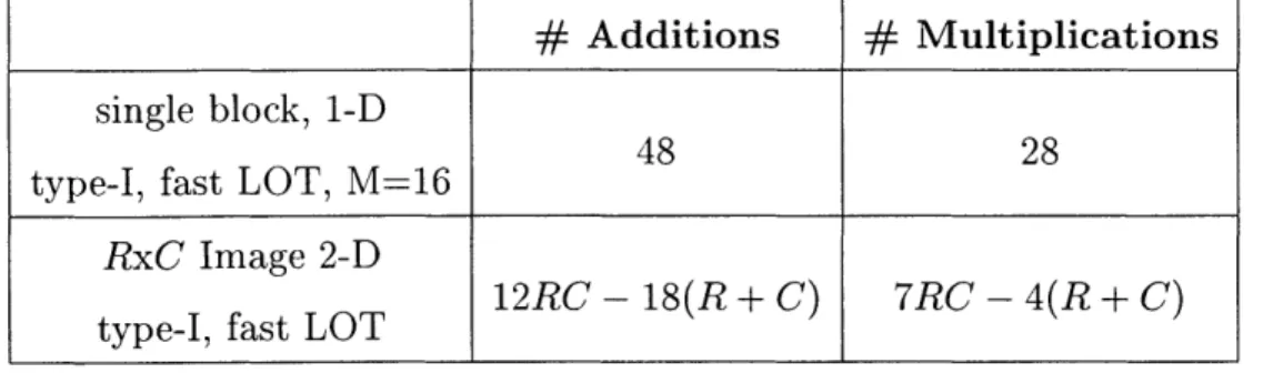
The computational costs for the type-I, fast LOT are summarized in Table 2.2, where R and C are image dimension. In this thesis, both R and C are assumed to be divisible by 8. The computational costs for the whole image take into account the half length DCT of all edges of the transformed image.

-1 -1 1 0.5 0 -0.5 -1 5 15

br x [0] 0-4 r b x [1] -r b x [2] w---r b x [3] Sb x [4] b x r[5] b x [6] b r b x [7] -r b X _{[+ 0] 0} xr+1t] * b x r+12] -b r+1 b xr+ _14] b r+151 _* b "r+ 11 _b "r+ 17 0 0

Figure 2-9: Flowgraph of the type-I fast LOT, for M = 2V, V = 8

2.1.3

Discrete Wavelet Transform

The discrete wavelet transform (DWT) uses the wavelet expansion to represent the signal in different time scales or spatial resolutions. The DWT is a series expansion of a finite length signal. The expansion consists of an approximation and a wavelet or detail. The wavelet expansion can be implemented by a filter bank. The derivation and detailed explanation can be found in [2], [13], and [12]. The filter bank algorithms have been well known for a long time. Therefore, the development cost for the DWT algorithm using the filter bank is practically low.

There are two stages for the DWT system. The transform process of the DWT is called an analysis stage. The inverse DWT is called a synthesis stage. The analysis stage separates the input signal into a set of octave-band frequency bands, whereas

1 2 2 4 3 6

DCT

DCT

X[0] X[2] X[4] X[6] -- ---- - -a X[1] - - -X[5] - -X[7]

---0i~

Figure 2-10: Flowgraph of the type-I fast ILOT, for M = 2V, V = 8

can be calculated as follows. The input signal, x[n], is passed through two filters: a low-pass filter and a high-pass filter. Ideally, the cut-off frequency of both filters should be at . Then the output signal of both filters are decimated by a factor of two. To further divide the frequency band, the output of the fist stage can be passed through the same set of filters. However, the distribution of DCT coefficients of a normal image consists of mostly low frequency components. Therefore, only the output of the low-pass filter from the first stage is used as the input to the second

stage filter banks. At the second stage, the length of input signal is half of the original length. The process can be repeated many times as long as the length of the input signal is longer than or equal to the length of the longest filter. Furthermore, the computational costs of the DWT increase according to number of levels or stages that the image is passed through. During the synthesis, the synthesis filters undo

x r [0] x [1] Xr[2] Xr[3] x r [4] xr[5] x [6] r x [7] r X r+i[0] x [1 r+1 x [2] r+1 x [3] r+1 x [4] r+1 x [5] r+1 x [6] r+1 x [7] r+1

2 1/2 W He Block 1 0-E1/2

1E

Z

Figure 2-11: Flowgraph of the type-I, fast LOT for a finite length signal

The LOT runs from left to right without the factor 2 after He and JHe. The inverse LOT runs from right to left. E is a set of even DCT coefficients and 0 is a set of odd

DCT coefficients.

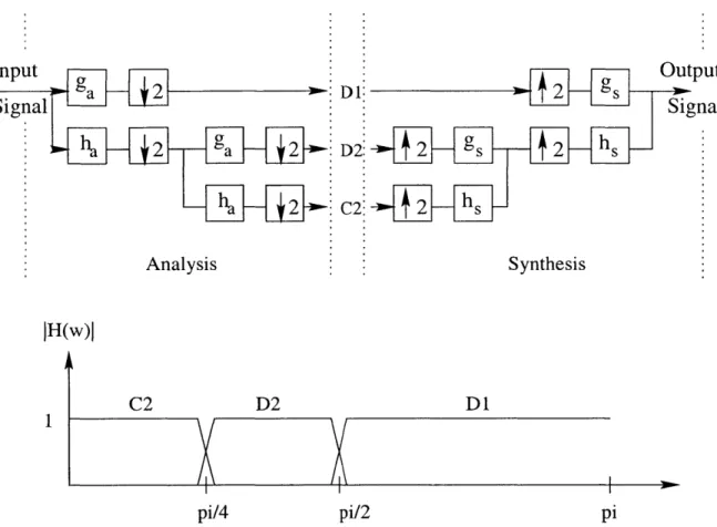
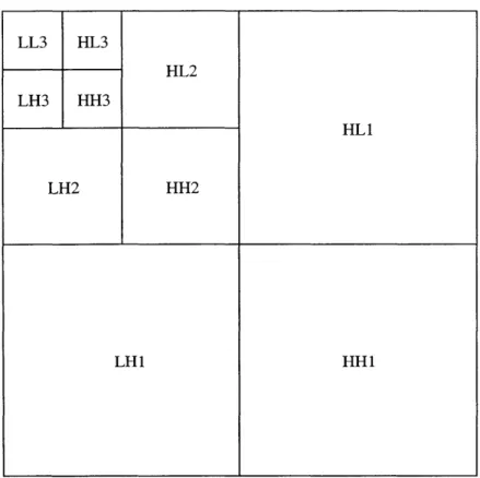
the analysis part by combining the highest level first, and then reconstructing the signal in the lower level. The structure of the 2-level analysis and synthesis DWT and the corresponding frequency bands are shown in Figure 2-12 below. In addition, the 2-D DWT is also separable. Therefore, the 2-D DWT can be calculated in each dimension independently, as previously shown in Figure 2-2 above. After the 2-D transformation of the image, the coefficients are organized in a certain way. An example of the organization of the 3-level DWT coefficients is shown in Figure 2-13 below.

The DWT coefficients also depend on the type of filter used. There are two kinds of filters: orthogonal and biorthogonal. The orthogonal filters are asymmetric and have

LOT of Block 1 LOT of Block 2 LOT of Block 3

Table 2.2: Computational costs of the type-I, fast LOT, M = 2V, V = 8

#

#

single block, 1-D

48 28

type-I, fast LOT, M=16 RxC Image 2-D

type-I, fast LOT 12RC - 18(R + C) 7RC - 4(R + C)

non-linear phase in the frequency response. The non-linear phase creates distortion or artifact in the reconstructed image, which is undesirable for image processing. On the other hand, the biorthogonal filters are symmetric and have linear or zero phase in the frequency domain. Therefore, it is desirable to use linear phase FIR filters for image processing. This thesis used 9/7-tap Villasenor biorthogonal filters [15]. The coefficients of both filters for the low-pass version are shown in Table 2.3 below.

Table 2.3: Coefficients of 9/7-tap Villasenor biorthogonal filters

The orthogonality in the biorthogonal system is preserved by the between the analysis filters and the synthesis filters. The relationships four filters are

ga[n] = (-1)"hs[1 - n] relationships among these (2.13) and g,[n] = (-1)nha[1 - n] Length Coefficients 0.03828, -0.023849, -0.110624, 0.377402, 0.852699, 9_ 0.377402, -0.110624, -0.023849, 0.03828 -0.064539, -0.040689, 0.418092, 0.788486, 0.418092, -0.040689, -0.064539 (2.14)

Output Signal D2S 2 s - e s C2: 2 _h Synthesis C2 D2 DI pi/2

Figure 2-12: Structure of 2-level, 2-band analysis and synthesis for the 1-D DWT and the frequency band to which the output of each filter bank

corresponds ga is a high-pass analysis filter. ha is a low-pass analysis filter. g8 is

a high-pass synthesis filter. h, is a low-pass synthesis filter.

where g, is a high-pass analysis filter, ha is a low-pass analysis filter, g, is a high-pass synthesis filter, and h, is a low-pass synthesis filter [2].

In this thesis, the DWT algorithm was derived from the WaveLab802 MATLAB package from Stanford university. The programs can be found in [3]. Parts of the pro-grams were translated into C propro-grams to reduce the simulation time. The MATLAB programs were used for verification purpose.

The computational costs for the algorithm are given in two types: the circular convolution algorithm and the minimum limit. The fist one is the circular convolution algorithm, which was used in this thesis. The second one is the minimum limit, which has lower computational costs by exploiting the symmetry of the biorthogonal filters.

Input a9- 2 Signal ha 2-- a 2 Analysis jH(w)l 1 pi/4 pi

Figure 2-13: Organization of 3-level DWT coefficients

The computations, especially multiplication, can be reduced significantly by reusing the the previous results. Given the filter length, F, only are distinct values

2

for the odd-length symmetric filters. Let the length of the filters be F and F2, where

F = F + F2, the computational costs for both cases are summarized in Table 2.4

below. These costs were calculated for the odd-length biorthogonal wavelet filters only. However, the cost of the even-length filters should be similar.

2.2

Quantization

The quantization block is used to limit the range of transform coefficients. This block gives the compression gain for the system. However, it introduces loss in the system. There are many quantization schemes used in the lossy image compression. This thesis used four quantizers, listed as follows.

LL3 HL3 HL2 LH3 HH3 HLI LH2 HH2 LHl HHi

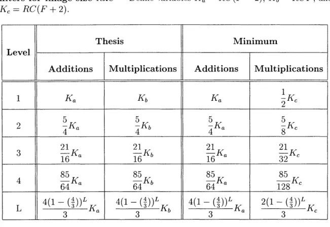
Table 2.4: The computational costs of L-level DWT using biorthogonal

filters for image size RxC Define variables Ka = RC(F - 2), Kb= RCF, and

Ke = RC(F + 2).

Thesis Minimum

Level

Additions Multiplications Additions Multiplications

1 1 Ka Kb Ka 2

Ke

(a) Optimal Uniform Quantizer

(b) JPEG Uniform Quantizer

(c) Visual Threshold Uniform Quantizer

(d) Embedded Zerotree Wavelet Quantizer (EZW)

The following sections explain algorithms, advantages, and disadvantages of the above quantizers. It should be noted that certain quantizer, such as the JPEG uniform quan-tizer, is specifically designed for the block-based DCT coefficients. Some modifications were made in order to adapt these quantizers to work with LOT coefficients. The modifications are explained in more detail in the section of that particular quantizer.

2.2.1

Optimal Uniform Quantizer

This quantizer is designed for a specific set of transform coefficients in order to minimize the mean square error (MSE). This quantizer is constructed from the statis-tics of the transform coefficients. Theoretically, it should give the smallest MSE which indicates the best performance according to the PSNR value used in this thesis. This quantizer was used in order to provide a fair comparison among all transform coding schemes because it is not optimally designed for any particular transform. In order to apply this quantizer to the coefficients of DCT, LOT, and DWT, there are three factors to be considered. First, how many quantizers are necessary. Second, which quantizer does each coefficient use. Finally, how to distribute the bit resources for each quantizer.

To answer these questions, let us look at the derivation and the organization of transform coefficients. The DCT and the LOT are block transforms whereas the DWT is not. The DCT and the LOT coefficients are arranged in a block of size 8

by 8 in this thesis. Each coefficient in this 8x8 block corresponds to different basis

functions in the 2-D transform. Furthermore, the coefficients that are located at the same location in the 8x8 block of different blocks correspond to the same basis function. Therefore, it is reasonable to use the same quantizer for each coefficient of the same basis function. As a result, there are 64 different quantizers for DCT and LOT transform coefficients because there are 64 distinct frequencies. In the case of the DWT, the coefficients are organized in the frequency bands. Similarly, wavelet coefficients in different bands use different quantizers. Given L-level DWT, there are

3L + 1 distinct quantizers.

The bit distribution problem can be solved by the rate-distortion theory as de-scribed in [1]. Given the average bit rate, B, the bit allocated to the ith quantizer,

bi, is

1 o.2

bi= B + 1og2 N, (2.15)

where ao is the variance of the coefficients in the ith group, and N is the total number of groups, i.e. 64 for the DCT and the LOT. Next, the width of each bin or the quantization level, qi, can be computed by

qi = k max,(IAi (2.16)

2bi

where max(IAil) is the maximum magnitude of the ith group, bi is the number of bits allocated for the ith group, and k is the scaling factor, which can be used to change the final bin width and adjust the bit rate. This scaling factor does not effect PSNR but enables the simulation to adjust the bit rate close to the desired value. Finally, the quantized coefficients, j, is calculated by dividing each input coefficient by the corresponding quantization level, i.e.

a

Ci qj

The advantage of using this quantizer is that the quantizer is symmetric around zero, also called flat-zero [1]. This property would benefit the system if the coefficients

have zero mean value because the distribution of the coefficients would be symmetrical about zero. There are encoders that can take advantage of this kind of distribution. Details of the coding schemes are presented in the next sections.

2.2.2

JPEG Uniform Quantizer

This quantizer is similar to the optimal uniform quantizer but it is specifically designed for block-based DCT coefficients. The JPEG standard recommends the quantization level for each frequency in the transformed block. These levels are derived from experimental results based on of many images and subjects in order to give the best visual quality for a given bit rate [1], [9]. This thesis used the following

quantization table for the black & white image. 16 11 10 16 24 40 51 61 12 12 14 19 26 58 60 55 14 13 16 24 40 57 59 56 14 17 22 29 51 87 80 62 Q = (2.18) 18 22 37 56 68 109 103 77 24 35 55 64 81 104 113 92 49 64 78 87 103 121 120 101 72 92 95 98 112 100 103 99

The top left hand corner corresponds to the quantization level for the DC compo-nent. The bottom right hand corner is the quantization level for the highest frequency component of the transform coefficients in 2-D. This table is the recommended quan-tization levels for the luminescence component according to the JPEG standard [9].

Although this quantizer is specifically designed for the DCT coefficients, the LOT coefficients might be able to use this quantization matrix because the LOT uses the

DCT as part of its building block for bases. Therefore, this thesis compared the

performance of the DCT system and the LOT system using this quantizer. The quantized coefficient, c3, is computed by a division operation as in equation (2.17).

2.2.3

Visual Threshold Wavelet Quantizer

This quantizer is intended to preserve the visual quality of the reconstructed image for the DWT coding system. The development of this quantizer was similar to those of the JPEG uniform quantizer. The quantization levels depend on the experimental results of the DWT coefficients. They also depend on the type of wavelet filter and number of levels of the DWT structure. In this thesis, only 9/7-tap biorthogonal filters were used. The DWT coefficients that belong to the same frequency band share the same quantizer. There are three bands at each DWT level with an exception of the coarsest level which has four bands. In other words, given the number of DWT levels,

L, there are 3L

+

QL,O,

{LL,

QL,O k 2 a1O [log (o

)J

AL,O (2.19)

where

" AL,O : the basis function amplitude

" a empirical value = 0.495

Sko: empirical value = 0.466

* fo empirical value = 0.401

e go : orientation parameter, JHL = 9LH = 1, 9LL 1.501, and gHH= 0.534

" r output resolution (pixel/degree) " L: number of DWT levels

* k scaling factor for adjusting quantization levels and bit rate

In the case of the 9/7-tap biorthogonal filters, values of AL,O and QL,O are shown in Table 2.5 and 2.6 respectively.

Table 2.5: The basis function amplitudes, AL,O, for 9/7-tap biorthogonal wavelet filters Orientation 1

1

Table 2.6: Quantization levels for 9/7-tap biorthogonal filters The output resolution is set at 32 pixel/degree.

Orientation

The quantized coefficient is computed by dividing the DWT coefficients with the corresponding quantization level. According to the quantization table given above, the coefficients in the higher frequency band are quantized more heavily than the low frequency coefficients. This property is similar to the quantization for the JPEG system. Models and development processes of this quantizer can be found in [16].

2.2.4 Embedded Zerotree Wavelet

Quantizer

The embedded zerotree wavelet (EZW) quantizer combines the bit-plane encoding and the zerotree structure to compress the data. The zerotree structure captures re-lationships among the magnitude of the DWT coefficients across different levels. The bit-plane part extracts each plane of bits, and the encoder searches for zerotree struc-tures and encodes them into symbols. The combination of the EZW and an adaptive arithmetic coder has been claimed to achieve higher compression than the baseline

JPEG algorithm [11]. Due to the time constraint and unavailability of the arithmetic

coder, the adaptive Huffman coder was used in this thesis. The implementation of the EZW is described below. More details can be founded in [11]. The terms used in the EZW algorithm are given as follows.

parents-descendants The relationship of the spatial location between the DWT coefficients of the different level. Given the parent's coordinate (i,

j),

R 2 _{+ R + C if (i,j) is in the LL-band, where L is the} number of the DWT level. Examples of parent-descendants of 3-level DWT are shown in Figure 2-14.

significant: The DWT coefficient X[k] is significant if and only if

IX[k]

T is the current threshold.

insignificant: The DWT coefficient X[k] is insignificant if IX[k]I < T, where T is the current threshold.

zerotree root (Z): The DWT coefficient X[k] is a zerotree root if X[k] and all its descendants are insignificant.

isolated zero (I): The DWT coefficient X[k] is an isolated zero if X[k] is insignifi-cant and at least one of its descendants is signifiinsignifi-cant.

positive (P): The DWT coefficient X[k] is positive if X[k] is significant and positive.

negative (N): The DWT coefficient X[k] is negative if X[k] is significant and neg-ative.

dominant list: List of DWT coefficient that have not been found significant. subordinate list: List of DWT coefficient that have been found significant.

The process of the EZW can be divided into two steps: the dominant pass and the subordinate pass. The dominant pass compares all coefficients in the dominant list with the current threshold and searches for zerotree structure. On the other hand, the subordinate pass transmits the next bit of the coefficients that have been found significant. The coding begins with the dominant pass by selecting the initial thresh-old, To, such that max(IX[k]I) < 2To. The EZW starts comparing each coefficient from the highest level down to the lowest level. Within the same level, the EZW scans through all frequency bands according to the following order,

{LL,

d . . .. . . .. .. . . .. . . .. . . . . . .. .. . . .. . .. . . .. . . .. . . .. . .. . . .. .. . . .. . . .. . . .. . . .. . .. . . .. . . .. . . .. . . .. .. . . .. . . .. . . q r ... . ... S ... ... .... ... ... ... y z ... . ... ... ... ... ... ... e f ... g h

P

.

...

.

...

j

_...

...

Figure 2-14: Locations of parent-descendants of the 3-level EZW The

parent coefficient a, in the LL-band, has b, c, and d as its descendants. The coefficient

b is the parent of e, f, g, and h. All of them reside in the HL-band but in the different

symbol, which is the same as in the JPEG system. It can be used to indicate the termination of the encoding process. If a coefficient is significant, it is removed from the dominant list and put in the subordinate list. Once all coefficients are compared with the current threshold, the subordinate pass sends the next lower resolution bit of

all coefficients in the subordinate list. The output of the subordinate pass is a binary bit, 0 or 1. After the subordinate pass finishes, the current threshold is divided by a factor of two. This threshold is used in the next dominant pass. More details about the EZW can be found in [11].

According to the statistics, if the parent is insignificant, it is likely that all its descendants are also insignificant [11]. At high enough threshold, it is likely to find a lot of zerotree root symbols. As a result, the run-length encoder could take advantage of the long streams of zerotree root symbols. Furthermore, there are only seven symbols in the system, namely {P, N, I, Z, EOB, 0, 1}. The adaptive arithmetic encoder may be more efficient due to the small set of symbols [11].

The EZW may achieve high compression, but the zerotree searching and the re-computation of the code table are the bottle neck of the algorithm used in this thesis. Future works can be done to improve the EZW. Another improved version of the EZW is called the set partitioning in hierarchical trees (SPIHT), which can be found in [10]. Due to the time constraint, the SPIHT was exempted from this thesis.

2.3

Entropy Coding

The entropy coder translates values or symbols into a string of binary bits. Then the output can be stored or transmitted in a digital format. Three encoders used in this thesis are

(a) Huffman

(b) Adaptive Huffman

2.3.1

Huffman Coding

The Huffman coding is a variable length coder. It computes the minimum bits to represent each symbol according to its probability. This coding method can give the expected code length close to the entropy of the system [1]. In this thesis, the Huffman coder is used for all transform coefficients. For DCT and LOT, there are two Huffman tables, one for the DC coefficients and the other for the AC coefficients. In the case of DWT, one Huffman table is used for the coefficients in the LL-band, whereas a second table is used for the rest of the coefficients. This Huffman table is computed directly from the statistics of the coefficients. Therefore, it is image specific. This coder was used to compare the effect of the transform and the quantizer because it is the common coder for all transforms.

2.3.2

Adaptive Huffman Coding

The adaptive Huffman coder is an adaptive version of the Huffman coder. The general concepts are the same as the Huffman coding, but the code table is updated as the coding progresses. This algorithm could improve the compression ability of the Huffman coder because the coder has the updated statistics when the symbol is coded. However, the disadvantage of this algorithm is speed. The adaptiveness requires the re-computation of the code words. Therefore, it slows the system down as mentioned in the EZW section.

2.3.3

Run-Length Huffman Coding

The run-length Huffman coder combines the regular Huffman coding with the modifications of the quantized coefficients to achieve higher compression. This coder is the standard coder used in the baseline JPEG. This coder separates the coefficients into two parts: DC and AC. Each type is coded with different methods. The general concepts can be described as follows.

The DC coefficients have a very large range. For example, 8-bit data, the 8x8 block DCT can give the DC coefficients in a of [-2047, 2047]. This range requires 12