HAL Id: inserm-00143374
https://www.hal.inserm.fr/inserm-00143374
Submitted on 25 Apr 2007
HAL is a multi-disciplinary open access
archive for the deposit and dissemination of
sci-entific research documents, whether they are
pub-lished or not. The documents may come from
teaching and research institutions in France or
abroad, or from public or private research centers.
L’archive ouverte pluridisciplinaire HAL, est
destinée au dépôt et à la diffusion de documents
scientifiques de niveau recherche, publiés ou non,
émanant des établissements d’enseignement et de
recherche français ou étrangers, des laboratoires
publics ou privés.
structural alphabet: a new approach to the
sequence-structure relationship.
Alexandre de Brevern, Hélène Valadié, Serge Hazout, Catherine Etchebest
To cite this version:
Alexandre de Brevern, Hélène Valadié, Serge Hazout, Catherine Etchebest. Extension of a local
back-bone description using a structural alphabet: a new approach to the sequence-structure relationship..
Protein Science, Wiley, 2002, 11 (12), pp.2871-86. �inserm-00143374�
using a structural alphabet: A new approach
to the sequence-structure relationship
ALEXANDRE G.
DEBREVERN, HE
´ LE`NE VALADIE´, SERGE HAZOUT,
ANDCATHERINE ETCHEBEST
Equipe de Bioinformatique Ge´nomique et Mole´culaire (EBGM), INSERM U436, Universite´ Denis DIDEROT-Paris 7, 75251 Paris, France
(RECEIVEDJune 20, 2002; FINALREVISIONSeptember 13, 2002; ACCEPTEDSeptember 13, 2002)
Abstract
Protein Blocks (PBs) comprise a structural alphabet of 16 protein fragments, each 5 C␣ long. They make it possible to approximate and correctly predict local protein three-dimensional (3D) structures. We have selected the 72 most frequent sequences of five PBs, which we call Structural Words (SWs). Analysis of four different protein data banks shows that SWs cover 92% of the amino acids in them and provide a good structural approximation for residues (i.e., sequences) 9 C␣ long. We present most of them in a simple network that describes 90% of the overall residues and, interestingly, includes more than 80% of the amino acids present in coils. Analysis of the network shows the specificity and quality of the 3D descriptions as well as a new type of relation between local folds and amino acid distribution. The results show that the 3D structure of these protein data banks can be easily described by a combination of subgraphs included in the network. Finally, a Bayesian probabilistic approach improved the prediction rate by 4%.
Keywords: 3D local structure prediction; 3D protein topology; probabilistic approach; sequence-structure
relationship; structural alphabet; 3D overlapping motifs
Supplemental material: See www.proteinscience.org.
One of the most important tasks of structural biochemistry is to determine, from the examination of a one-dimensional (1D) protein sequence, how it folds into a three-dimensional (3D) biologically active structure. A solution to this enigma is ever more necessary in view of the huge increase in completely sequenced genomes. In most cases, the 3D bio-logically active structure is unknown (Genome International Sequencing Consortium 2000), and in rarer cases even the protein function is unknown. Clearly, any approach that could provide information about 3D structure from the 1D sequence alone would be useful. Theoretical prediction methods are one possible way to fill in this gap (Baker and Sali 2001).
The most traditional method for predicting 3D protein structure relies on the progressive divergence of se-quences from a given ancestor at the same time that they preserve their functional 3D structure. This method, called homology modeling, requires sequence alignment and 3D structure targets (Jaroszewski et al. 1998; Fiser and Sali 2002). Automated software such as Modeller (Sali and Blundell 1993) is useful for proteins that share more than 40% of their sequence identities. For proteins sharing be-tween 20% and 40%, threading is an alternative approach: it searches for the best fit between a protein sequence and an ensemble of known 3D protein structures (Kelley et al. 2000; Xu and Xu 2000; Meller and Elber 2001). Software such as Threader 2 (Jones et al. 1999) explores all the possible folds for the sequence and uses statistical parameters to score the 1D-3D compatibility. The use of this approach is limited by the completeness (or lack thereof) of the 3D structural data bank and the statistical parameters.
Reprint requests to: A.G. de Brevern, Equipe de Bioinformatique Ge´-nomique et Mole´culaire (EBGM), INSERM U436, Universite´ Denis DIDEROT-Paris 7, case 7113, 2, place Jussieu, 75251 Paris, France; e-mail: [email protected]; fax: (33) 1 4326-3830.
Article and publication are at http://www.proteinscience.org/cgi/doi/ 10.1110/ps.0220502.
The only method that does not directly use 3D structure targets is ab initio modeling. Useful for understanding the main principle of a protein fold, it generally consists of simplifying the representation of proteins, often with pseudo-atoms that mimic protein backbone and side chains. Physicochemical parameters are used to determine the fold-ing (Bonneau and Baker 2001). However, this method is often limited to small proteins (Orengo et al. 1999). Ab initio methods (Simons et al. 1997) with new constraints have recently improved prediction substantially (Bonneau et al. 2001). Nevertheless, whatever the method used and whether or not it requires 3D structure targets, progress in this area depends on a systematic examination of the avail-able 3D structures. They furnish the basic elements for studying the relation between sequence and structure, which is essential for better knowledge of the principles governing the folded state.
Until recently, this exploration, still in its initial phase, consisted of simplifying the 3D structure into secondary structures, including the well-known repetitive and regular zones—the ␣-helix (30% of protein residues) and the -sheet (20%). The remaining elements constitute a cat-egory often considered ‘variable,’ with coils composed of all the non-␣ and non- residues (50% of the structures). Many groups have attempted to predict these three states, and prediction rates are constantly improving. Currently, standard prediction methods combine neural networks with information from sequence homologies (Rost and Sander 1993; Salamov and Solovyev 1997; Chandonia and Karplus 1999; Ouali and King 2000), and prediction rates now ap-proach 80% (Petersen et al. 2000; Rost 2001; Pollastri et al. 2002).
Even so, however, the approximation of a 3D structure with only three states is very crude; without additional in-formation, no 3D reconstruction is possible. We note here three of the many obstacles. First, classic regular zones are flexible structures; for example, ␣-helices may be curved (Kumar and Bansal 1998), and more than one-quarter of them are irregular (Barlow and Thornton 1988). On the other hand, the ⌽ and ⌿ dihedral angles of -sheets are highly dispersed. Second, because of energetic constraints (Rohl and Doig 1996), the other periodic protein structural zones (4% of residues are in 310helices and 0.2% in -he-lices) are limited to a few residues generally located at the ␣-helix ends (Rajashankar and Ramakumar 1996). Third, coils, which represent 50% of residues, have not yet been described well. Their large conformational variability makes it difficult to classify every type of coil region. None-theless, many studies have shown that similar structures can be detected for many of the protein fragments that make up this coil state. These include -turns (Richardson 1981; Wilmot and Thornton 1988; Hutchinson and Thornton 1994), -turns (Rose et al. 1985; Milner-White 1988), -bulges (Richardson et al. 1978; Chan et al. 1993),
-hair-pins (Sibanda and Thornton 1991),-loops (Fetrow 1995), and␣-turns (Pavone et al. 1996; Chou 1997). Protein frag-ments of the same length (less than nine residues) in the periodic structures of ␣-helices and -sheets have been completely classified (Kwasigroch et al. 1996; Wintjens et al. 1996; Boutonnet et al. 1998), and these projects have proved useful for local structure prediction (Wojcik et al. 1999).
Alternative classifications have described fragments of lengths ranging from six to 16 residues (Leszczynski and Rose 1986); the very long loops are described as a combi-nation of small ones (Ring et al. 1992). Inherently, however, all these classifications depend greatly on the definition of periodic regular zones and cannot completely describe the 3D protein structure. The difficulty of description becomes clear when we compare the results of different secondary structure assignment algorithms: they all detect regular zones but disagree strongly about their extent and exact location (Colloc’h et al. 1993; Labesse et al. 1997; Cuff and Barton 1999).
For these reasons, various teams have recently tried to proceed without using classic secondary structure descrip-tions. Instead, they categorize the 3D structures, without any a priori definition, through a set of small protein fragments frequently observed in one or several structural data banks. Depending on the author, the number of structural frag-ments used may range from four to 100. They may have fixed or variable lengths (from four to nine residues) and be more or less similar geometrically. These prototypes may be said to provide a “structural alphabet” (Unger et al. 1989; Rooman et al. 1990; Schuchhardt et al. 1996; Fetrow et al. 1997; Bystroff and Baker 1998; Camproux et al. 1999; de Brevern et al. 2000) that makes it possible to redefine not only regular periodic structures but also their capping re-gions. Moreover, because they characterize different proto-types for coil regions, they provide more precise structural descriptions; they thus furnish new insights into the relation between the 1D sequence and the 3D structure and reveal particular sequence specificities (Bystroff and Baker 1998; de Brevern et al. 2000; Camproux et al. 2001). For a more exhaustive review of the structural alphabets, see de Brev-ern et al. (2001).
In a previous paper, we described the structural alphabet we developed, based on a mean of 16 protein fragments, each five residues long. We used these Proteins Blocks (PBs; see Fig. 1) both to describe 3D protein backbones and to predict local structures (de Brevern et al. 2000). When used with a new method called the Hybrid Protein Model, which compacts a structural protein data bank into a limited set of clusters, they have proved reliable for long fragments (de Brevern and Hazout 2001, 2002). We also used them in a more detailed approach towards understanding the relation between sequence and structure (de Brevern and Hazout 2000).
Here we evaluated four different protein data banks ob-tained by distinct criteria, so that we could take into account the constant increase of available protein structures. Encod-ing these nonredundant protein data banks in terms of PBs revealed interesting features of the PB distribution; there were fewer possible arrangements for the 3D structures and strong sequential features. This paper examines and dis-cusses the rules governing the association of local PBs.
Toward this end, we analyzed the most frequent sets of five consecutive PBs, which we will call Structural Words (SWs) because they combine structural alphabet elements into meaningful units. The presentation focuses on three essential points: (1) the structural meaning and relevance of SWs, (2) their ability to summarize most of the 3D struc-tures in protein structure data banks with a very simple network, and (3) the use of their amino acid specificity to improve prediction of local 3D structures defined as PBs.
To clarify the utility of SWs, we will frequently compare their use with that of the previously proposed structural motifs (␣-helices, -sheets, and the coils defining a three-state alphabet).
Results
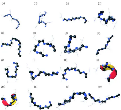
Figure 1 describes the C␣ trace of the 16 PBs we deter-mined previously. The approximation of local structures is
particularly efficient, with the mean root mean square de-viation (RMSD) of 0.58 Å. A very rough allocation into the more standard secondary structure categories would yield three-strand C-caps, two N-caps and one central -strand (PB d), four distinct coil PBs, two ␣-helix N-caps, three ␣-helix C-caps, and one central ␣-helix (PB m).
Choice of Structural Words
The transitions between successive PBs are highly specific and lead to a limited number of PB combinations. We ana-lyzed different series with PBs of different lengths. The series of five consecutive PBs had the most interesting fea-tures. One PB represents five residues, and thus five PBs represent nine residues. The sets of five PBs are, as noted above, referred to as Structural Words (SWs).
The PBs were designed on 228 proteins of the PdbSelect A protein data bank. Because of the continuous increase in the size of the Protein Data Bank (PDB; Bernstein et al. 1977; Berman et al. 2000) and the existence of various nonredundant data banks, we then assessed our description on four other data banks (culled-Pdb, PdbSelect B, SCOP, and PAPIA; see Materials and Methods and Table 1). The stability of the PBs, defined by their frequency and struc-tural meaning, did not vary significantly.
The total number of different SWs in each of the four data banks increased with the size of the data bank: fewer than
4000 SWs for PdbSelect A, roughly 8500 for culled-Pdb and PdbSelect B, 6600 for SCOP, and 9400 for PAPIA. The structural diversity of the SWs seems to increase with the number of proteins considered. It is therefore necessary to select a relatively limited number of combinations to predict structure based on reliable sequence specificity.
We defined a criterion to select the appropriate number of SWs: it is based on the ability of the selected SWs to encode a given 3D zone and is defined as the number of amino acids encoded by the SWs relative to the total number in the protein. This criterion is called coverage and is expressed as a percentage.
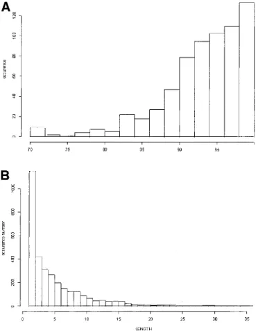
The number of SWs to be selected was thus determined by the coverage values; Figure 2 reports the variation of both. Up to 30 SWs, coverage increases markedly (60% and 80% with six and 20 SWs, respectively). Thirty SWs can encode an average of 85% of the 3D structure of any protein in the data bank. Thereafter, coverage is essentially satu-rated, regardless of the number of SWs: when the number increases from 72 to 190, coverage increases only slightly
and the curve reaches a plateau. This behavior was observed in all four data banks. Considering both sequence specificity and coverage, we selected 72 as the optimum number of SWs for prediction purposes (∼ 92%, see Fig. 3 and first column of Table 2).
Figure 4A represents the coverage distribution for all the proteins in the PAPIA data bank. Most have coverage val-ues of at least 90%. Figure 4B shows the distribution of the fragment lengths not associated with an SW in PAPIA: the mean value is 5.3 residues, and the median is 4.4. The size of the noncoded fragments is thus generally small.
The set of 72 SWs was not identical for each of the data banks, although 65 SWs appeared in all five data banks examined (see below). The remaining seven SWs had fre-quencies < 0.23% in the data banks but were are often found among the first 97 SWs (frequency > 0.13%).
Structural Words
The frequencies of the most common SWs were very simi-lar in the four simi-largest data banks and ranged from 18.4% to 16.6% (SW mmmmm), while those of the rarer words ranged from 0.21 to 0.07% (SW mmmpm). Table 3 details the frequency associated with each SW from PdbSelect A. These features were similar for the other data banks (data not shown, see Supplementary data).
The most frequent SWs are related to the principal peri-odic local structures (mmmmm and ddddd). The PBs m and
d are present at least once in 19 and 44 SWs, respectively,
related mainly to␣-helix and -sheet secondary structures.
Table 1. The five Databanks (PdbSelect A, PAPIA, culled-Pdb,
SCOP, and PdbSelect B) with the number of protein chains, the number of residues, and the number of corresponding
protein blocks Databank Protein chains Amino acids Protein blocks PdbSelect A 342 88,258 86,890 PAPIA 717 180,854 177,986 culled-Pdb 886 167,535 164,667 SCOP-ASTRAL 558 137,510 134,642 PdbSelect B 1229 238,208 235,340
Fig. 2. Variation of the coverage of SWs as a function of N (the number
of SWs selected). SWs were extracted from PdbSelect A (solid line) and PAPIA (dotted line).
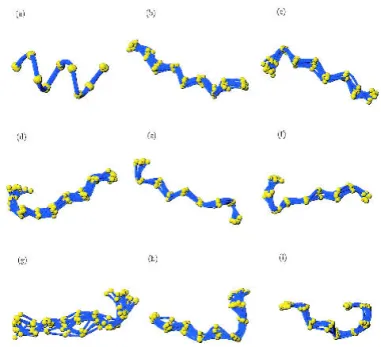
Fig. 3. Example of 3D protein fragments associated with nine Structural
Words: (a) mmmmm, (b) ddddd, (c) bccdd, (d) pacdd, (e) acddf, (f) iacdd, (g) cddfb, (h) ddfbf, and (i) dfbfk (visualization with MOLMOL software, Koradi et al. 1996).
The first SW without PB m or d is nopac, which has a frequency of 0.6%.
As expected, all of the selected SWs were overrepre-sented, but some were observed considerably more often than expected. Figure 5 reports the ratio of observed to theoretical frequency, denoted as R. This ratio ranged from 0.8 to 34. The SWs with the most significant R values are noted in Figure 5. Most of them had common roots—“dc”
and “ fk”. Interestingly, these SWs did not belong to the repetitive secondary structures.
Most of the SWs we selected were independent of the composition or size of the data bank. Nonetheless, some differences appeared, mainly for the rarer SWs; they ap-peared to depend on the data bank. For example, mmmpm,
mmmmp, and cddde are substantially less frequent in the
four most up-to-date data banks. Conversely, mmmmg, which was absent in PdbSelect A, now occurs at a frequency of almost 0.20%.
Most of the SWs overlap: the last four PBs (respectively first) of a given SW may be identical to the first four (re-spectively last) PBs of another. For example, mnopa over-laps with nopac, nopab, and nopaf. The overlapping occurs mainly in the N-caps and C-caps of SWs involving PB d, namely -strands, with for instance ccddd with bccdd,
cdddd, cdddf, and cddde. This may be due to the great
flexibility of these local structures. Overall, 55 SWs overlap on both sides with other SWs, 16 SWs overlap on one end, and only one does not overlap at all. These latter 17 SWs are less common (frequency < 0.4%).
Another interesting point is that some SWs differ by only one PB; examples are mmmmn, mmmmc, and mmmmp, or, again, nopac, nopab, and nopaf. These may correspond to a real structural transition; for example, the word nopac may evolve into nopacddd, nopab into nopabd, and nopaf into
nopafkl, or to a local structural modification, for instance, a
PB change such as that observed in mmmpm, mlmmm and
mklmm correspond to irregular␣-helices.
Structure and sequence in Structural Words
To ensure the reliability of the SWs, we calculated the val-ues of the RMSD and RMSDa root mean square deviation on angular values (RMSDa) for all of the pairs of fragments corresponding to the same SW. The RMSDa values ranged from 28° to 32°. These values are quite consistent with those computed for the five-residue fragments making up
Fig. 4. (A) Histogram of the distribution of the coverage values for the 717
protein chains from the PAPIA data bank. (B) Histogram of the distribution of the fragments not covered by the 72 SWs obtained from the PAPIA data bank.
Table 2. Coverage values obtained with the full set of SWs and the selected set (58 SWs) from the Protein Network
Databank
Covering STRIDE P-SEA PBs
SWs (%) Protein Network (%) ␣-helix(%) -sheet(%) coil (%) ␣-helix(%) -sheet(%) coil (%) ␣-helix(%) -sheet(%) coil (%) PAPIA 91.4 89.3 97.0 92.0 81.0 99.6 94.1 78.9 98.1 95.2 80.2 culled-Pdb 93.6 90.3 97.1 92.4 81.6 99.6 94.6 79.5 98.0 95.5 82.9 SCOP-ASTRAL 92.1 89.2 97.2 92.5 81.8 99.4 94.6 79.5 98.0 95.7 82.1 Pdb-select B 92.3 88.9 97.4 93.2 81.0 99.6 95.1 80.9 98.0 95.3 82.5 mean 92.4 89.4 97.2 92.5 81.4 99.6 94.6 79.7 98.0 95.4 81.9
The following two columns correspond to the repartition of coverage values of the Protein Network according to the classic secondary structures assigned with two different algorithms: STRIDE (Frishman and Argos 1995) and P-SEA (Labesse et al. 1997). The last column corresponds to the same coverage values assigned with PB m as the␣-helix, the PB d as the -sheet, and the rest as the coil state.
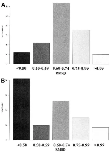
the PBs. Figure 6A reports the RMSD values for the SWs: they range from 0.34 Å to 1.11 Å (see Table 3), with an average value of 0.70 Å. Even the largest value was con-siderably smaller than those associated with coils in a three-state alphabet. Figure 6B reports the total population asso-ciated with each RMSD range. Clearly, most fragments had a small RMSD value. The largest value was for ehiac, which can be roughly described as a loop region connecting two strands. The smallest value was associated with the central zone of a periodic PB m. The SWs that include the PB m often had an RMSD less than 0.60 Å, and those including d were slightly higher (0.75 Å).
An average RMSD of 0.7 Å is a very good approximation of nine-residue fragments of 3D structures. The results are better than those for structural loop classifications (Kwasi-groch et al. 1996; Wojcik et al. 1999). The RMSD range of eight-residue loops, for example, reached 5 Å. This large discrepancy could be attributed to the remaining 10% non-encoded zones.
The amino acid propensities of the SWs, that is, the amino acid frequencies in each SW position, are extremely variable. Because of the overlapping, however, the propen-sities between SWs seem to be governed by strong and logical rules. For example, proline is overrepresented in position (+2) or (+3) of ddehi, in position (+1) or (+2) of
dehia, and in position (+1) and (0) of ehiac. Similarly,
ali-phatic hydrophobic residues are strongly underrepresented in positions (−1), (0) and (+1) of ehiac, hiacd, and iacdd. Conventional amino acid propensities were observed for the N- and C-caps of ␣-helices (Aurora and Rose 1998).
We also observed in many cases that the propensities differ from those observed for the PBs (see below). Over-lapping does not completely explain the SW propensities. For example, the underrepresentation of aliphatic hydropho-bic residues in ehiac, hiacd, and hiacdd is also found in
dehia but not in eehia.
Table 3. The 72 Structural Words used in the prediction with
their frequencies and their root mean square deviation (RMSD)
SW Obs. freq. (%) RMSd (Å) mmmmm 17.27 0.43 ddddd 3.87 1.04 lmmmm 2.45 0.34 klmmm 2.36 0.41 fklmm 2.00 0.59 cdddd 1.73 0.94 ddddf 1.38 0.82 mmmno 1.24 0.42 mmmmn 1.24 0.51 mmnop 1.09 0.63 dddfk 1.06 0.63 mnopa 1.03 0.72 dfklm 0.98 0.71 ddfkl 0.95 0.73 bdcdd 0.91 0.73 acddd 0.86 0.66 fbdcd 0.79 0.75 dddfb 0.75 0.74 ccddd 0.71 0.72 dcddd 0.70 0.74 cfklm 0.69 0.68 opacd 0.65 0.59 nopac 0.61 0.68 hiacd 0.58 0.73 ehiac 0.55 0.91 cddde 0.54 0.58 pacdd 0.54 0.83 dddde 0.54 0.80 dfbdc 0.53 0.80 dddeh 0.53 0.63 iacdd 0.52 0.51 mmmmp 0.51 0.80 ddfbd 0.47 1.11 dehia 0.43 0.81 cdddf 0.43 0.62 ddehi 0.37 1.00 bccdd 0.37 0.63 mmmpc 0.35 0.73 cdfkl 0.35 0.69 cddfk 0.30 0.76 cfbdc 0.30 0.69 kbccd 0.30 0.57 afklm 0.27 0.60 mlmmm 0.25 0.62 mklmm 0.25 0.79 bfklm 0.25 0.48 nopaf 0.25 0.40 fkbcc 0.25 0.79 cddfb 0.24 0.66 fkopa 0.23 0.74 fbfkl 0.23 0.88 ddfkb 0.22 0.66 ddfbf 0.22 1.01 fbdcf 0.22 0.73 opafk 0.22 0.67 mmpcc 0.22 1.01 dfbfk 0.22 0.64 bdcdf 0.21 0.77 mmmpm 0.21 0.51 Table 3. Continued SW Obs. freq. (%) RMSd (Å) dfkbc 0.21 0.66 pafkl 0.21 0.78 mmmmc 0.20 0.69 acddf 0.20 0.75 dfkop 0.20 0.58 dcddf 0.19 0.93 nopab 0.19 0.75 ddehj 0.19 0.67 acfkl 0.19 0.67 fklpc 0.19 0.59 abdcd 0.18 0.67 eehia 0.18 0.55 opabd 0.18 0.55
Coverage: An example
Figure 7 shows the sequence and structure of methionyl-tRNA synthetase (PDB entry: 1a8h). Coverage computed with 72 SWs for this very large protein reaches 97.4%. The nonencoded regions are split into five small zones, colored in black. They contain one to five residues and are located between repetitive structures such as pm (position 180–181) as well as in unstructured regions such as hiafe (position 141–145).
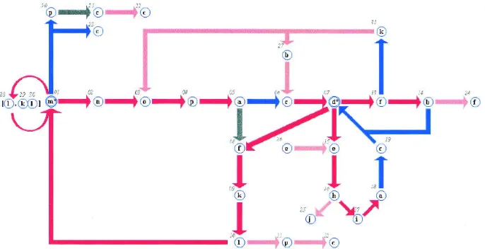
The network
The overlapping property of most of these SWs can be used to define long continuous chains. They can thus be as-sembled into a simplified network (see Materials and Meth-ods). We used the first 14 SWs to set up the network and the next 44 to supplement it. The last 14 were much more difficult to include in a simple network and have been omit-ted for clarity. Thus the network described in Figure 8 in-cludes 58 SWs (called the “network set”) that were often found in all of the data banks. This network is unique be-cause of the number of SWs and the rules for selecting it. The inclusion of other SWs according to the same rules will yield a different network.
The network summarizes all of the possible pathways followed by the backbones of all of the proteins in all of the data banks. For example, the sequence (called subgraph hereafter) m→ n→ o→ p→ a is followed by the subgraph
n→ o→ p→ a→ c. Superposition of the subgraphs completes
Fig. 6. (A) Histogram of RMSD values distribution computed between the
3D fragments associated with each of the 72 SWs (see Table 3). (B) Histogram of the frequency of fragments in a given range of RMSD values.
Fig. 5. Relative frequency R of the different 72 SWs. The value R is computed as the ratio between the observed probability pobsand the theoretical probability pth deduced from the PB frequencies considering a first-order markovian transition process. pth (SWi⳱uvwxy) ⳱ p(y| x)p(x| w)p(w| v)p(v| u)p(u) where p(y| x) is the probability that y follows x in a sequence; pobs(SWi)⳱ Nb(SWi) / NT(SW); NT(SW) is the total number of SWs in the data bank, and Nb(SWi) is the occurrence of SWi.
the graph: the subgraph in this case becomes mnopac. The graph may include branches; that is, a series may be fol-lowed by several distinct series. Thus, the subgraph mnopa is followed by two subgraphs: nopac 68% of the time and
nopaf 32%.
This network is composed of 31 nodes and uses 15 of the 16 PBs. Because of the overlap between SWs, the number of nodes is very small relative to the 58 SWs included in the network. The efficiency of the alphabet’s definition and description is shown by the ability to base a network on a selection of SWs: all of the PBs are meaningful in the de-scription of 3D protein structures. We also note that the 58 SWs defining the network are identical for all of the data-bases.
The network is based on the two periodic structures, node 01 (PB m, ␣-helix) and node 07 (PB d, -sheet). The re-petitive PBs m and d are each considered only one node turning over on itself. For example, the subgraph fk(m)xnop,
where PB m is repeated x times, corresponds to the sequence of the nodes fkl(m*)nop, with the asterisk representing the repetition of blocks. Colors represent the observed occur-rences (see Figure 8). The repetition has been mentioned before (de Brevern et al. 2000) and described with an av-erage number of repeats (anr) index, which equals 6.74 for PB m and 2.74 for PB d.
The principal entrance into helical structures is the triplet
fkl (nodes 08–09–10), and the principal exit is nop (nodes
02–03–04). There are also two shorter and rarer series: pcc (nodes 20–21–22) and c (node 23). The subgraph including node 07 (PB d) is more complex: entrance occurs only through one node, 06 (PB c). It is included in the nopac graph (nodes 02–03–04–05–06) and kbc subgraphs (nodes 31–27–06). Its most significant exit is the subgraph dehiacd (nodes 07–25–16–17–18–19–07). The next most important exit that includes node 07 is subgraph dfkl (nodes 07–08– 09–10). The more complex exit df (nodes 07–13) goes to-wards nodes 14 (PB b) and 31 (PB k).
Network coverage and Protein Blocks
We next considered the relevance and structural stability of the network. After encoding the entire set of data banks with the structural alphabet, we counted all of the protein frag-ments corresponding to SWs in the network (58); we ended up including nearly 90% of the amino acids in the structural data bank. This coverage is thus very similar to that ob-tained with the set of 72 SWs defined above.
The most interesting point is that the network contained not only the periodic structures (98% of the ␣-helices and
Fig. 7. (Left) The sequence of methionyl-tRNA synthetase from Thermus Thermophilus (code PDB 1a8h). (A) The amino acid
sequence, (B) the Protein Blocks deduced from the structure, and (C) the coverage by the SWs with the symbol (*): included and (−) not included. (Right) Visualization of the 3D backbone structure with VMD software (Humphrey et al. 1996).
95% of the-strands) but also coils, with coverage reaching 80%. Thus, most protein topologies observed in the struc-tural data bank may be described with only 58 SWs based on a simple 16-state alphabet.
Table 2 reports the coverage for each of the four up-to-date data banks, as computed with the entire set of SWs (72) and the set selected from the network (58). The values are very similar for all of the data banks, with the small differ-ences due simply to slightly different occurrence rates for each SW. Using the SWs in the network, we computed the coverage of secondary structures by the protein network. Table 2 summarizes the results for three types of secondary structures, which are, in general, difficult to assign (Colloc’h et al. 1993; Cuff and Barton 1999; de Brevern et al. 2002), and for three assignment methods. The difference between the results reflects the specificity of the assignment method. P-SEA (Labesse et al. 1997) is based on geometric criteria, whereas STRIDE (Frishman and Argos 1995) uses energetic criteria. The last assignment is based on the Pro-tein Blocks, with PBs m and d describing the core of regular secondary structures. Despite these different assignment methods, the results were very similar.
The PBs covered could be clustered into different groups: coverage of the periodic structures (PBs m and d) was ex-cellent, ranging from 95% to 99%, whereas that for their N-and C-caps ranged from 80% to 90%. The PBs with the poorest coverage were j, g, and p, with values of 58%, 69%,
and 73%, respectively. Because they are usually present in long loops, they are not often found in the protein network. Most of the residues (90%) in the data bank are thus included in the network. The main doublets not included are
bd and fb. The triplet fbd (more than 500 occurrences in
PdbSelect A) is included in the network (nodes 13–14–07) but is found with 413 occurrences in SWs not considered among the 72 selected SWs. The PBs located at the N- and C-ends of this triplet vary greatly, and thus probably few sequences of five consecutive blocks were considered in the network.
Words and 3D stability
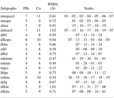
The structural alphabet was developed to approximate the three-dimensional structure of 5 C␣ locally, and the network uses overlapping sequences of five PBs (i.e., 9 C␣). It is therefore important to verify whether these local approxi-mations with average values still yield similar protein frag-ments. We extracted from the 58-SW network 17 subgraphs (i.e., series of sequential nodes), which were from four to seven PBs long (i.e., 8 to 11 C␣) and covered the network entirely. The average RMSD and RMSDa were calculated for all pairs of protein fragments in the data bank that cor-responded to the same subgraph (Table 4). Then we looked for possible structural subfamilies in the subgraphs, that is, distinct local folds associated with the same PB sequence.
Fig. 8. The protein network composed of 31 nodes. Each node is labeled with the PB letter and its own number. The colors depend
on the occurrence rates: red, > 10% of the protein structural data bank; blue, between 10% and 6%; gray, between 6% and 3.5%; and pink, less than 3.5%. Nodes 01 and 07 represent Protein Blocks m and d, respectively. Their repetition (anr of 6.74 and 2.74, respectively) is symbolized with a double circle and a star (m* and b*). Node 28 (PB l) and nodes 29–30 (PBs k and l) are included in the mlm and mklm sequences. The network is discontinuous, and thus nodes 12, 22, and 23 (PB c), node 25 (PB j), and node 24 (PB
PBs are defined on the basis of the RMSDa. All 17 sub-graphs had an average RMSDa value close to 30 degrees (with a Gaussian distribution; data not shown). This value is similar to that chosen for defining individual PBs, although the number of angles involved was high (14 to 20) for the subgraphs. A clustering procedure with two or three groups was applied for each subgraph (see Materials and Methods). The average RMSDa for each cluster was quite similar to the value found before clustering. We searched for specific positions among the angle signals in the subgraph with the greatest variability. The (,) signals were well conserved for most of the words.
We calculated the mean C␣ RMSD for the same pairs of fragments for which we calculated the RMSDa. The C␣ superimposition of the fragments showed remarkable con-sistency: the average RMSD for most subgraphs was close to 0.66 Å (see Table 3). Figure 9A illustrates the subgraph
dfkopa (nodes 07–13–31–03–04–05), which has an RMSD
of 0.64 Å for a length of 8 C␣. In this example, all of the fragments—for both periodic and nonperiodic regions— were well-approximated structures. Figures 9B and C su-perimpose fragments from the subgraphs dehiacd (nodes 07–15–16–17–18–19–07) and mnopacd (nodes 01–02–03– 04–05–06–07). Their respective RMSD values were 1.02 Å and 0.61 Å, both for a length of 11 C␣. After the subgraphs were clustered, the RMSD, like the RMSDa, remained quite similar to that observed for the entire set.
On the whole, the 3D folds appeared similar for all of the fragments associated with a given subgraph. In conclusion, the network ensured an accurate structural description and reasonable structural variability as well as accurate
approxi-mation of the local 3D structure of long fragments. These results are similar to those previously reported for long loops (Wintjens et al. 1996; Boutonnet et al. 1998) but, unlike those studies, we did not use any a priori definition of secondary structure.
Amino acid specificity
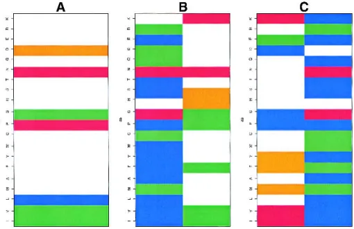
The amino acid distributions in the nodes have several in-teresting properties. We observed three different cases. In
Table 4. The 17 subgraphs (protein fragments) used to test the
structural stability of the simplified network with the associated SW series, the number of PBs, the number of associated C␣, and the corresponding nodes
Subgraphs PBs C␣ RMSd (Å) Nodes mnopacd 7 11 0.61 01 - 02 - 03 - 04 - 05 - 06 - 07 mnopa 5 9 0.72 01 - 02 - 03 - 04 - 05 ehiac 5 9 0.91 15 - 16 - 17 - 18 - 19 dehiacd 7 11 1.02 07 - 15 - 16 - 17 - 18 - 19 - 07 dfbf 4 8 0.59 07 - 13 - 14 - 24 dfkopa 6 10 0.64 07 - 13 - 31 - 03 - 04 - 05 fklm 4 8 0.66 07 - 13 - 14 - 24 afkl 4 8 0.58 05 - 08 - 09 - 10 dfbd 4 8 0.75 07 - 13 - 14 - 07 mklmm 5 9 0.47 01 - 29 - 30 - 01 - 01 mlmm 4 8 0.49 01 - 28 - 01 - 01 mpcc 4 8 0.15 01 - 20 - 21 - 22 fklpc 5 9 0.75 08 - 09 - 10 - 11 - 12 eehiac 6 10 0.54 26 - 15 - 16 - 17 - 18 - 19 dehj 4 8 0.67 07 - 15 - 16 - 25 dfkbc 5 9 1.01 07 - 13 - 31 - 27 - 06 dfklm 5 9 0.71 07 - 08 - 09 - 10 - 01
Fig. 9. 3D superimpositions of protein fragments associated with different
subgraphs (cf. Table 4) (A) dfkopa (nodes 07–13–31–03–04–05), (B)
dehiacd (nodes 07–15–16–17–18–19–07), and (C) mnopacd (nodes 01–
the first, the amino acid distribution of a node was very similar to that of the PB corresponding to this node: PB and node had almost identical amino acid over- and underrep-resentations. In the second case, there were some qualitative differences, but for only one or two amino acids. In the third case, the distribution in the node is quite distinct from that in the PB (i.e., most of the amino acids behave drastically differently). Node 16 (PB h, Fig. 10A) is an example of the first situation: it is involved in six different SWs, and the distribution of amino acids is similar to the average distri-bution observed in the central position of PB h. The same behavior is observed for node 17 (PB i), node 25 (PB j), and node 02 (PB n).
Substantially different occurrence rates prevent the easy comparison of some PBs involved in different nodes. Hence, the amino acid distribution in node 06 (PB c) is similar to that in PB c, and this node represents 68% of the PB c included in the network, whereas nodes 12, 19, 21, 22, and 23 never account for more than 10% of the occurrences of PB c. Nodes 14 (78%) and 27 (22%), both PB b, were well represented. Proline is underrepresented in node 14 but strongly overrepresented in PB b. The relative absence of proline in node 14 is counterbalanced by an overrepresen-tation of glycine that may have similar structural conse-quences. Figures 10B and C provide two examples of strong divergences for the same PB within two different nodes. The characteristics of nodes 04 and 20 (PB p, Fig. 10B) are rather distantly related: node 4 is very similar to PB p, whereas node 20 differs quite substantially, with overrep-resentations of histidine, serine, and lysine. Nodes 05 and 18 (PB a, Fig. 10C) are also very different. The distribution in
node 05 is similar to that in the PB a distribution but with more pronounced overrepresentations (isoleucine, valine, lysine), whereas the distribution in node 18 is almost the inverse, with strong underrepresentations of these amino acids and a strong propensity for glycine and aspartate that was not observed in the original PB.
Relation between Structural Words and so-called loops
In some ways, the SWs can be compared to additional states introduced to define more precisely some local motifs as-sociated with the “coil” states of the three-state alphabet. Hence, 50% of the type I turns extracted from the complete Protein Data Bank (nearly 15,000 entries) are represented by a PB k that is always close to a PB m in subgraphs fklm (nodes 08–09–10–01) or mklm (nodes 01–29–30–01). Simi-larly, 80% of type II turns end with ia, and more than half of those are in the network, in the subgraph ehia (nodes 15–16–17–18). Type III turns, like type I turns, are always near PB m, so that 80% of them are characterized by the subgraph lm (nodes 10–01/29–01) and more than 60% by
klm (nodes 09–10–01/29–30–01). The network thus allows
these turns to be found, but does not connect them directly to secondary structures.
Structure prediction
The Bayesian approach with PBs yielded an initial predic-tion rate of 34% (de Brevern et al. 2000). Predicpredic-tion fea-tures, however, may be strongly influenced by amino acid specificity, which may not be the same in SWs as in PBs
Fig. 10. Z-scores of the amino acid distribution: (A) node 16 (PB h), (B) nodes 04 and 20 (PB p), and (C) nodes 05 and 18 (PB a).
Z-scores less than −4.4 are in blue, Z-scores between −4.4 and −1.96, in green, Z-scores between −1.96 and +1.96, in white, Z-scores between +1.96 and +4.4 in orange and more than 4.4, in red. The amino acids are defined on the vertical axis in the order IVLMAFYWCPGHSTNQDERK.
alone. We therefore decided to test how SWs affected pre-diction. To do so, we used one half of a data bank to per-form the learning step, and the other half for the validation. With PdbSelect A (342 proteins: 228 in the training set and 114 in the validation) and 72 SWs instead of 16 PBs, the prediction rate increased by 4%. We repeated this test with the PAPIA (358 and 359 proteins) and culled-Pdb (443 and 443 proteins) data banks and obtained very similar results. Globally, the prediction rate was 38.5% for the learning set and 38% for the validation set.
Figure 11 reports an example for both prediction ap-proaches (PB-based and SW-based) applied to ubiquitin-conjugating enzyme (PDB code: 1aak, 144 residues). Use of the latter approach improved the prediction rate from 30.5% to 41.0%. Both approaches predicted 25 sites in common; use of PBs predicted an additional 17, and SWs an addi-tional 31. The predictions with SWs also provided longer regions. They are thus clearly interesting for local structure prediction. These results are perfectly representative of the results obtained for the proteins tested (from 114 to 443 proteins, according to data bank).
Discussion
Analysis of a structural data bank encoded in Protein Blocks shows that some PB sequences are common and strongly interdependent. They allow us to construct a simple directed graph that logically connects the most frequent five-PB se-ries. The network contains 90% of the five protein structural data banks we tested. More than 80% of the “variable” regions of coils are described with very good 3D accuracy. This network shows that coils can be described more pre-cisely with a new categorization that is not based on the standard three-state alphabet (␣-helix, -sheet, and every non-␣ and non-). We tested this method with five different data banks, constituted with different approaches, and ob-tained very similar final results.
This approach thus has some advantages over the tradi-tional methods based on motifs of constant size connecting
two repetitive structures (Wojcik et al. 1999), especially because the definition of terminal ends of repetitive struc-tures is far from optimal (Cuff and Barton 1999). This un-certainty about the ends may result in nearby 3D loop con-formations being considered to belong to different structural groups. Moreover, this network shows, as Ring and cowork-ers (Ring et al. 1992) have already reported, that loops can be described as composed of series. In our case, SWs cor-respond to 9 C␣, and most of the regions covered include at least seven SWs (thus 15 C␣). Accordingly, this approach is quite interesting for loops and could be usefully applied in molecular modeling.
Two final points require discussion: (1) is the number of PBs used to define SWs appropriate? and (2) is the number of SWs relevant? The results obtained here indicate that the response to both questions is affirmative. First, a length of five PBs makes it possible to describe long fragments (9 C␣) while accurately approximating most of the local pro-tein folds. Second, the use of 72 SWs allows us to describe most (90%) of the local protein folds. Doubling the number of SWs improved coverage by only 1%; in addition, the sequence-structure specificity falls rapidly for the least common SWs and is not useful for prediction.
Various improvements may increase the prediction rate. For example, at the C-terminal end of the ubiquitin-conjugating enzyme (Fig. 11), the predicted blocks are
mmmlmopamdmdmmbff. Prediction based solely on PBs
found none of the last 17 PBs, whereas SW-based prediction found eight of them. Similarly, a filtering approach might prevent such unlikely situations as a d block surrounded by
m blocks (roughly, an amino acid in a conformation close to
a strand enclosed in a helical region). Some errors in local prediction may thus be detected and corrected.
Even a simple alphabet, then, allows the identification of connected zones that are structurally similar in different proteins. Analysis of the amino acid frequency reveals sig-nificant sequential differences that can be useful in predic-tion methods. The improvement in the Bayesian predicpredic-tion must be compared with secondary structure analysis that takes sequentiality into account (Bystroff et al. 2000).
Fig. 11. Prediction of the ubiquitin-conjugating enzyme (PDB code: 2aak): TRUE: the 3D structure encoded in terms of PBs. P. PB:
Prediction with a Bayesian probabilistic approach based on the amino acid specificity of the PBs. (Prediction rate: 30.5% [de Brevern et al. 2000].) P. SW: Prediction with a Bayesian probabilistic approach based on the amino acid specificity of the SWs (prediction rate: 41%). Cons: Agreement and discrepancies of the two sets of prediction results compared with the PB assignment (−) no true PB found, (䡩) true PB only found with P. PB, (䊊) true PB only found with P. SW and (多) true PB found with both approaches.
Clearly the gap between local and global 3D prediction remains. Nevertheless, simple local alphabets introduced as local constraints have shown their usefulness for improving ab initio predictions (Simons et al. 1999; Bonneau et al. 2001). Compared to similar approaches such as I-sites (Bystroff and Baker 1998; Bystroff et al. 2000), the set of structural words we propose combines sequence specificity and overlapping features; it therefore leads to logical path-ways that connect the SWs. These pathpath-ways are currently being examined in a new prediction method.
Finally, an important feature of the network is that it can translate the 3D structure of a protein simply but more ac-curately than the three-state alphabet. This simplified infor-mation could be very helpful for future classification of 3D folds, fast and efficient comparison of 3D structures, and searching for distant but nevertheless homologous se-quences that share similar folds. This network could be easily compared to a Markov chain but one with no a priori distribution laws.
Material and methods Protein Blocks
We previously described a set of 16 small protein fragments 5 C␣ long, called Protein Blocks (PBs; de Brevern et al. 2000). They were obtained by an unsupervised classifier similar to Kohonen Maps (Kohonen 1982, 2001) and Hidden Markov Models (Rabiner 1989). The 5 C␣ fragments are encoded in (⌽, ⌿)vectors. Figure 1 presents all 16 PBs (a–p). PBs a to f appear to be related to the -sheet secondary structure: d corresponds to the more regular central part, a, b, and c to the N-cap, and e and f to the C-caps. PBs
k to p may be related to the␣-helix secondary structure, with PB m for the central part of a right helix, k and l for the N-caps, and n, o, and p for the C-caps. Blocks g through j may be associated
mainly with coil structures. The set of 16 PBs compose a structural alphabet that efficiently approximates the local protein backbone. The amino acid specificity within these PBs enabled us to propose a new method for predicting 3D local protein structures (de Brev-ern et al. 2000).
Protein data banks and encoding
The protein coding is composed of different successive states: (1) The protein is coded as a sequence of⌽-⌿ dihedral angles, so that a protein L amino acids long is defined by a signal of 2(L−1) dihedral angular values. (2) Each fragment of M residues (M⳱5) centered at the␣-carbon C␣nis represented by a vector of eight
dihedral angles composed of ⌿n−2, ⌽n−1, ⌿n−1, ⌽n, ⌿n, ⌽n+1,
⌿n+1, and ⌽n+2. The fragment is compared to each PB with a
dissimilarity measure named the RMSDa (root mean square de-viations on angular values) and defined as the Euclidean distance of the 2(M−1) values. The lowest RMSDa value determines the assignment of the PB.
The 3D-protein structure data bank (Protein Data Bank or PDB, Bernstein et al. 1977; Berman et al. 2000) contains more than 15,000 entries. Because many are very similar for sequence and/or structure, it is necessary to use a nonredundant data bank. PBs were first defined from a data bank containing 342 chains,
ex-tracted from the 1998-PDBselect data bank (Hobohm et al. 1992; Hobohm and Sander 1994), and taking into account only the X-ray structures established with a resolution of less than 2.5 Å and sequences sharing less than 25% identity. Each chain was carefully examined with geometric criteria to avoid bias from zones with missing density. The data bank is denoted here as PdbSelect A. In the present work, we considered different data banks to take into account the considerable increase in available 3D structures.
All computations were performed with four different data banks. The first (denoted PAPIA) is based on the PAPIA/PDB-REPRDB database (Noguchi et al. 2001); we selected the chains with a resolution of 2 Å or less and an R-factor less than 0.2. Each selected structure has an RMSD value larger than 10 Å from all of the representative chains and a sequence identity no higher than 30%. The second data bank is the culled-Pdb (Dunbrack 2001), reexamined with the same structural parameters (resolutionⱕ to 2 Å, R-factor less than 0.2), but with a sequence identity threshold fixed at 20%. It is denoted culled-Pdb. The third data bank comes from the famous SCOP data bank established from a manual fold classification (Murzin et al. 1995). We examined it with ASTRAL software (Brenner et al. 2000) and selected structures with a se-quence identity threshold of 30%. Each fold is thus represented by one protein. This data bank is denoted SCOP. Finally the fourth data bank was the last version of Pdb-select (Hobohm et al. 1992; Hobohm and Sander 1994). The selection criteria were identical to those for PdbSelect A. We considered only the X-ray structures. It is denoted PdbSelect B. In all cases, we systematically checked the continuity of the backbone structure with geometric parameters, such as chemical bond lengths. When the bonds were larger than a given threshold, the protein was divided into as many subchains as necessary.
In all cases, proteins (or protein chains or subchains) were di-vided into fragments of five successive residues. The fragments overlapped, so that each protein of lengthL was encoded with L−4 fragments. Hence the 88,258 residues of PdbSelect A, containing 342 proteins, correspond to 86,890 fragments, translated into 86,890 PBs. Table 1 summarizes the composition of the five data banks. The four new data banks include between 137,510 and 238,208 residues.
The amino acid composition was very similar for all five data banks.
Structural Words
Our goal was to characterize the possible relations between the most frequent series of PBs observed in a data bank of protein structures. Once we encoded the data bank in terms of PBs, we examined the most frequent series of five PBs, corresponding to nine consecutive residues. If we considered all of the different series that occur, we would cover all of the protein substructures but would have to deal with a huge number of series, most of which occur at a very low frequency. The sequence-structure re-lationship that could be deduced for these series would thus be statistically biased. To represent both a large 3D spectrum of local structures and a sufficiently accurate 1D-3D relationship, it is nec-essary to select the most frequent series, and thus only a limited number. After various experiments, we observed that, on average, 90% of the 3D structure of any protein can be represented with at most 72 different series. This indicator is called “coverage” herein. Each element of the series defines a so-called “Structural Word” (SW). The frequency of each SW differs according to the database used. In the case of the PBs from data bank PdbSelect A, the last SW is observed 150 times. The properties of the SWs were
reas-sessed within the four largest data banks (see above) to assess the relevance of the selected SWs.
All of the structural fragments associated with the same SW were optimally superimposed. The RMSD and RMSDa values were computed to estimate the structural variability of each SW. The C␣ RMSD was computed along the nine residues; the RMSDa included the (⌿i,⌽i+1) vectors with i⳱1 to 8 describing the SW.
Note that the fragments are overlapping, so that each protein of lengthL is encoded with L−8 SWs.
Network conception
The relationship between the series of PBs defining the SWs may be expressed by a simple directed graph. A graphG corresponds to
V nodes (“vertices”) and E segments (“edges”) that connect the
nodes. The graph is directed if each segment has only one direc-tion,G (V, E). In our study, each node Viis characterized by one
PB, and each link Eicorresponds to a transition between two PBs.
A sequence of five blocks is represented by a directed subgraph. For example, the subgraph m→ n→ o→ p→ a→ c is described by the SW mnopa going to c. The construction of the network is the combination of subgraphs composed of SWs: (v1→ v2→ v3→
v4→ v5) and (v2→ v3→ v4→ v5-→ v6) will become (v1→ v2→
v3→ v4→ v5→ v6). The network is noncontinuous; its only rule is
to find five consecutive PBs included in the network, that is, an SW.
Structural stability of the network
The network is based on the most frequent Structural Words. The important question involves the relevance of our protein network: does the combination of SWs observed in the network lead to incompatible 3D local structures or, inversely, do we observe 3D stability along combinations of frequently observed SWs.
To insure the structural stability of the network, we chose 17 subgraphs (i.e., series of nodes from four to seven PBs long) included in the network and covering it entirely. We extracted all of the protein fragments from the structural data bank associated with each of the 17 subgraphs and superimposed, pairwise, all of the protein fragments extracted from each. The corresponding RMSD values were then clustered in two or three groups, hierar-chically. The mean RMSD was calculated for each cluster and compared to the global average RMSD to determine whether a cluster could be assigned to a more specific local fold or not. Similar computations were performed with RMSDa measures. Z-score
The amino acid occurrences for a given node were normalized into a Z-score⳱ (nobserved
(i,x) − ntheoretical
(i,x)) /√ ntheoretical
(i,x), with nobserved
(i,x) the number of times amino acid i is observed in node
x, and ntheoretical
(i,x) the number expected. The product of the occurrence of node x with the frequency of amino acid i in the entire data bank equals ntheoretical
(i,x). Positive Z-scores (respec-tively negative) correspond to overrepresented amino acids (re-spectively underrepresented) in node x; threshold values of 4.4 and 1.96 were chosen, that is, a probability p less than 10−5
and 10−3
. Prediction of SWs by a Bayesian
probabilistic approach
The goal was to predict the optimal PB for each position along a sequence of length L. To this end, we used a Bayesian probabilistic
approach similar to that proposed in a previous work (de Brevern et al. 2000). In the present work, we focused on the conditional probability of observing the SWkgiven an amino acid chain X, (a1,
a2,. . ., al), denoted P(SWk| X). Bayes’ theorem accomplishes the
inversion of the sequence X and the structure SWk. This leads to:
P(X| SWk)⳱ P(a1| SWk) × P(a2| SWk) ×. . . .× P(al| SWk)
A window of length l (l⳱15 here) slides along the sequence, centered on a position s.
To define the optimal Structural Words SW* for a given amino acid fragment X around a site s in a protein, we used the prediction score Rk:
Rk⳱ P (X | SWk) / P(X)⳱ P(SWk| X) / P(SWk)
The ratio Rkmeasures the information provided by knowledge
of the amino acid chain X in predicting Structural Word SWk. The
criterion is equivalent to a likelihood ratio. The optimal structural block of the 72 possible blocks, SWk, is defined as SW* ⳱
argmax{Rk}. The central PB of SW* is then assigned to the central
residue of the chain X. The final prediction rate is the ratio between the number of PBs correctly predicted and all of the PBs of the protein.
To assess the predictions, the data bank was divided into two equal sets, one to define the SWs with the corresponding sequence-structure relationship P(SWk | X), and the other to perform the
predictions. All of the sequences in this set have been so treated. Electronic supplemental material
Frequencies of each SW in the five databanks.
Acknowledgments
This work was supported by a grant from the Ministe`re de la Recherche and from “Action Bioinformatique inter EPST” number 4B005F. A.dB. is supported by a grant from the Fondation de la Recherche Me´dicale. We also acknowledge the constructive com-ments of the referees.
The publication costs of this article were defrayed in part by payment of page charges. This article must therefore be hereby marked “advertisement” in accordance with 18 USC section 1734 solely to indicate this fact.
References
Aurora, R. and Rose, G.D. 1998. Helix capping. Protein Sci. 7: 21–38. Baker, D. and Sali, A. 2001. Protein structure prediction and structural
genom-ics. Science 294: 93–96.
Barlow, D.J. and Thornton, J.M. 1988. Helix geometry in proteins. J. Mol. Biol.
201: 601–619.
Berman, H.M., Westbrook, J., Feng, Z., Gilliland, G., Bhat, T.N., Weissig, H., Shindyalov, I.N., and Bourne, P.E. 2000. The protein data bank. Nucleic
Acids Res. 28: 235–242.
Bernstein, F.C., Koetzle, T.F., Williams, G.J., Meyer, Jr., E.F., Brice, M.D., Rodgers, J.R., Kennard, O., Shimanouchi, T., and Tasumi, M. 1977. The protein data bank: A computer-based archival file for macromolecular struc-tures. J. Mol. Biol. 112: 535–540.
Bonneau, R. and Baker, D. 2001. Ab initio protein structure prediction: Progress and prospects. Annu. Rev. Biophys. Biomol. Struct. 30: 173–189. Bonneau, R., Tsai, J., Ruczinski, I., Chivian, D., Rohl, C., Strauss, C.E.M., and
Baker, D. 2001. Rosetta in CASP4: Progress in ab initio protein structure prediction. Proteins 37(S5): 119–126.
Boutonnet, N.S., Kajava, A.V., and Rooman, M.J. 1998. Structural classifica-tion of␣ and ␣ supersecondary structure units in proteins. Proteins
30: 193–212.
Brenner, S.E., Koehl, P., and Levitt, M. 2000. The ASTRAL compendium for sequence and structure analysis. Nucleic Acids Res. 28: 254–256.
Bystroff, C. and Baker, D. 1998. Prediction of local structure in proteins using a library of sequence-structure motif. J. Mol. Biol. 281: 565–577. Bystroff, C., Thorsson, V., and Baker, D. 2000. HMMSTR: A hidden Markov
model for local sequence-structure correlations in proteins. J. Mol. Biol.
301: 173–190.
Camproux, A.C., Tuffery, P., Chevrolat, J.P., Boisvieux, J.F., and Hazout, S. 1999. Hidden Markov model approach for identifying the modular frame-work of the protein backbone. Protein Eng. 12: 1063–1073.
Camproux, A.C., de Brevern, A.G., Hazout, S., and Tuffery, P. 2001. Exploring the use of a structural alphabet for a structural prediction of protein loops.
Theor Chem Acc 106(1/2): 28–35.
Chan, A.W., Hutchinson, E.G., Harris, D., and Thornton, J.M. 1993. Identifi-cation, classifiIdentifi-cation, and analysis of-bulges in proteins. Protein Sci. 2: 1574–1590.
Chandonia, J.M. and Karplus, M. 1999. New methods for accurate prediction of protein secondary structure. Proteins 35: 293–306.
Chou, K.C. 1997. Prediction and classification of␣-turn types. Biopolymers 42: 837–853.
Colloc’h, N., Etchebest, C., Thoreau, E., Henrissat, B., and Mornon, J.-P. 1993. Comparison of three algorithms for the assignment of secondary structure in proteins: The advantages of a consensus assignment. Protein Eng. 6: 377–382. Cuff, J.A. and Barton, G.J. 1999. Evaluation and improvement of multiple sequence methods for protein secondary structure prediction. Proteins 34: 508–519.
de Brevern, A.G. and Hazout, S. 2000. Hybrid Protein Model (HPM): A method to compact protein 3D-structures information and physicochemical proper-ties. IEEE Comp Soc. S1: 49–54.
———. 2001. Compacting local protein folds by a “Hybrid Protein Model.”
Theor Chem Acc 106(1/2): 36–47.
———. 2002. Improvement of “Hybrid Protein Model” to define an optimal repertory of contiguous 3D protein structure fragments. Bioinformatics (in press).
de Brevern, A.G., Etchebest, C., and Hazout, S. 2000. Bayesian probabilistic approach for predicting backbone structures in terms of protein blocks.
Proteins 41: 271–287.
de Brevern, A.G., Camproux, A.C., Hazout, S., Etchebest, C., and Tuffery, P. 2001. Beyond the secondary structures: The structural alphabets. In Recent
Advances In Protein Engineering (ed. S.G. Pandalai), Vol. 1, pp. 319–331.
Research Signpost, Trivandrum, India.
Dunbrack Jr., L. 2001. http://www.fccc.edu/research/labs/dunbrack/pisces/ culledpdb.html
Fetrow, J.S. 1995. Omega loops: Nonregular secondary structures significant in protein function and stability. FASEB J. 9: 708–717.
Fetrow, J.S., Palumbo, M.J., and Berg, G. 1997. Patterns, structures, and amino acid frequencies in structural building blocks, a protein secondary structure classification scheme. Proteins 27: 249–271.
Fiser, A. and Sali, A. 2001. MODELLER: Generation and refinement of ho-mology models. Methods Enzymol. (in press).
Frishman, D. and Argos, P. 1995. Knowledge-based protein secondary structure assignment. Proteins 23: 566–579.
Genome International Sequencing Consortium. 2000. Initial sequencing and analysis of the human genome. Nature 409: 860–921.
Hobohm, U. and Sander, C. 1994. Enlarged representative set of protein struc-tures. Protein Sci. 3: 522–524.
Hobohm, U., Scharf, M., Schneider, R., and Sander, C. 1992. Selection of a representative set of structures from the Brookhaven Protein Data bank.
Protein Sci. 1: 409–417.
Humphrey, W., Dalke, A. and Schulten, K. 1996, VMD—Visual molecular dynamics. J. Mol. Graph. 14: 33–38.
Hutchinson, E.G. and Thornton, J.M. 1994. A revised set of potentials for-turn formation in proteins. Protein Sci. 3: 2207–2216.
Jaroszewski, L., Rychlewski, L., Zhang, B., and Godzik, A. 1998. Fold predic-tion by a hierarchy of sequence, threading, and modeling methods. Protein
Sci 7: 1431–1440.
Jones, D.T., Tress, M., Bryson, K., and Hadley, C. 1999. Successful recognition of protein folds using threading methods biased by sequence similarity and predicted secondary structure. Proteins S3: 104–111.
Kelley, L.A., MacCallum R.M., and Sternberg, M.J. 2000. Enhanced genome annotation using structural profiles in the program 3D-PSSM. J. Mol. Biol.
299: 499–520.
Kohonen, T. 1982 Self-organized formation of topologically correct feature maps. Biol. Cybern. 43: 59–69.
———. 2001. Self-organizing maps, 3rd ed., chapters 2–4. Springer-Verlag, Berlin, Germany.
Koradi, R., Billeter, M., and Wüthrich, K. 1996. MOLMOL: A program for display and analysis of macromolecular structures. J. Mol. Graph. 14: 51–55. Kumar, S. and Bansal, M. 1998. Geometrical and sequence characteristics of
␣-helices in globular proteins. Biophys J. 75: 1935–1944.
Kwasigroch, J.-M., Chomilier, J., and Mornon, J.-P. 1996. A global taxonomy of loops in globular proteins. J. Mol. Biol. 259: 855–872.
Labesse, G., Colloc’h, N., Pothier, J., and Mornon, J.-P. 1997. P-SEA: A new efficient assignment of secondary structure from C␣ trace of proteins.
Com-put. Appl. Biosci. 13: 291–295.
Leszczynski, J.F. and Rose, G.D. 1986. Loops in globular proteins: A novel category of secondary structure. Science 14: 849–855.
Meller, J. and Elber, R. 2001. Linear programming optimization and a double statistical filter for protein threading protocols. Proteins 45: 241–261. Milner-White, E.J. 1988. Recurring loop motif in proteins that occurs in
right-handed and left-right-handed forms. Its relationship with␣-helices and -bulge loops. J. Mol. Biol. 199: 503–511.
Murzin A.G., Brenner S.E., Hubbard T., and Chothia, C. 1995. SCOP: A struc-tural classification of proteins database for the investigation of sequences and structures. J. Mol. Biol. 247: 536–540.
Noguchi, T., Matsuda, H., and Akiyama, Y. 2001. PDB-REPRDB: A database of representative protein chains from the Protein Data Bank (PDB). Nucleic
Acids Res. 29: 219–220.
Orengo, C.A., Bray, J.E., Hubbard, T., LoConte, L., and Sillitoe, I. 1999. Analy-sis and assessment of ab initio three-dimensional prediction, secondary structure, and contacts prediction. Proteins 37: 149–170.
Ouali, M. and King, R.D. 2000. Cascaded multiple classifiers for secondary structure prediction. Protein Sci. 9: 1162–1176.
Pavone, V., Gaeta, G., Lombardi, A., Nastri, F., Maglio, O., Isernia, C., and Saviano, M. 1996. Discovering protein secondary structures: Classification and description of isolated␣-turns. Biopolymers 38: 705–721.
Petersen, T.N., Lundegaard, C., Nielsen, M., Bohr, H., Bohr, J., Brunak, S., Gippert, G.P., and Lund, O. 2000. Prediction of protein secondary structure at 80% accuracy. Proteins 41: 17–20.
Pollastri, G., Przybylski, D., Rost, B., and Baldi, P. 2002. Improving the pre-diction of secondary structure in three and eight classes using recurrent neural networks and profiles. Proteins 47: 228–235.
Rabiner, L.R. 1989. A tutorial on Hidden Markov Models and selected appli-cations in speech recognition. Proc. IEEE 77: 257–285.
Rajashankar, K.R. and Ramakumar, S. 1996. turns in proteins and peptides: Classification, conformation, occurrence, hydratation and sequence. Protein
Sci. 5: 932–946.
Richardson, J.S. 1981. The anatomy and taxonomy of protein structure. Adv.
Protein Chem. 34: 167–339.
Richardson, J.S., Getzoff, E.D., and Richardson, D.C. 1978. The bulge: A common small unit of nonrepetitive protein structure. Proc. Natl. Acad. Sci.
75: 2574–2578.
Ring, C.S., Kneller, D.G., Langridge, R., and Cohen, F.E. 1992. Taxonomy and conformational analysis of loops in proteins. J. Mol. Biol. 224: 685–699. Rohl, C.A. and Doig, A.J. 1996. Models for the 310-helix/coil,-helix-coil and
␣-helix/310-helix/coil transitions in isolated peptides. Protein Sci. 5: 1689–
1696.
Rooman, M.J., Rodriguez, J., and Wodak, S.J. 1990. Automatic definition of recurrent local structure motifs in proteins. J. Mol. Biol. 213: 327–336. Rose, G.D., Gierasch, L.M., and Smith, J.A. 1985. Turns in peptides and
pro-teins. Adv. Protein Chem. 37: 1–109.
Rost, B. 2001. Review: Protein secondary structure prediction continues to rise.
J. Struct. Biol. 134: 204–218.
Rost, B. and Sander, C. 1993. Prediction of protein secondary structure at better than 70% accuracy. J. Mol. Biol. 232: 584–599.
Salamov, A.A. and Solovyev, V.V. 1997. Protein secondary structure prediction using local alignments. J. Mol. Biol. 268: 31–36.
Sali, A. and Blundell, T.L. 1993. Comparative protein modelling by satisfaction of spatial restraints. J. Mol. Biol. 234: 779–815.
Schuchhardt, J., Schneider, G., Reichelt, J., Schomburg, D., and Wrede, P. 1996. Local structural motifs of protein backbones are classified by self-organiz-ing neural networks. Protein Eng. 9: 833–842.
Sibanda, B.L. and Thornton, J.M. 1991. Conformation of hairpins in protein structures: Classification and diversity in homologous structures. Methods
Enzymol. 202: 59–82.
Simons, K.T., Kooperberg, C., Huang, E. and Baker, D. 1997. Assembly of protein tertiary structures from fragments with similar local sequences using simulated annealing and Bayesian scoring functions. J. Mol. Biol. 268: 209–225.
Simons, K., Bonneau, R., Ruczinski, I., and Baker, D. 1999. Ab initio protein structure prediction of CASP III targets using ROSETTA. Proteins 37: 171–176.
Unger, R., Harel, D., Wherland, S., and Sussman, J.L. 1989. A 3D building blocks approach to analyzing and predicting structure of proteins. Proteins
5: 355–373.
Wilmot, C.M. and Thornton, J.M. 1988. Analysis and prediction of the different types of-turn in proteins. J. Mol. Biol. 5: 221–232.
Wintjens, R.T., Rooman, M.J., and Wodak, S.J. 1996. Automatic classification and analysis of␣ ␣-turn motifs in proteins. J. Mol. Biol. 255: 235–253. Wojick, J., Mornon, J.-P., and Chomilier, J. 1999. New efficient
statis-tical sequence-dependent structure prediction of short to medium-sized pro-tein loops based on an exhaustive loop classification. J. Mol. Biol. 289: 1469– 1490.
Xu, Y. and Xu, D. 2000. Protein threading using PROSPECT: Design and evaluation. Proteins 40: 343–354.