Contraction maps and applications to the analysis of iterative algorithms

Contraction Maps and Applications to the Analysis of

Iterative Algorithms

by

Emmanouil Zampetakis

Submitted to the Department of Electrical Engineering and Computer Science

in partial fulfillment of the requirements for the degree of

Master of Science

at the

MASSACHUSETTS INSTITUTE OF TECHNOLOGY

February 2017

@

Massachusetts Institute of Technology 2017. All rights reserved.

Signature redacted

Author...

Department of Ele/ rical Engineering and

Computer Science

January 31, 2017

Certified by

...

Signature

redacted

...

Constantinos Daskalakis

Associate Professor EECS

Thesis Supervisor

Accepted by ...

Signature redacted

I /

&U(

_{Professor Leslie A. Kolodziejski}

MASSACHUSETTS INSTITUTE

0F

T

HNOLOGY

MAR 13 2017

LIBRARIES

Contraction Maps and Applications to the Analysis of Iterative

Algorithms

by

Emmanouil Zampetakis

Submitted to the Department of Electrical Engineering and Computer Science on January 31, 2017, in partial fulfillment of the

requirements for the degree of Master of Science

Abstract

The increasing interest of the scientific community, and especially machine learning, on non-convex problems, has made non-convex optimization one of the most important and challenging areas of our days. Despite of this increasing interest too little is known from a theoretical point of view. The main reason for this is that the existing and well understood techniques used for the analysis of convex optimization problem are not applicable or mean-ingful in the non-convex case. The purpose of this thesis is to make a step in the direction of investigating a rich enough toolbox, to be able to analyze non-convex optimization.

Contraction maps and Banach's Fixed Point Theorem are very important tools for bound-ing the runnbound-ing time of a big class of iterative algorithms used to solve non-convex problems. But when we use the natural distance metric, of the spaces that we are working on, the applicability of Banach's Fixed Point Theorem becomes limited. The reason is that only few functions have the contraction property with the natural metrics. We explore how generally we can apply Banach's fixed point theorem to establish the convergence of iterative meth-ods when pairing it with carefully designed metrics. Our first result is a strong converse of Banach's theorem, showing that it is a universal analysis tool for establishing uniqueness of fixed points and convergence of iterative maps to a unique solution.

We next consider the computational complexity of Banach's fixed point theorem. Making the proof of our converse theorem constructive, we show that computing Banach's fixed point theorem is CLS-complete, answering a question left open in the work of Daskalakis

and Papadimitriou [23].

Finally, we turn to applications proving global convergence guarantees for one of the most celebrated inference algorithms in Statistics, the EM algorithm. Proposed in the 70's [26], the EM algorithm is an iterative method for maximum likelihood estimation whose behavior has vastly remained elusive. We show that it converges to the true optimum for balanced mixtures of two Gaussians.

Thesis Supervisor: Constantinos Daskalakis Title: Associate Professor EECS

Acknowledgments

During the preparation of my thesis I was fortunate to work with many highly remarkable people. In this few lines I want to deeply thank them for all the knowledge that they gave me and all the nice moments that we spent together.

First I want to thank Prof. Constantinos Daskalakis who is supervising this work! Thanks to his valuable advices we could together do a great job and successfully completed most of the initial objectives that we had for this work. His guidance is invaluable and I feel very fortunate to have him as my advisor!

I owe special thanks to my colleague Christos Tzamos, for his constant support and help during my academic (and non-academic) life at MIT. It's his excitement and dedication in solving elegant and important problems, that made, and are still making, the research at MIT an enjoyable experience.

I also want to thank all of the members of the Theory of Computer Science lab at MIT for being very polite and supportive every time I need them. From the undergrad students to the Professors and secretaries, all create an academic enviroment very pleasant for work and research. Thank you all!

When it is time to thank families, I am very fortunate to have to thank two of them! The first one from Athens consisting of a huge number of people, is always supporting me during any step that I do in my life. It is so important to always feel that there is a place in the world with a great number of people that really care about you and will provide you a welcoming corner whenever you want. Very very special thanks to my parents Vassilis and Maria for everything that they have done for me. I will always be thanking you for the rest

of my life!

The second one is the so called "Marney" family that we managed to create here in Boston with my roommates Ilias, Konstantinos and Vassilis. Master and Ph.D. would be a much more difficult experience without having created this very warm and hospitable environment, where everyone is there for everyone else! Living all together feels like a very nice and supportive family environment and surely not just sharing house with friends!

in my life! I will try to name all of them and I hope I don't forget anyone! From my family I want to thank everybody: Vassilis, Maria, Tasos, Marina, Fotis, Eleni, Dimitris, Costas, Spiros, Vasso, Stelios, Fotis, Charalampos, Olympia, Eleni, Alexandra, Lambros, Maria, Costas, Olympia, Giorgos, Aggelos, Despoina, Katerina, Sofia, Costas, Constantinos. I want also to thank friends from Greece: Thanasis, Natalia, Markos, Thodoris, Manolis, Lydia, Irini, Sotiris, Fotis, Makis, Giannis, Giorgos, Alkisti, Vassia. I could not of course forget the friends that I made here in Boston and make my everyday life enjoyable: Artemis, Chris-tos, Dimitris, Evgenia, G, Giorgos, Katerina, Konstantina, Kyriakos, Marieta, Madalina, Maryam, Nishanth, Sofi, Themis, Theodora, Vassilis, Vasso, Afrodite, Chara, Dimitris. Ex-cept from my parents, I want to especially thanks those who I'm spending more time with, talking, thinking and making dreams for the future: Eleni, Alexandra, Costas, Katerina, Artemis, Natalia, Thanasis, Marney Family, Markos, Madalina, Giorgakis Group, Alkisti, Thodoris.

Contents

1 Introduction

15

1.1 Solution of a Non-Convex Optimization as a Fixed Point and the Basic

Iter-ative M ethod . . . . 16

1.1.1 An Algorithmic Point of View . . . . 18

1.2 Contraction Maps - Banach's Fixed Point Theorem . . . . 18

1.3 Computational Complexity of Fixed Points . . . . 21

1.4 Runtime Analysis of EM Algorithm . . . . 22

1.4.1 Mixture of Two Gaussians with Known Covariance Matrices . . . . . 23

2 Notation and Preliminaries 25 2.0.1 Basic Notation and Definitions . . . . 26

2.1 Set Theoretic Definitions . . . . 26

2.1.1 Equivalence Relations . . . . 27

2.1.2 Axiom of Choice . . . . 27

2.2 Topological and Metric Spaces . . . . 28

2.2.1 Topological Spaces . . . . 28

2.2.2 Interior and Closure . . . .. 29

2.2.3 Metric Spaces . . . . 29

2.2.4 Closed Sets for Metric Spaces . . . . 31

2.2.5 Complete Metric Spaces . . . . ... . . . . 32

3 Converse Banach Fixed Point Theorems

3.1 Banach's Fixed Point Theorem ...

3.2 Bessaga's Converse Fixed Point Theorem . . . . 3.2.1 First Statement of Bassaga's Theorem . . . . 3.2.2 Correspondence with Potential Function and Applications 3.2.3 Necessary and Sufficient Conditions for Similarity . . . . . 3.2.4 Avoiding Axiom of Choice . . . . 3.2.5 An non-intuitive application of Bessaga's Theorem . . . . 3.3 Meyers's Converse Fixed Point Theorems . . . . 3.4 A New Converse to Banach's Fixed Point Theorem . . . . 3.4.1 Corollaries of the Converse Fixed Point Theorem . . . . . 3.5 Application to Computation of Eigenvectors . . . . 3.5.1 Introduction to Power Method . . . . 3.5.2 Power Method as Contraction Map . . . .

4 Computational Complexity of Computing Fixed Point of Contraction Maps 61

4.1 The PLS Complexity Class

4.1.1 Formal Definition and Basic Properties . . . . . 4.1.2 Reductions Among Search Problems . . . . 4.1.3 Characterization of PLS in terms of Fixed Point 4.2 The PPAD Complexity Class . . . .

4.2.1 Formal Definition and Basic Properties . . . . . 4.2.2 Characterization of PPAD in terms of

Fixed Point Computing . . . . 4.2.3 The Class PLS n PPAD . . . . 4.3 The CLS Complexity Class . . . . 4.4 Banach's Fixed Point is Complete for CLS . . . .

Computing

5 Runtime Analysis of EM for Mixtures of Two Gaussians with known

Co-variances

5.1 Introduction to EM . . . . ... . . . .

35

. . . . .

35

. . . . . 38 . . . . . 39 . . . . . 40 . . . . . 42 . . . . . 43 . . . . . 44 . . . . . 45 . . . . . 47 . . . . . 54

56

. . . . . 56 . . . . . 57 . . . . 6 2 63 65 66 68 70 . . . . 71 . . . . 71 . . . . 72 . . . . 75 83 83

5.1.1 Related Work on Learning Mixtures of Gaussians . . . . 87

5.2 Preliminary Observations . . . . 88

5.3 Single-dimensional Convergence . . . . 89

5.4 Multi-dimensional Convergence . . . . 91

5.5 An Illustration of the Speed of Convergence . . . . 94

6 Conclusions 97 6.1 Future Directions . . . . 98

List of Figures

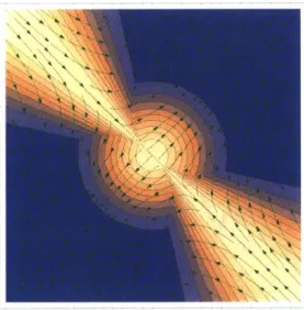
5-1 The density of !j(x; 1,1) + !K(x; -1,1). . . . . 95 5-2 Illustration of the Speed of Convergence of EM in Multiple Dimensions as

List of Tables

Chapter 1

Introduction

The field of optimization is concerned with solving the problem:

maxo(x)

XED

In this general version of the problem, without any restriction on the domain D and on V' it is very easy to show that this problem is very difficult to solve

[7].

This suggests that it is unavoidable to make some assumptions. A most helpful assumption that we can make is D to be a convex set and 0 to be a convex function. In this case the problem is called

convex optimization problem. There is a very long line of work investigating and analyzing

algorithms that solve convex optimization problems [9]. But in a lot of areas of science, the optimization problems that arise are not convex. This creates the area of non-convex

optimization. In contrast with convex optimization, there is no general theory and tools for

analyzing and finding theoretically proven algorithms for solving the non-convex problems. Actually, most of the techniques that we know are heuristic and sometimes we cannot even prove that they converge to local optima.

Non-convex optimization lies at the heart of some exciting recent developments in ma-chine learning, optimization, statistics and signal processing. Deep networks, Bayesian in-ference, matrix and tensor factorization and dynamical systems are some representative examples where non-convex methods constitute efficient - and, in many cases, even more ac-curate - alternatives to convex ones. However, unlike convex optimization, these non-convex

approaches often lack theoretical justification.

The above facts have triggered attempts in providing answers to when and why non-convex methods perform well in practice in the hope that it might provide a new algorithmic paradigm for designing faster and better algorithms.

A diverse set of approaches have been devised to solve non-convex problems in a variety of approaches. They range from simple local search approaches such as gradient descent and alternating minimization to more involved frameworks such as simulated annealing, continuation method, convex hierarchies, Bayesian optimization, branch and bound, and so on. Moreover, for solving special classes of non-convex problems there are efficient methods such as quasi convex optimization, star convex optimization, submodular optimization.

The goal of this master thesis is to prove the generality of a technique in analyzing the performance of iterative heuristic algorithms. This technique is based on the notion of

contraction maps and Banach's Fixed Point Theorem. We approach this proof of generality

both from a pure mathematical point of view and from a complexity theoretic point of view. In the second part of the thesis, inspired by the results of the previous part, we analyze a very well known heuristic algorithm for a non-convex problem, the EM algorithm. EM algorithm, is defined to solve a very important and generally non-convex problem, namely the maximum-likelihood maximization problem. We prove a positive result, analyzing EM for a paradigmatic case of finding the centers of a mixture of two Gaussians. This performance of EM even in this restricted case was an open problem since the definition of EM at 1977 [26].

1.1

Solution of a Non-Convex Optimization as a Fixed

Point and the Basic Iterative Method

Working on a domain D, the abstract goal of a huge class of algorithms is to find a point x* E D with some desired properties. In many cases these properties might be difficult to express. Sometimes even given a solution x* there is no obvious way to verify that this is actually a solution. A common way to overcome these difficulties, is to express the solutions as fixed points of an easily described function. More formally we can define a function

f

: D D such that the solution point x* E D satisfies f(x*) = x*. This way of expressing solutions is very common in a lot of scientific areas, e.g. equilibria in games [46], solutions of differential equations [14], a huge class of numerical methods [42].

Because of the importance of such a representation, a lot of interesting and important questions arise. Given a function

f

: D -+ D: is there any fixed point? is there a procedure that converges to this fixed point?

The first question, can be handled from important theorems in the field of topology called Fixed Point Theorems. Some of the most known once are : Brouwer's Fixed Point Theorem, Tikhonov's Fixed Point Theorem, Kakutani's Fixed Point Theorem and others [30].

The second question, while seemingly more difficult, has a very simple and intuitive can-didate solution. If

f

has a fixed point and under some regularity conditions, like continuity, we can define the following sequence of point

where the starting point x0 can be picked arbitrarily. If (xn) converges to a point fz then

lim Xn+1 = lim f(Xn) = lim Xn+1 =

f

limxn) -> z =

f(z)

n-+co n-4oo n-+oo (n-co

This observation means that a candidate procedure for computing such a fixed point is to iteratively apply the function

f

starting from an arbitrary point x0. If this procedure

converges we have the wanted fixed point x*.

So one last question that we have to answer is whether this sequence (Xn) actually con-verges. One of the most known techniques to prove that (xn) converges is to find a potential function 0. Usually a potential function, or Lyapunov function, is a lower bounded, real

valued function that decreases with every application of

f.

More formally

#

: D - R+ and

0(f(x)) < O(x). If we provide such a function and under some regularity conditions we can

make sure that the sequence (xn) converges and provides us with an algorithm that finds a fixed point of

f.

We will refer to this method of computing fixed points as the Basic Iterative Method.

1.1.1

An Algorithmic Point of View

The main performance guarantee of an algorithm is its running time. Therefore the first question that arises from a computer science perspective is: what is the running time of computing a fixed point and more specifically of the Basic Iterative Method?

We have seen that the potential function gives a general way of proving that the Basic Iterative Method converges. Moreover in the theory of dynamical systems there is a cele-brated result called Conley's Decomposition Theorem

[15].

One consequence of this work is that if a continuous analog of the Basic Iterative Method converges then there exist a potential function that can prove it. Therefore looking for potential functions in order to prove convergence does not restrict our power for proving convergence, because if there exists any argument to prove so there also exists a potential function argument.

But potential functions cannot tell us anything about the running time of the Basic Iterative Method. So one the main question that we would like to answer in this thesis is: is there a general way to upper and lower bound the running time of the Basic Iterative Method?

In the next sections we present our proposed direction for answering both the problems of lower and upper bounding the running time. Also in the last session we explain some important instantiations of the Basic Iterative Method that we don't know how to analyse and we hope we can get an answer after developing these general techniques.

1.2

Contraction Maps

-

Banach's Fixed Point Theorem

One of the main Fixed Point Theorems that we haven't mentioned yet is Banach's Fixed

Point Theorem

[5].

Informal Theorem (Banach's Fixed Point Theorem). If there is a distance metric function d, such that (D, d) is a complete metric space and f is a contraction map with contraction

constant c E (0,1) with respect to d, then f has a unique fixed point x* and the convergence rate of the Basic Iterative Method with respect to d is c'.

The last sentence in the statement of the theorem implies that after n iterations of the Basic Iterative Method the distance of x, from x* decreases by factor cn, i.e. d(xn, x*) <

c'd(xo, x*). There is a very nice algorithmic implication of this result. If we are only interested to find a point that is only E-close with respect to d to x* then the Basic Iterative

Method will finish after loge E steps.

This theorem therefore provides a way to prove all of: existence of fixed point, uniqueness of fixed point, convergence of Basic Iterative Method and most importantly bounds the running time of the Basic Iterative Method.

The applications of this theorem are very important and distributed in a lot different subjects. One of the most celebrated ones is to prove the existence of a unique solution to differential equations through Picard's Theorem and also for bounding the running time of numerical methods that solve these differential equations [14], [42].

But how general can this contraction map argument be? Is there a sort of converse theorem like there is for the potential function argument?

The answer for most of the implications of Banach's Fixed Point Theorem is yes! There are converses of Banach's Fixed Point Theorems which prove the following [8].

Informal Theorem (Bessaga's Converse Fixed Point Theorem). If

f

has a unique fixed point then for every constant c E (0,1) there exists a distance metric

function

d, such that (D, d,) is a complete metric space and f is a contraction map with contraction constant c with respect to d,.

The implication of this converse theorem is that if we want to prove existence and unique-ness of fixed points of

f

and convergence of the Basic Iterative Method then Banach's Fixed Point Theorem is the most general way to do it. This also proves that when we have only one fixed point x*, there exists a potential function of the form

#(x)

= dc(x, x*) where dc is a distance metric function that makes (D, d,) complete metric space.

But what are the actual implications for the complexity of computing a fixed point? The problem with the running time implications of the theorem, is that after loge E steps of the Basic Iterative Method we just have de(x,, x*) < E. But it is not clear what is the natural meaning of d,. It might not have any relation to the metric that we are interested in, i.e. the metric d for which we want a point x such that d(x, x*) E. So this Converse Theorem

running time of Basic Iterative method.

So our starting point instead of just the function

f

and the domain D should also be the complete distance metric function d that we are interested in. One step in this direction has

been done by Meyers

[441.

Informal Theorem (Meyers's Converse Fixed Point Theorem). If (D, d) is a complete

metric space, D is compact, f has a unique fixed point and the Basic Iterative Method converges then for any c E (0,1) there exists a distance metric function d, equivalent with d such that (D, d,) is a complete metric space and f is a contraction map according to d,.

The basic improvement in this theorem is that, instead of an arbitrary metric, it provides a metric equivalent with the metric that we started with. In order to do so Meyers's Converse Fixed Point Theorem has to assume that the Basic Iterative Method converges therefore we have to already have a proof of that in order to use it. Although this is a good step in the direction it is not enough in order to bound the number of steps needed by the Basic Iterative Method in order to get d(xn, x*) < F.

Our basic goal for this section is to close this gap under the assumptions of Meyers's Converse Fixed Points Theorem. The basic observation that we have is that in order for a fixed point x* to be stable there exists, usually, an open neighborhood of x* of radius 6 > 0 where

f

is a contraction according to d. This allows us to define d, = d around this neighborhood. For the rest of the space we extend d, in a way such that the contraction mapping condition is satisfied. This extension is inspired by the techniques that have been used for proving the mentioned Converse Fixed Point Theorems. After succeeding that we will have the guarantee that for any E < J the condition dc(xn, x*) e implies d(xn, x*) < e. This will let us prove the generality of Banach's Fixed Point Theorem for upper bounding the running time of the Basic Iterative Method in a statement like the following

Informal Theorem. Let (D, d) be a complete metric space and f : D -+ D be a self-made

that has a unique fixed point x* and every x converges to it. Then for any c E (0,1) there

exists a complete distance metric de, such that f is a contraction with constant c with respect to d,. Additionally, closeness of an arbitrary point x to x* with respect to d, implies closeness of x to x* with respect to d.

1.3

Computational Complexity of Fixed Points

Thus far we have discussed fixed point theorems, iterative methods, and the role of potential functions in establishing their convergence. We have also seen their interplay in Banach's fixed point theorem. In this section, we explore how the computational complexity of fixed points, potential function arguments and Banach's theorem are related. This question was one of the main motivations for a long line of research work starting with the papers of Johnson, Papadimitriou, Yannakakis [37] and Papadimitriou [481. These papers define re-spectively the complexity class PLS, capturing the complexity of computing local optima of a given potential function q, and the class PPAD, capturing the complexity of finding a fixed point of a continuous function

f.

Daskalakis and Papadimitriou [23] define the class CLS which relates to these classes as follows:

1. PLS

[37]:

when

#

satisfies some continuity condition

2. PPAD [481: when

f

satisfies some continuity condition

3. CLS

[23]:

when both

#

and f satisfy some continuity condition

A main problem that has been left open in the work of [23] is which of these classes captures the complexity of computing a fixed point whose existence is guaranteed by Banach's Fixed Point Theorem. We will refer to this problem as BANACH. More precisely in [23] they have shown that BANACH E CLS but it was left open whether BANACH is complete for

CLS.

Our main idea for solving this problem is to adjust the proofs of the Converse Fixed Point Theorems appropriately so that the procedure that constructs d, becomes computationally efficient. This would be a reduction that shows the completeness of BANACH for CLS. Obviously one bottleneck here is that Banach's Fixed Point Theorem guarantees the existence of a unique fixed point whereas general CLS allows multiple fixed points to exist. We were able to overcome this difficulty by accepting as solutions points that don't satisfy the contraction property. This way we can also have a nice correspondence between the promise class that promises the existence of only one fixed point and the promise class that BANACH defines and guarantees the validity of the contraction map condition.

1.4

Runtime Analysis of EM Algorithm

In the field of algorithms for inference one of the most important problems, is finding the hypothesis that maximizes the likelihood from a predefined set of hypotheses. The problem of directly maximizing such an objective might be too difficult. Even to verify the optimality of the solution is not a trivial problem in this case. The only obvious way to solve it might be the brute force algorithm.

In [26], the authors follow the direction that we described in the Introduction defining a function

f

whose set fixed points includes the solutions to the maximum likelihood problem. More precisely if x* is the hypothesis, from the set of hypothesis D, that maximizes the likelihood function then f(x*) = x*. This function

f

is called the EM Iteration and the Basic Iterative Method of the EM Iteration is called EM algorithm 1 2. Since then, the EM algorithm became the main tool for computing the solution to the maximum likelihood problem with very good practical guarantees and running times.

Despite its practical importance, too little is known theoretically about the convergence of the algorithm. For example it is known that when the likelihood is a unimodular function then the EM algorithm converges [57J. Under some other conditions the convergence of EM algorithm is also understood [59]. Although a little has been known about the convergence of the EM algorithm, only recently did some results appear about the running time of the EM algorithm. These results apply only to some restricted cases which are nevertheless the paradigmatic applications of the EM algorithm.

In this part of our work, we provide general unconditional guarantees about the perfor-mance of the EM algorithm based on the techniques and the intuition that we developed in the work described in the previous sections. This achievement would is a great step in analyzing algorithms that use the Basic Iterative Method. This kind of algorithms are very common in the area of Machine Learning and EM is a very important and paradigmatic

'The name EM comes from the fact that f is a back to back application of an Expectation and a

Maximization operators.

2

Notice that there are fixed points which do not correspond to maximum likelihood solutions. Nevertheless in a lot of important instantiations, the region of attraction of these dummy fixed points is limited, as it has been observed in practice. Therefore choosing only a few random starting points we can be almost sure that we have found the appropriate region of attraction.

one. This analysis of this case of the EM algorithm, we hope that will help in the theoretical analysis of other important algorithms in machine learning.

1.4.1

Mixture of Two Gaussians with Known Covariance Matrices

Let us assume that we are getting samples from a mixture of two Gaussians in n dimensions and we know their covariance matrices. We would like to recover the means of the two Gaussians, that is to find the hypothesis about the means that maximizes the likelihood function. This is a well studied problem and although there is a growing number of theoretical guarantees to solve this problem [17], [38], [21], [51], in practice the most useful technique is to run the EM algorithm. Although the model is very restricted and the EM iteration has a nice form in this case, still too little is known about the theoretical performance of EM algorithm in this case. Very recently Balakrishnan, Wainwright and Yu

[3j

and Yang, Balakrishnan and Wainwright [601 were the first to find a way to prove that there is an ball

B around the correct hypothesis x* such that if xO E B then the EM algorithm converges to the correct solution and also with very good convergence rate.

Based on the intuition we have from what we explained at Section 2, we find a way to analyze EM algorithm when applied to the mixture of two Gaussians case. This way we provide the first unconditional theoretical guarantees for EM applied to the mixture of two Gaussians.

Chapter 2

Notation and Preliminaries

We start this chapter by defining the notation that we will use for the rest of the thesis. Then we also give and explain the basic definitions that span the basic concepts of topological spaces, metric spaces, continuity and computational complexity theory. While giving these basic definitions we also state and prove some basic results of the literature that we are going to use later.

2.0.2

Basic Notation and Definitions

- R set of real numbers.

- R+ set of non-negative real numbers.

- R n n-dimensional Euclidean space.

- R"xf the space of real valued n x n matrices.

- AT the transpose of the real matrix A.

- N set of natural numbers.

- N1 set of natural numbers except 0.

- A \ B all the set A apart from the members that belong to B too.

- Ac the complement of the set A.

f [n] n times composition

f

with it self, i.e.

f... f

n times -

I

-1H1

- Int(S) -

Clos(S)

-

diamd

_[W] - B(x, r) -

B(x,

r)

-S*

fP norm of a vector in R". Mahalanobis distance norm.

set of equivalence classes of the equivalence relation - on a set D. interior of the set S.

closure of the set S.

diameter of the set W with respect to the distance metric d. open ball around x of diameter r.

closed ball around x of diameter r. Kleene star of a set S.

Table 2.1: Basic Notation

A real valued function g : D2 -+ R is called symmetric if g(x, y) = g(y, x) and anti-symmetric if g(X, y) = -g(y,

x).

2.1

Set Theoretic Definitions

For this section we assume the reader is familiar with the basic set theoretic definitions. Based on those we define the notion equivalence relation and equivalence classes and we

define and explain the Axiom of Choice.

2.1.1

Equivalence Relations

A relation R on a set X is a subset of X x X. An equivalence relation is a relation R that satisfies the following three properties

Reflexivity for all x E X, (x, x)

EE

R.

Symmetry for all x, y E X, (x, y) E R 4> (y, x) E R.

Transitivity for all x, y, z E X, (x, y) E R and (y, z) E R => (x, z) E R.

If ~ is an equivalence relation on X and x E X, the set Ex = {y

I

y E S and x ~ y} is called the equivalence class of x with respect to ~. The set of all the equivalence classes of

X for ~ is

X1 ={Ex I x C X}

2.1.2

Axiom of Choice

The importance of the Axiom of Choice to a huge range of pure mathematics can be indicated by the following sentence of an introduction to the Axiom of Choice from the Stanford Encyclopedia of Philosophy.

The principle of set theory known as the Axiom of Choice has been hailed as "probably the most interesting and, in spite of its late appearance, the most discussed axiom of mathematics, second only to Euclid's axiom of parallels which was introduced more than two thousand years ago".

Axiom of Choice. If A is a family of nonempty sets, then there is a function f with domain A such that f(a) E a for every a E A. Such a function f is called a choice function for A.

Axiom of Choice is known to be equivalent with a lot of very well known theorems, lemmas or principles. Some of them are: Zorn's Lemma, Well-ordering principle, Tychonoff's theorem and more. One such equivalent theorem is the Bessaga's theorem that we present, prove and explain in Chapter 3.

2.2

Topological and Metric Spaces

In this section we give the basic definitions and properties of topological and metric spaces that we are going to use in Chapter 3, when discussing about the converses of Banach's Fixed Point Theorem. Throughout this section we are working on a domain set D which is an arbitrary set. The material of this chapter is based on the notes by

[411.

2.2.1

Topological Spaces

We first give the definition of a topology and then based on this we define topological spaces.

Definition 1. Let E be a set and T a collection of subsets of E with the following properties. (a) The empty set 0 E r and the space D E r.

(b) If Ua

CTfor

all a E A then UaEAUa ET.

(c) If Uj G

-Ffor

all1 j nEN, then

nl>

Uj E T.

Then we say that T is a topology on D and that (X, T) is a topological space.

Example. If D is a set and T =

{0,

D}, then T is a topology. We call

{0,

D} the indiscrete topology on D. The reason of the name will become clear when we will define the discrete metric and its induced topology.

If (D, T) is a topological space we define the notion of open set by calling the members of T open sets. Now a subset C of D is called closed if E) \ C is an open set, i.e. belongs to T.

Definition 2. Let (D, T) and (X, T) be topological spaces. A function f : D -+ X is said to

be continuous if and only if f -1 (U) is open in D whenever U is open in Y.

Remark. We could start with closed sets the basic notion and then define topology, topo-logical spaces and continuity with respect to collections of closed sets, instead of open sets. The two types of definitions are completely equivalent and for historical reasons the definition based on open sets is the normal one.

2.2.2

Interior and Closure

Definition 3. Let (D, T) be a topological space and A a subset of D. We write

Int(A)=U{U

E T

I

U C

Al

(2.1)

Clos(a)

=

n{Uclosed I A C U}

(2.2)

and we call Clos(A) the closure of A and Int(A) the interior of A.

We now give some useful, basic lemmas without proof. A proof of those can be found in [41].

Lemma 1. (a) Int(A) = {x E A I 3U E T with x E U C A}.

(b) Int(A) is the unique V E T such that V C A and if W E T and V C W C A, then V = W. In other words, Int(A) is the largest open set contained in A.

Lemma 2. (a) Clos(A) = {x E Dj VU e 7with x E U, we have U n A # 0}.

(b) Clos(A) is the unique closed set V such that A C V and if W is closed and A C W C V,

then V = W. In other words, Clos(A) is the smallest closed set containing in A.

2.2.3

Metric Spaces

For the definition of metric spaces the most important is the definition of a distance metric

function.

Definition 4. Let D be a set and d: D2 _{-+ R a function with the following properties:}

(i) d(x, y) > 0 for all x, y E Domain. (ii) d(x, y) = 0 if and only if x = y.

(iii) d(x, y) = d(y, x) for all x, y E Domain.

(iv) d(x, y) <; d(x, z) + d(z, x) for all x, y, z E Domain. This is called triangle inequality. Then we say that d is a metric on D and (D, d) is a metric space.

Definition 5. The diameter of a set W C D according to the metric d is defined as

A metric space (D, d) is called bounded if diamd [D] is finite.

Definition 6. If D is a set and we define ds : E2 -+ R by

ds(x, y) 0 x=y

1 X # y

then ds is called the discrete metric on D.

Remark. It is very easy to see that discrete metric is indeed a metric, that is satisfies the conditions of Definition 4.

Now we can define the notion of continuity.

Definition 7. Let (D, d) and (X, d') be metric spaces. A function f : D -+ X is called continuous if, given x E D and E > 0, we can find a 6(x, e) such that

d'(f(x), f (y))

<

- whenever d(x, y) < 6(x, E)

Definition 8. Let (D, d) be a metric space. We say that a subset E C D is open in D if,

whenever e E E, we can find a 6 > 0 (depending on e) such that

x E E whenever d(x, e) < 6

The next lemma connects the definition of open sets according to some metric with the definition of open sets in a topological space.

Lemma 3. If (D, d) is a metric space, then the collection of open sets forms a topology.

Example. If (D, d) is a metric space with the discrete metric, show that the induced topology consists of all the subsets of D.

2.2.4

Closed Sets for Metric Spaces

Definition 9. Consider a sequence (xn) in a metric space (D, d). If x E D and, given E > 0,

we can find an integer N E N1 (depending maybe on e such that

d(xn,x) < Efor all n > N

then we say that x, -+ x as n -+ oc _{and that x is the limit of the sequence (xn).}

Remark. It is easy to see that if a sequence has a limit then this limit is unique.

Definition 10. Let (D, d) be a metric space. A set G C D is said to be closed if, whenever

xn E G and x,, -+ x then x E G.

Now that we have the notion of convergence of a sequence we can give the definition of compactness.

Lemma 4. Let (D, d) be a metric space and A a subset of D. Then Clos(A) consists of all

those x E D such that we can find (xn) with xnE A with d(xn, x) + 0.

Definition 11. A subset G of a metric space (D, d) is called compact if G is closed and

every sequence in G has a convergent subsequence.

A metric space (D, d) is called compact if D is compact and locally compact if for any

x E D, x has a neighborhood that is compact.

We define the closed ball of radius r around x to be B(x, r) = {y E D Id(x, y) < r}. One of the most important and exiting applications of the definitions of metric spaces and continuity is the following fixed point theorem by Brouwer.

Theorem 1. Let S C Rn be convex and compact. If T : S -+ S is continuous, then there

2.2.5

Complete Metric Spaces

We present the notion of complete metric spaces starting from the definition Cauchy se-quences.

Definition 12. If (D, d) is a metric space, we say that a sequence (xn) in D is Cauchy

sequence (or d- Cauchy sequence if the distance metric is not clear from the context) if, given

E > 0, we can find N(E)

E

N1 with

d(xn, xm) < E whenever nm > N(E)

Definition 13. A metric space (D, d) is complete if every Cauchy sequence converges. Definition 14. Two metrics d, d' of the same set D are called topologically equivalent (or

just equivalent) if for every sequence (x,) in D, (xn) is d-Cauchy sequence if and only if it is d'-Cauchy sequence.

2.2.6

Lipschitz Continuity

Definition 15. Let (D, d) and (X, d') be metric spaces. A function f : D --+ X is Lipschitz

continuous (or d-Lipschitz continuous if the distance metric is not clear from the context) if there exists a positive constant A E R+ such that for all x, y E D

d'(f(x),

f(y))

Ad(x, y)

Lemma 5. If a function f : D - X is Lipschitz continuous then it is continuous.

Definition 16. Let (D, d) and (X, d') be metric spaces. A function f : D - X is contraction (or d-contraction if the distance metric is not clear from the context) if there exists a positive constant 1 > c E R+ such that for all x, y C D

d'(f(x),

f(y))

< cd(x, y)

Definition 17. Let (D, d) and (X, d') be metric spaces. A function f : D - X is non-expansion (or d-non-non-expansion if the distance metric is not clear from the context) if for all

x,y E D

d'(f(x),

f(y))

<; d(x, y)

Definition 18. Let (D, d) and (X, d') be metric spaces. A

function

f : D -+ X is a similarity (or a d-similarity if the distance metric is not clear from the context) if there exists a positive constant 1 > c E R+ such that for all x, y E D

Chapter 3

Converse Banach Fixed Point Theorems

In this chapter we state prove and analyze the existing inverses of the Banach's Fixed Point Theorems. We focus on the applications of these theorems on the analysis of the running time of the Basic Iterative Method. Finally we prove an inverse theorem that has richer meaning from an algorithmic point of view.

For this chapter we will assume that the domain D admits a topology r according to which the function

f

: D D is continuous.

3.1

Banach's Fixed Point Theorem

Before presenting the inverses we state and prove the original Banach Fixed Point Theorem. The following presentation and proofs follow [16].

Theorem 2 (Banach's Fixed Point Theorem). If there is a distance metric

function

d, such

that (D, d) is a complete metric space and f is a contraction map according to d, i. e.

d(f(x), f(y)) c - d(x, y) with c < 1 (3.1)

then f has a unique fixed point x* and the convergence rate of the Basic Iterative Method with respect to d is c'.

Proof. First lets assume that there exist two different fixed points, x1, x2. Then by (3.1) we

have

which gives a contradiction.

Now we let x, be the sequence produced by the Basic Iterative Method on

f

starting from x0. We have that

d(x,,, x,,-)

c

-

d(x, ,Xfl2) < C2 -d(X,, 2, Xn-3) - <. n c

d(xi, xo)

Therefore the distance between x, and Xn- decreases an n increases. Using this property we can prove that (xn) is a Cauchy sequence.

Let N > n we get by triangle inequality

d(xN, Xn) d(xN, xN-1)-

+

d(Xn+ n(3.2)

< cNd(x₁,

x

0) + cN-ld(x1,

xo)

+... + C&d(x1,

x0)

(3.3)

< _

d(xi, xo)

(3.4)

1 - C

Therefore for any E > 0 we can pick M such that cM/(1 - c) < E and then the Cauchy

property holds for any n, N > M. Since (xn) is a Cauchy sequence we and the D is complete we have that (xn) converges. Let x* be the limit of (xn), that is x* = limna,0 Xn.

Now from the previous chapter we know that 5 every Lipschitz continuous function is also continuous. Therefore

f

is continuous by (3.1). So

Xn+1= f(xn) => lim Xn+1 =

f

( lim xn) = x' = f (x*)

n4oo n-+co

Therefore x* is the unique fixed point of

f

and the Basic Iterative Method converges to this fixed point.

One interesting generalization of Banach's Fixed Point theorem is one given by Edelstein [28]. This generalization will become useful to get some counter examples later when we present the Converse Theorems. Also the techniques used in the proof are very useful for the rest of this thesis.

Theorem 3. Let (D, d) be a compact metric space. If f : D -+ D satisfies

d(f(x), f(y)) < d(x, y) for x # y E D

then

f

has a unique

fixed

point in

D

and the fixed point can be

found

as the limit of f [nI(xo)

as n -4 oc for any x₀ E D.

Proof. To show

f

has at most one fixed point in D, suppose

f

has two fixed points a

#

b. Then d(a, b) = d(f(a),

f(b))

< d(a, b). This is impossible, so a = b.

To prove that

f

has actually a fixed point, we will look at the function D --+ [0, oc) given by x - d(x, f(x). This measures the distance between each point and its f-value. A fixed point of

f

is where this function takes the value zero.

Since D is compact, the function d(x, f(x)) takes in D its minimum value: there is an

a E D such that d(a, f(a)) < d(x, f(x)) for all x E D. We will show by contradiction that a

is a fixed point for

f.

If f(a)

#

a then the hypothesis about

f

in the theorem says

d(f(a),

f(f(a)))

< d(a,

f(a))

which contradicts the minimality of d(a, f(a)) among all numbers d(x, f(x)). So f(a) = a.

Finally, we show for any xo E D that the sequence xn = f[n] (x0) converges to a as n -+ oc.

This can't be done as in the proof of the Banach's Fixed Point Theorem since we don't have the contraction constant to help us out. Instead we will exploit compactness.

If for some k > 0 we have Xk = 1 then Xk+1 = f(Xk) = f(a) = a, and more generally

Xn = a for all n > k, so X -+ a since the terms of the sequence equal a for all large n. Now

we may assume instead that x,

#

a for all n. Then

0 < d(xn+l, a)

=

d(f(xn),

f(a))

< d(x,, a),

so the sequence of numbers d(xn, a) is decreasing and positive. Thus it has a limit f = limn, d(xn, a) > 0. We will show f = 0. By compactness of X, the sequence {xn} has a convergent subsequence xni, say xni -+ y E D. The function

f

is continuous, so

d(xa₁, a) -+ f and d(xn1

+i,

a) -+ f as i -+ oo. Since the metric, d(x, a) -+ d(y, a) and

d(xn1 1

,

a) = d(f(Xni), a) -+ d(f(y), a). Having already shown these limits are f,

d(y, a)

=

f

=

d(f(y), a)

=

d(f(y),

f(a))

If y = a the d(f(y),

f(a))

< d(y, a), but this contradicts the previous equation. So y = a,

which means f = d(y, a) = 0. That shows d(xn, a) -+ 0 as n -+ oc. l

3.2

Bessaga's Converse Fixed Point Theorem

In this section we give the first result that tries to capture the generality of the Banach's Fixed Point Theorem. This result is due to Bessaga [8] and was first published in 1959. There are at least four different proofs of this result. The first one, due to Bessaga

181,

uses a special form of the Axiom of Choice. This original version is not long, however, some statements are left to the reader for verifying.

The second proof, from Deimling's book [25] is a special case of that given by Wong

[56],

and it uses the Kuratowski-Zorn Lemma. In fact, Wong extended Bessaga's theorem to a finite family of commuting maps.

The third proof, due to Janos

1361,

is based on combinatorial techniques with a use of Ramsey's theorem. Actually, the existence of a separable metric is shown here (under the assumption that D has at most continuum many elements), though this metric need not be complete.

The last one, to the best of our knowledge, is due to Jachymski

[35]

and provides a nice direct connection with the existence of a potential function that decreases sufficiently at every step. Also, this proof enables us to get rid of the use of the Axiom of Choice when the metric space D is bounded and provides conditions under which

f

is a similarity.

We first state and prove a simple version of the theorem and we provide the first proof given by Bessaga in a simplified way. Then, we present the proof given by Jachymski and comment on the connection with the existence of a potential function. Finally we focus on the bounded case and the proof that is independent of the Axiom of Choice.

3.2.1

First Statement of Bassaga's Theorem

Formally, in the paper f81 Bessaga proved the following.

Theorem 4 (Bessaga's Converse Fixed Point Theorem). Let D

#

0 be an arbitrary set, f : D - D and c E (0,1). Then, if for all n E N, f [n] has a unique fixed point x* E D, then

there is a complete metric d for D such that d(f (x), f (y)) < c - d(x, y) for all x, y E D.

This proof of Bessaga's theorem is the one found on the blog "Bubbles Bad; Ripples Good", in an article with title "Bessaga's converse to the contraction mapping theorem" by

Willie Wong.

Proof. First we define an equivalence relation on D. We say x - y if there exists positive

integers p, q E N such that f[p](x) = f[q](y). If x ~ y we define

p(x, y) = min{p + q

I

f " (x) = f q] (y)} and

((x, y) = f(P)(x) where p is the value that attains p(x, y) We also define

O-(x, y) = p(x, (x, y)) - p(y, (x, y))

It is easy to prove that p is symmetric and o- antisymmetric.

Now, by the axiom of choice, there exists a choice function that chooses for each equiv-alence class of D/ - a representative, this extends to a function h : D -+ D by setting the

same value to all the members of the same equivalence class. We can now define a function

A: X -+ Z by

A(x) = u(h(x),x)

We are now in a position to define our distance function d. Let K = 1/c.

If x ~ y, we define

If x

6

x*, we define

d(x, x*) = K-(x)

If x 96 y and neither x, y is x*, we define

d(x, y)

=

d(x, x*) + d(y, x*)

By the definition of d we can see that it is symmetric and non-negative. It is also easy to check that d(x, y) = 0 ==> x ~ y and x = y = (x, y).

Triangle inequality involves a little bit more work, but most cases are immediately obvious except when x ~ y ~ z. Here we need to check that

K - K-\(Y)

-

K -K-A(xY))

-

K -K-A('(Yz)) > -K -K-A((x,z))

Suppose f [P(x) = f[qlj(y) and f[q21(y) = f[r](z). Without loss of generality we can take qi q2. Then we have that f [P](x) = f[r+1-q2](z). This shows that A( (x,z)) <

min(A( (x, y)), A( (y, z))). And this proves the inequality above.

Finally it is easy to see that any Cauchy sequence either is eventually constant, or must converge to x* : if x

76

y we have that

1

d(x, y) >

2-min(A(x),A(y))-1 > -(d(x,

)

+ d(y, ())

4

and this shows that d is a complete metric. Now, it remains to verify that

f

is a con-traction. Noting that A(f(x)) = A(x) + 1 and (f(x),

f(y))

= (x, y) we see easily that

f

is

a contraction with Lipschitz constant 1/K = c. E

3.2.2

Correspondence with Potential Function and Applications

In this section we present the work of Jachymski on a more simple proof of the Bessaga's theorem that also provides a connection with the existence of a potential function that decreases by a constant factor after every iteration of

f.

We start with the definition of Schr6der functional inequality, that captures this behaviour of the potential function.

functional inequality for f : D D with constant c E (0,1) if,

#(f(x)) 5 c - (x)

(3.5)

The following lemma proves that the existence of a potential function

#

that satisfies the Schr6der functional inequality implies the existence of a complete metric d for which f is a contraction map.

Lemma 6. Let f D -+ D and c E (0, 1). The following statements are equivalent: z. there exists a complete metric d for D such that

d(f(x),

f(y))

< c -d(x, y) for all x, y E D

ii. there exists a function

#

: D -> R+ such that 0-1_{({0}) is a singleton and the Schrdder}

functional inequality (3.5) holds.

The forward direction of the lemma is easy to see and explain while gives a proof that a potential of the form O(x) = d(x, x*) always exists. The inverse direction is not that

simple and is surprising because the intuition suggests that a complete metric has much more structure than a simple potential function.

Proof. i. ==>. ii. By the Banach's Fixed Point Theorem f has a fixed point x* and we can easily see that the potential function O(x) = d(x, x*) satisfies the Schr6der functional

inequality (3.5).

ii. =- i. Define d by d(x, y) = O(x) +

#(y)

if x # y and d(x, x) = 0. It is easily seen that d is a metric for D and by (3.5)

f

is a contraction with respect to d. To see this we verify that the conditions of Definition 4 are satisfied.

(i). Since O(x) > 0 obviously d(x, y) > 0.

(ii). If x , y then at least one of them is not equal to x* =

#-1({0}),

let x = x*. Obviously

then

#(x)

> 0 and therefore d(x, y)

#

0. The case x = y is captured by the definition of d. (iii). Obvious by the definition.

(iv). Since

#(z)

> 0 we have

d(x, y) = O(x) + #(y)

<;

#(x) + 0(y) + 2 -O(z) = d(x, z) + d(z, y)

Finally we have to prove that the metric space (D, d) is complete. Let (x,) be a Cauchy sequence. We may assume that the set {x, : n E N} is infinite, otherwise (xn) contains a constant subsequence and then (xn). Then there is a subsequence (xk,) of distinct elements so that

d(Xkn, Xkm) =

#(xkn)

+#$(Xk.) for n

h

m

Now since (xv) is a Cauchy sequence we know that d(Xk,, Xkm) -4 0 as n goes to +o and

m remains to the same distance from n. Therefore since

#(-)

> 0 we also get that

#(Xkn)

-+ 0

as n goes to infinity. But by the assumption of ii. we have that O(z) = 0 only for a unique

z E D. Therefore d(Xk,, z) =

#(xk,)

which means that d(Xkn, z) -÷ 0 and so (x,) converges

to z. 0

The above lemma can be used in order to prove the Bessaga's theorem as stated before.

3.2.3

Necessary and Sufficient Conditions for Similarity

Given the conditions of the Bessaga's Theorem and that

f

is injective we can prove not only that f is a contraction with respect to some complete metric of D but also that it is a similarity.

Theorem 5. Let f : D -+ D and c E (0,1). The following statements are equivalent.

(a) f is injective and f has a unique periodic point,

(b) f is an c-similarity with respect to some complete metric d.

One interesting question is what happens when the function f does not have any fixed points. Surprisingly enough there is a version of Lemma 6 that captures the case where f has no fixed point which we present next. Obviously if a function has more that one fixed point then any contraction or similarity conditions are impossible. To see this assume that x*, x are fixed points of

f.

Then d(f(x*), f(x*)) = d(x*, x*) and so the Lipschitz constant of

f

cannot be anything less than one.