Reduction and Introducer Concepts in d-Dimensional Contexts

HAL Id: hal-01706404

https://hal.archives-ouvertes.fr/hal-01706404v2

Submitted on 1 Feb 2019

HAL is a multi-disciplinary open access

archive for the deposit and dissemination of

sci-entific research documents, whether they are

pub-lished or not. The documents may come from

L’archive ouverte pluridisciplinaire HAL, est

destinée au dépôt et à la diffusion de documents

scientifiques de niveau recherche, publiés ou non,

émanant des établissements d’enseignement et de

Reduction and Introducer Concepts in d-Dimensional

Contexts

Alexandre Bazin, Giacomo Kahn

To cite this version:

Alexandre Bazin, Giacomo Kahn. Reduction and Introducer Concepts in d-Dimensional Contexts.

In-ternational Conference on Formal Concept Analysis, Jun 2019, Francfort, Germany. �hal-01706404v2�

Reduction and Introducers in d-contexts

Alexandre Bazin

Giacomo Kahn

1

_{LORIA, Nancy, France}

_{LIFO, Orléans, France}

Abstract

Concept lattices are well-known conceptual structures that organise interesting patterns – the concepts – extracted from data. In some applications, the size of the lattice can be a problem, as it is often too large to be efficiently computed and too complex to be browsed. In others, redundant information produces noise that makes understanding the data difficult. In classical FCA, those two problems can be attenuated by, respectively, computing a substructure of the lattice – such as the AOC-poset – and reducing the context. These solutions have not been studied in d-dimensional contexts for d > 3. In this paper, we generalise the notions of AOC-poset and reduction to d-lattices, the structures that are obtained from multidimensional data in the same way that concept lattices are obtained from binary relations.

Introduction

Formal concept analysis (FCA) is a mathematical framework introduced in the 1980s that allows for the application of lattice theory to data analysis. While it is now widely used, its main drawback, scalability, remains. Many ways to improve it have been proposed over the years. Some focus on reducing the size of the dataset by grouping or removing attributes or objects while others prefer to consider only a substructure of the lattice.

The end result of two of those approaches – respectively reduced contexts and AOC-posets – are of interest in our work. The first is the state of the dataset in which no element can be considered redundant. The second is the substructure of the lat-tice composed of its elements that best describe each individual object or attribute. Both have been extensively studied in traditional, bidimensional FCA. However, such is not the case in Polyadic Concept Analysis (PCA), the multidimensional generaliza-tion of FCA. The nogeneraliza-tion of reducibility of polyadic contexts have only proposed in the 3-dimensional case [1] and, to the best of our knowledge, no work on introducer multidimensional concepts exist.

PCA gives rise to an even greater number of patterns and so scalability is even more of an issue. Additionally, we believe that introducer concepts can be of use to better

analyse d-dimensional data as each element is associated to multiple concepts instead of one. For these reasons, in this work, we define and study both the reducibility and the introducer d-ordered set of d-contexts.

The article is divided as follows: in the next section, Section 1, we give the nec-essary definitions and preliminaries in order to ensure a smooth reading of the paper. Section 2 is focused on dataset reduction while Section 3 introduces introducers. We conclude by highlighting some problems that may – or may not – be of interest in the future.

1

Formal and Polyadic Concept Analysis

1.1

Formal Concept Analysis

Formal Concept Analysis (FCA) is a mathematical framework that revolves around formal contextsas a condensed representation of lattices. This framework allows one to inject the powerful mathematical machinery of lattice theory into data analysis. FCA has been introduced in the 1980’s by a research team led by Rudolph Wille in Darm-stadt. It is based on previous work by Garrett Birkhoff on lattice theory [2] and by Marc Barbut and Bernard Monjardet [3].

In this section, we give the basic definitions of FCA. For an informative book, the reader can refer to [4]. From now on, we will freely alternate between notations ab and {ab} to denote the set {a, b}.

Definition 1. A (formal) context is a triple (O, A, R) where O and A are finite sets andR ⊆ O × A is a relation between them. We call O the set of (formal) objects and A the set of (formal) attributes.

A formal context naturally can be naturally represented as a cross table, as shown in Figure 1. A pair (o, a) ∈ R corresponds to a cross in cell (o, a) of the cross table. Such a pair is read “object o has attribute a”. Since many datasets can be represented as binary relation such as the one in Figure 1, FCA finds natural applications in data analysis. a1 a2 a3 a4 a5 o1 × × × o2 × × × o3 × × × o4 × × o5 × × × o6 × × × o7 × × × ×

Figure 1: An example context with O = {o1, o2, o3, o4, o5, o6, o7} and A =

{a1, a2, a3, a4, a5}. A cross in a cell (o, a) is read “object a has attribute a”. A

To allow one to efficiently jump from a set of objects to the set of attributes that describes it, and vice versa, two derivation operators are defined. For a set O of objects and a set A of attributes, they are defined as follows:

·0: 2O7→ 2A

O0 = {a ∈ A|∀o ∈ O, (o, a) ∈ R} and

·0: 2A7→ 2O

A0= {o ∈ O|∀a ∈ A, (o, a) ∈ R}.

The ·0 derivation operator maps a set of objects (resp. attributes) to the set of at-tributes (resp. objects) that they share. The composition of the two derivation opera-tors (·00) forms a Galois connection. As such, it forms a closure operator (an extensive, increasing and idempotent operator). Depending on which set the composition of op-erators is applied, we can have two closure opop-erators : ·00: 2O 7→ 2O_{or ·}00_{: 2}A_{7→ 2}A_.

A set X such that X = X00is said to be closed.

Definition 2. A pair (O, A) where O ⊆ O and A ⊆ A are closed, A = O0 and O = A0is called aconcept. O is called the extent of the concept while A is called the intent of the concept.

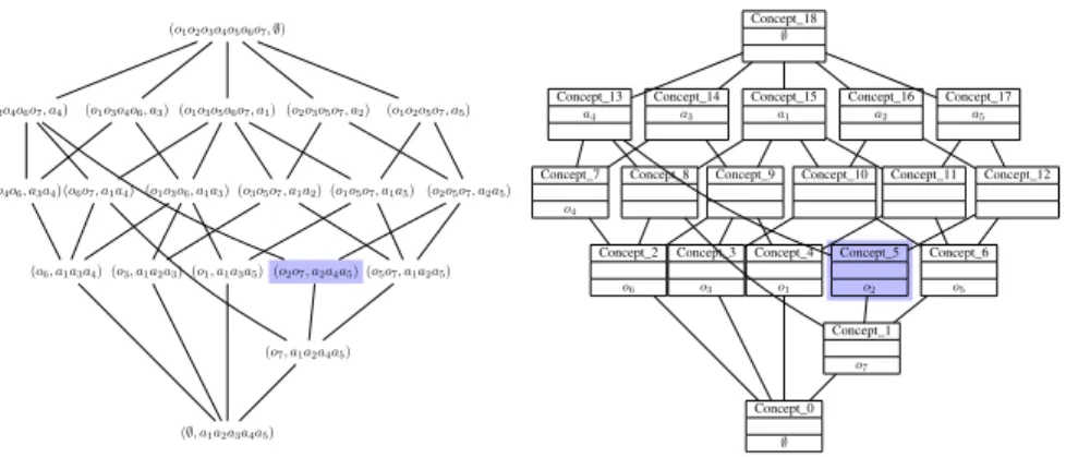
A concept corresponds to a maximal rectangle of crosses in the cross table that represents a context, up to permutation on rows and columns. In Figure 1, the concept (o2o7, a2a4a5) is highlighted. We denote by T (C) the set of all concepts of a context

C. (∅, a1a2a3a4a5) (o7, a1a2a4a5) (o6, a1a3a4) (o3, a1a2a3) (o1, a1a3a5) (o2o7, a2a4a5) (o5o7, a1a2a5) (o4o6, a3a4)(o6o7, a1a4) (o1o3o6, a1a3) (o3o5o7, a1a2) (o1o5o7, a1a5) (o2o5o7, a2a5) (o2o4o6o7, a4) (o1o3o4o6, a3) (o1o3o5o6o7, a1) (o2o3o5o7, a2) (o1o2o5o7, a5) (o1o2o3o4o5o6o7, ∅) Concept_0 ∅ Concept_1 o7 Concept_2 o6 Concept_3 o3 Concept_4 o1 Concept_5 o2 Concept_6 o5 Concept_7 o4

Concept_8 Concept_9 Concept_10 Concept_11 Concept_12 Concept_13 a4 Concept_14 a3 Concept_15 a1 Concept_16 a2 Concept_17 a5 Concept_18 ∅

Figure 2: Concept lattice corresponding to the example in Figure 1 (left) and with simplified labels (right).

The concepts of T (C) can be ordered. Let (O1, A1) and (O2, A2) be concepts of

a context. We say that (O1, A1) is a subconcept of (O2, A2) (denoted (O1, A1) ≤

(O2, A2)) if O1 ⊆ O2. As the Galois connection that rises from the derivation is

antitone, this is equivalent to A2 ⊆ A1. The concept (O2, A2) is a superconcept of

The set of concepts from a context ordered by inclusion on the extents forms a complete lattice called the concept lattice of the context. Additionally, every complete lattice is the concept lattice of some context, as stated in the basic theorem of formal concept analysis [4]. Figure 2 (left) shows the concept lattice corresponding to the example in Figure 1. One can check that the concepts of Figure 2 (left) correspond to maximal boxes of incidence in Figure 1. The highlighted concept (o2o7, a2a4a5)

corresponds to the highlighted concept of Figure 1. The concepts that are located directly above (upper cover) and directly below (lower cover) a concept X form the conceptual neighbourhoodof X.

Two types of concepts can be emphasised.

Definition 3. Let o be an object of a formal context. Then, the concept (o00, o0) is called anobject-concept. It is also called the introducer of the object o.

Definition 4. Let a be an attribute of a formal context. Then, the concept (a0, a00) is called anattribute-concept. It is also called the introducer of the attribute a.

For example, in Figure 2, the emphasised concept corresponds to the concept (o002, o02), and it introduces o2 in the sense that it is the least concept that contains

o2. In [4], such concepts are denoted respectively ˜γo for object-concepts and ˜µa

for concepts. A concept can be both an object-concept and an attribute-concept. Concepts that are neither attribute-concepts nor object-concepts are called plain-concepts. Those concepts will be the main character in Section 3 of this article.

The simplified representation of a concept lattice is a representation where the la-bels of the concepts are limited, in order to avoid redundancy. The label for a particular object appears only in the smallest concept that contains it (its introducer). Reversely, the label for a particular attribute appears only in the greatest concept that contains it (its introducer). The other labels are inferred using the inheritance property. Figure 2 (right) corresponds to the concept lattice from Figure 2 (left), with simplified labels. The concept named Concept_10 has both labels empty. By applying the inheritance, we can retrieve that Concept_10 is in fact the concept (o3o5o7, a1a2).

This representation allows for a better reading into the concepts (with a clear sep-aration between the extent and the intent of a concept). It allows to see at first glance which concepts are objects-concepts and attribute-concepts (by definition, the intro-ducers have non-empty labels). The plain-concepts are, quite literally, plain.

1.2

Polyadic Concept Analysis

Polyadic Concept Analysis is a natural generalisation of FCA. It has been introduced firstly by Lehmann and Wille [5, 6] in the triadic case, and then generalised by Vout-sadakis [7].

It deals with d-ary relations between sets instead of binary ones. More formally, a d-context can be defined in the following way.

Definition 5. A d-context is a (d + 1)-tuple C = (S1, . . . , Sd, R) where the Si, i ∈

S1

S2

S3

Figure 3: Visual representation of a 3-context without its crosses.

A d-context can be represented as a |S1| × · · · × |Sd| cross table, as shown in

Figure 3. For technical reasons, most of our examples figures will be drawn in two or three dimensions.

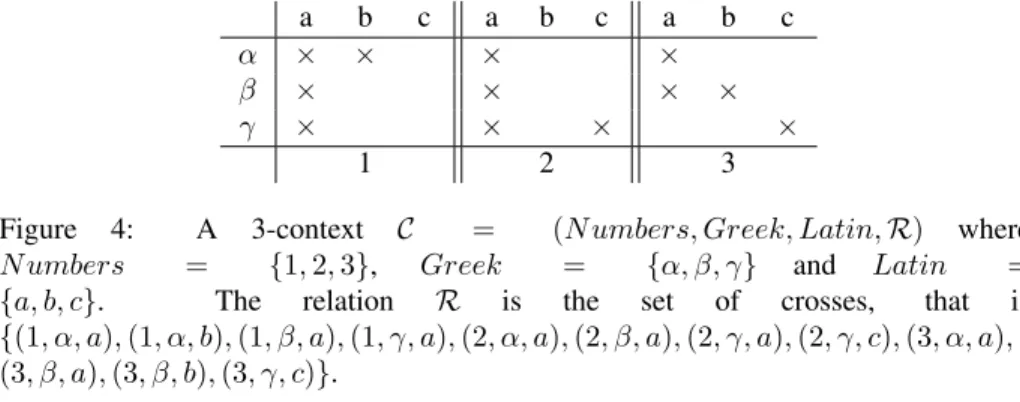
When needed, one can represent a d-context by separating the “slices” of the cross table. For instance, Figure 4 shows a 3-context which dimensions are N umbers, Latin, and Greek.

a b c a b c a b c

α × × × ×

β × × × ×

γ × × × ×

1 2 3

Figure 4: A 3-context C = (N umbers, Greek, Latin, R) where N umbers = {1, 2, 3}, Greek = {α, β, γ} and Latin = {a, b, c}. The relation R is the set of crosses, that is {(1, α, a), (1, α, b), (1, β, a), (1, γ, a), (2, α, a), (2, β, a), (2, γ, a), (2, γ, c), (3, α, a), (3, β, a), (3, β, b), (3, γ, c)}.

In the same way as in the 2 dimensional case, d-dimensional maximal boxes of incidence have an important role.

Definition 6. A d-concept of C = (S1, . . . , Sd, R) is a d-tuple (X1, . . . , Xd) such that

Q

i∈{1,...,d}Xi ⊆ R and, for all i ∈ {1, . . . , d}, there is no k ∈ Si\ Xi such that

{k} ×Q

j∈{1,...,d}\{i}Xj ⊆ R.

When the dimensionality is clear from the context, we will simply call d-concepts concepts.

Definition 7. Let_.i,i ∈ {1, . . . , d}, be quasi-orders on a set P . Then, P = (P, .1

1. A ∼iB, ∀i ∈ {1, . . . , d} implies A = B (Uniqueness Condition)

2. _{A .}i1 B, . . . , A .id−1 B implies B .idA (Antiordinal Dependency)

Let us now define d quasi-orders on a set of d-concepts of a d-context C: (A1, . . . , Ad) .i(B1, . . . , Bd) ⇔ Ai⊆ Bi

The resulting equivalence relation ∼i, i ∈ {1, . . . , d} is then:

(A1, . . . , An) ∼i(B1, . . . , Bn) ⇔ Ai= Bi

We can see that the set of concepts of a d-context, together with the quasi-orders and equivalence relations defined here, forms a d-ordered set. Additionally, the existence of some particular joins makes this d-ordered set a d-lattice. For a more detailed defi-nition, we refer the reader to Voutsadakis’ seminal paper on Polyadic Concept Analy-sis [7].

We can see that concept lattices are in fact 2-ordered sets that satisfy both the uniqueness condition and the antiordinal dependency.

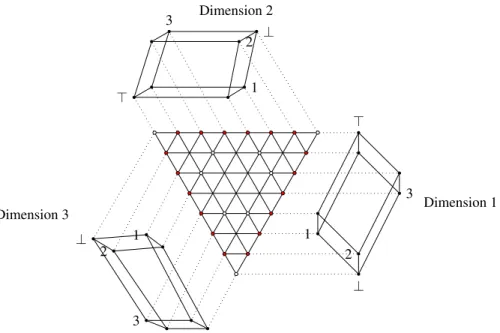
In order to fully understand d-lattices, let us illustrate the definition with a small digression about graphical representation. In 2 dimensions – i.e. concept lattices – the two orders (on the extent and on the intent) are dual and only one is usually men-tioned (the set of concepts ordered by inclusion on the extent, for example). Thus, their representation is possible with Hasse diagrams. From dimension 3 and up, the representation of d-ordered sets is harder. For example, in dimension 3, as of the time of writing, no good (in the sense that it allows to represent any 3-ordered set) graphical representation exists. However there is still a possible representation in the form of triadic diagrams.

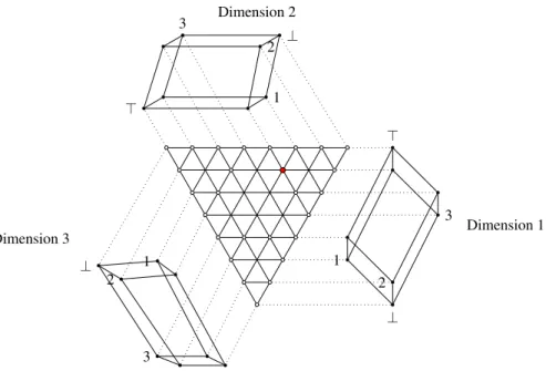
Figure 5 shows an example of a triadic diagram, a representation of a 3-ordered set. Let us explain how this diagram should be read. The white circles in the central triangle are the concepts. The lines of the triangle represent the equivalence relation between concepts: the horizontal lines represent ∼1, the north-west to south-east lines

represent ∼2and the south-west to north-east lines represent ∼3. Recall that two

con-cepts are equivalent with respect to ∼iif they have the same coordinate on dimension

i. This coordinate can be read by following the dotted line until the diagrams outside the triangle. In [5], Lehmann and Wille call the external diagrams the extent diagram, intent diagramand modi diagram depending on which dimension they represent. Here, to pursue the permutability of the dimensions further, we simply denote them by di-mension diagramfor dimension 1, 2 or 3.

If we position ourselves on the red concept of Figure 5, we can follow the dotted line up to the dimension 1 diagram and read its coordinate on the first dimension. It is {13}. Following the same logic for dimension 2 and 3, we can see that the red concept is (13, 12, 23). The concept on the south-east of the red concept is on the same equivalence line, with respect to ∼2. We know that its second dimension will be

{12} too. When we follow the lines to the other dimension diagrams, we see that it is (23, 12, 13).

Here, every dimension diagram is a powerset on 3 elements. It is not always the case, as the three dimension diagrams are not always isomorphic.

Dimension 1 Dimension 2 Dimension 3 > 3 1 2 ⊥ > 3 1 2 ⊥ ⊥ 2 1 3

Figure 5: Representation of a powerset 3-lattice. The red concept is (13, 13, 23).

We mentioned earlier that this representation does not allow to draw any 3-lattice (with straight lines). In [5], Lehmann and Wille explain this by saying that a violation of the so-called ‘Thomsen Conditions [8]’ and their ordinal generalisation [9] may appear in triadic contexts.1

2

Reduction in d-contexts

2.1

Reduction in 2-contexts

Two concept lattices from different contexts can be isomorphic. Reduction is a way of reaching a canonical context, the standard context, for any finite lattice. Reduction can be described as a two steps process. The first step of reduction in 2-dimension is the fusion of identical rows or columns (clarification).

Definition 8 (Reformulated from [4, Definition 23]). A context (S1, S2, R) is called

clarified if for any objects o1ando2inS1,o01= o02implies thato1 = o2and for any

attributesa1anda2inS2,a01= a02impliesa1= a2.

In [4, Definition 23], the authors use the Figure 6 example of a context that rep-resents the service offers of an office supplies business and the associated clarified context.

1_{I was unable to put my hands on those two books in order to learn more about that. If you have a copy,}

Furniture Computers Copy-machine Typewriters Specialised machines Consulting × × × × × Planning × × Installation × × × × × Instruction × × × × Training × Spare parts × × × × × Repairs × × × × × Service contracts × × × Furniture Computers Copy-machine and Typewriters Specialised machines Consulting, Installation,

Spare parts, repairs × × × ×

Planning × ×

Instruction × × ×

Training ×

Service contracts × ×

Figure 6: Context and clarified context (from [4])

Another possible action is the removal of attributes (resp. objects) that can be written as combination of other attributes (resp. objects). If a is an attribute and A is a set of attributes that does not contain a but have the same extent, then a is reducible. Full rows and full columns are always reducible.

In a lattice, an element x is ∨-irreducible if x = a ∨ b implies x = a or x = b with a and b two elements of the lattice. An element x is ∧-irreducible if x = a ∧ b implies x = a or x = b, with a and b two elements of the lattice.

Definition 9 (Reformulated from [4, Definition 24]). A context (S1, S2, R) is called

row reduced if every object-concept is ∨-irreducible and column reduced if every attribute-concept is∧-irreducible. A context that is both row reduced and column reduced isreduced.

This yields that for every finite lattice L, there is a unique (up to isomorphism) reduced context such that L is the concept lattice of this context. This context is called the standard context of L. This standard context can be obtained from any finite context by first clarifying the context and then deleting all the objects that can be represented as intersection of other objects and attributes that can be represented as intersection of other attributes.

2.2

Generalisation to d-dimensions

A first generalisation to 3-dimensional contexts was made in [1] by Rudolph, Sacarea and Troanca. Here, we generalise further to the d-dimensional case.

To define reduction in multidimensional contexts, we need to recall some defini-tions. The following notations are borrowed from [7]. A d-context gives rise to

nu-merous2_{k-contexts, with k ∈ {2, . . . , d}. Those k-contexts correspond to partitions}

π = (π1, . . . , πk) of {1, . . . , d} into k disjoint subsets. The k-context corresponding

to π is then Cπ = (Q i∈π1Si, . . . , Q i∈πkSi, R π ), where (s(1), . . . , s(k)) ∈ Rπif and only if (s1, . . . , sd) ∈ R with si∈ s(j)⇔ i ∈ πj. The contexts Cπare essentially the

context C flattened by merging dimensions with the Cartesian product.

In the following, we consider only binary partitions with a singleton on one side and all the other dimensions on the other. Let π = (i, {1, . . . , d} \ i) be such a partition of {1, . . . , d}. Then, from the context C = (S1, . . . , Sd, R) we obtain the dyadic

context Cπ _{= (S}

i,Q_{j∈{1,...,d}\{i}}Sj, Rπ) where (a, b) ∈ Rπ if and only if a ∈ Si

and b = b1× · · · × bd−1∈Q_{j∈{1,...,d}\i}Sjand (a, b1, . . . , bd−1) ∈ R.

We refer the reader to figures 4 and 7 for a graphical representation of this transfor-mation. Such a binary partition gives rise to the dyadic derivation operators X 7→ X(π) on the 2-context Cπ.

(1,a) (1,b) (1,c) (2,a) (2,b) (2,c) (3,a) (3,b) (3,c)

α × × × ×

β × × × ×

γ × × × ×

Figure 7: Let C be our context from Figure 4. Let π = ({Greek}, {N umber, Latin}). This figure represents the 2-context Cπ.

Let x be an element of a dimension i of a d-context C. Then we denote by Cxthe

(d − 1)-context Cx = (S1, . . . , Si−1, Si+1, . . . , Sd, Rx) with Rx= {(x1, . . . , xi−1,

xi+1, . . . , xd) | (x1, . . . , xi−1, x, xi+1, . . . , xd) ∈ R}.

We first define clarified d-contexts. Just as in the 2-dimensional case, our definition is equivalent to the fusion of identical (d − 1)-dimensional layers.

Definition 10. A d-context (S1, . . . , Sd, R) is called clarified if, for all i in {1, . . . , d}

and anyx1, x2inSi,x (π) 1 = x

(π)

2 impliesx1= x2, withπ = (i, {1, . . . , d} \ i).

As with the 2-dimensional case, we provide an example in Figure 8.

Definition 11. A clarified d-context C = (S1, . . . , Sd, R) is called i-reduced if every

object-concept fromC(π)_{, withπ = (i, {1, . . . , d} \ {i}), is ∨-irreducible. A d-context}

isreduced if it is i-reduced for all i in {1, . . . , d}.

The most important property of reduction in the two dimensional setting is that the lattice structure obtained from the concepts of a given context is isomorphic to the one of its reduced context. The following proposition proves that the same holds for our definition of reduction in d dimensions.

Proposition 12. Let C = (S1, . . . , Sd, R) be a d context. Let π be a binary partition

(i, {1, . . . , d} \ {i}). Let yibe an element ofSiandYibe a subset ofSisuch thatyiis

a b c a b c a b c α × × × × β × × × × × γ × × × × × 1 2 3 (α, 1) (α, 2) (α, 3) (β, 1) (β, 2) (β, 3) (γ, 1) (γ, 2) (γ, 3) a × × × × × b × × × × × c × × × ×

a and b c a and b c a and b c

α × ×

β × × × ×

γ × × ×

1 2 3

Figure 8: A 3-context C = (N umbers, Greek, Latin, R) (above) and the 2-context Cπ _{with π = (Latin, {Greek, N umbers}). We can see that a}(π) _{= b}(π) ₌

{(α, 1), (α, 2), (β, 2), (γ, 1), (γ, 3)}, which means that a and b can be aggregated into a new attribute “a and b”. Below, the corresponding clarified 3-context.

not inYiandy (π) i = Y (π) i . Then, T (C) ∼= T    S1, . . . , Si\ {yi}, . . . , Sd, R ∩  Si\ {yi} × Y j∈{1,...,d}\{i} Sj      .

Proof. Without loss of generality, let us assume that yiis an element of S1. We have to

ensure that if (X1, . . . , Xd) is a concept of C, then (X1\ {yi}, . . . , Xd) is a concept in

the reduced context. In C, (X1\ {yi}, . . . , Xd) is a d-dimensional box full of crosses.

We have to show that removing yifrom X1does not allow it to be extended on any

other dimension. As (X1, . . . , Xd) is a d-concept, its components Xj, j 6= i form a

(d − 1)-concept in the intersection of all the layers induced by the elements of Xi.

As C is not reduced because of yi, Cyi is the intersection of at least two layers Ca

and Cb. Obviously, a and b are elements of X1. If (X2, . . . , Xd) is not a (d −

1)-concept in the intersection of the layers Cx, x ∈ X1\ {yi}, then it can be extended

using crosses that both Ca and Cb share. This means that Cyi should have them too,

preventing (S1, . . . , Sd, R) from being a concept in the first place. This ensures that

(X1\ {yi}, . . . , Xd) is indeed a concept.

This proposition states that removing a reducible element from a d-context does not change the structure of the underlying d-lattice. If we keep track of the reduced and clarified elements during the process, it is possible not to lose information (by creating aggregate attributes or objects for example). It is still a deletion from the dataset. In the next section we speak about introducer concepts in a multidimensional setting.

3

Introducer concepts

3.1

Introducer d-concepts

Reduction induces a loss of information in a dataset since reducible elements are erased. Lots of applications cannot afford this loss of information and have to use other ways of reducing the complexity. Another structure, smaller than the concept lattice, has been introduced by Godin and Mili [10] in 1993. This structure consists in the restriction of the lattice to the set of introducer concepts. In the general case, the properties that make a concept lattice a lattice are lost and we are left with a simple poset. Since dyadic FCA deals with objects and attributes, such a poset is also called an Attribute-Object-Concept poset, or AOC-poset for short. In this section, we introduce the introducer concepts in a d-dimensional setting.

Due to the unicity of the dyadic closure (one component of a concept leaves only one choice for the other), each element of a dimension has only one introducer. This bounds the size of an AOC-poset by the number of objects plus the number of at-tributes of a context, when a concept lattice can have an exponential number of objects or attributes. As we will see in the following, this property is lost when we go multidi-mensional.

Definition 13. Let i be a dimension called the height while all other dimensions are called the width. Letx be an element of dimension i. The concepts with maximal width such thatx is in the height are the introducer concepts of x.

a b c a b c a b c a b c

α × × × × × ×

β × × × × × ×

γ × × × × × × ×

1 2 3 4

Figure 9: This 3-context shall serve as an example of our definitions.

Let us consider the 3-context from Figure 9 as an example. The set of introducers of element a, denoted Ia is Ia = {(12, αβγ, a), (123, αβ, a), (1234, α, a)}. For the

element 3, we have I3= {(123, αβ, a), (3, β, ab), (34, βγ, b), (34, γ, bc)}.

We denote by I(Si) the union of the introducer concepts of all the elements of a

dimension i and by I(C) the set of all the introducer concepts of a context C. Proposition 14. (I(C),_.1, . . . , .d) is a d-ordered set.

Proof. Let A = (A1, . . . , Ad) and B = (B1, . . . , Bd) be elements of I(C). We recall

that Ai ⊆ Bi⇔ A .i B and that Ai = Bi ⇔ A ∼i B. Without loss of generality, A

is an introducer for an element of dimension i and B for an element of dimension j. If, for all k between 1 and d, A ∼k B, then for all k, Ak = Bk and A = B (Uniqueness

Condition).

Let us suppose that A and B are such that A_.i B, ∀i ∈ {1, . . . , d} \ {k}. Then,

necessarily, Bk ⊆ Ak or A would not be a d-concept. Hence, B .k A (Antiordinal

From now on we can mirror the terminology of the 2-dimensional case, where we have complete lattices and attribute-objects-concepts partially ordered set, and use complete d-lattices and introducers d-ordered sets.

The following proposition links introducer d-concepts with the (d − 1)-concepts that arise on a layer of a d-context.

Proposition 15. Let x be an element of Si. If (X1, . . . , Xi−1, Xi+1, . . . , Xd) is a

(d − 1)-concept of Cx, then there exists someXisuch that(X1, . . . , {x} ∪ Xi, . . . , Xd)

is an introducer ofx. If (X1, . . . , {x} ∪ Xi, . . . , Xd) is an introducer of x, then there

exists a(d − 1)-concept (X1, . . . , Xi−1, Xi+1, . . . , Xd) in Cx.

Proof. We suppose, without loss of generality, that x is in S1. The (d − 1)-concepts

of Cxare of the form (X2, . . . , Xd). If (x, X2, . . . , Xd) is a d-concept of C, then it is

maximal in width and has x in its height, so it is an introducer of x.

If (x, X2, . . . , Xd) is not a d-concept of C, it means that it can be augmented only

on the first dimension (since (X2, . . . , Xd) is maximal in Cx). Thus, there exists a

d-concept ({x} ∪ X1, X2, . . . , Xd) that is maximal in width and has x in its height and

is, as such, an introducer for x.

Suppose that there is a X = (X1, . . . , Xd) that is an introducer of x but that is not

obtained from a (d − 1)-concept of Cxby extending X1. It means that (X2, . . . , Xd) is

not maximal in Cx(or else it would be a (d−1)-concept). Then there exists a d-concept

Y = (Y1, Y2, . . . , Yd) with x ∈ Y1⊆ X1and Xi⊆ Yifor all i between 1 and d. This

is in contradiction with the fact that X is an introducer of x.

Proposition 15 states that every (d − 1)-concept of a layer Cxmaps to an introducer

of x in C and that every introducer of x is the image of a (d − 1)-concept of Cx. This

proposition results in a naive algorithm to compute the set of introducer concepts of a d-context. It is sufficient to compute the (d − 1)-concepts of the (d − 1)-contexts obtained by fixing an element of a dimension.

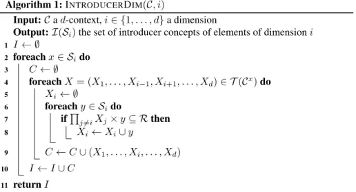
Algorithm 1 computes the introducers for each element of a dimension i. For a given element x ∈ Si, we compute T (Cx). Then, for each (d−1)-concept X ∈ T (Cx),

we build the set Xi needed to extend X into a d-concept. An element y is added to

Xiwhen y ×Qj6=iXj ⊆ R, that is if there exists a (d − 1)-dimensional box full of

crosses (but not necessarily maximal) in R, at level y. The final set Xialways contains

at least x. To compute the set introducer concepts for a d-context, one needs to call Algorithm 1 on each dimension of a d-context. In some applications, it may be useful to compute the introducer concepts with respect to a given quasi-order_.i.

3.2

Combinatorial Intuition : powerset d-lattices

Unlike the 2-dimensional case, where introducers are unique and the size of the AOC-poset is thus bounded by |S1| + |S2|, in the general case, it is bounded by Kd−1×

P

i∈{1,...,d}|Si|, with Kd the maximal number of d-concepts in a d-context. Since a

1-context has only one 1-concept, this bound is reached in the 2-dimensional case. Let us consider a powerset 3-lattice T(5) on a ground set of size 5. It is well known3 _{that T(5) has 3}5

= 243 concepts. However, the size of the introducer set of

Algorithm 1: INTRODUCERDIM(C, i)

Input: C a d-context, i ∈ {1, . . . , d} a dimension

Output: I(Si) the set of introducer concepts of elements of dimension i 1 I ← ∅

2 foreach x ∈ Sido 3 C ← ∅

4 foreach X = (X1, . . . , Xi−1, Xi+1, . . . , Xd) ∈ T (Cx) do 5 Xi ← ∅ 6 foreach y ∈ Sido 7 ifQ_j6=iX_j× y ⊆ R then 8 Xi ← Xi∪ y 9 C ← C ∪ (X1, . . . , Xi, . . . , Xd) 10 I ← I ∪ C 11 return I

the powerset trilattice T(5) is 30. Indeed, by Proposition 15 we know that there exists a mapping between the 2-concepts of each layer induced by fixing an element of a dimension and the introducers. As, by definition, every layer of the context inducing a powerset trilattice has two 2-concepts, the number of introducer concepts in a powerset 3-lattice on a ground set of five elements is then bounded by 3 × 5 × 2. This number is reached as the unique “hole” in each layer intersects all the concepts of the other layers. A more formal proof is given for a more general proposition below (Proposition 16).

In fact, for any powerset 3-lattice on a ground set of size n, the corresponding introducer d-ordered set has 3×2×n elements. Figure 10 shows a 4-adic contranominal scale on three elements. Figure 11 shows the introducers of the powerset 3-lattice on a ground set of 3 elements.

a b c a b c a b c A α × × × × × × × × β × × × × × × × × × γ × × × × × × × × × B α × × × × × × × × × β × × × × × × × × γ × × × × × × × × × C α × × × × × × × × × β × × × × × × × × × γ × × × × × × × × 1 2 3

Figure 10: This is a 4-adic contranominal scale where the empty cells have been framed. Every layer induced by fixing an element (for example A) has three 3-concepts (in CAwe have (123, αβγ, bc), (123, βγ, abc) and (23, αβγ, abc)).

Dimension 1 Dimension 2 Dimension 3 > 3 1 2 ⊥ > 3 1 2 ⊥ ⊥ 2 1 3

Figure 11: This represents a powerset 3-lattice. Its introducer concepts are filled in red.

Proposition 16. Let d be an integer. A powerset d-lattice Td_{(n) on a ground set of n}

elements hasdn_{elements. Its corresponding introducerd-ordered set has d×(d−1)×n}

elements.

Proof. Let C be a d-dimensional contranominal scale, that gives rise to Td_{(n). Let x}

be an element of a dimension. The (d − 1)-context Cxhas only one hole (by definition

of a contranominal scale). This implies that each (d − 1)-layer induced by fixing an element of a dimension has d−1 concepts. By Proposition 15, we know that there exists a mapping between the (d − 1)-concepts of the layers and the introducer concepts of the context. Since we have d dimensions and n layers by dimension, the number of introducer concepts is bounded by d × (d − 1) × n.

Moreover, let X = (X1, . . . , Xd) be an introducer concept for element x of

dimen-sion i. Then Xi = x. Indeed, by definition of a contranominal scale, there will be a

‘hole’ per layer of the context C that will be in the width of X.

This ensures that the d × (d − 1) × n introducer concepts that arise from Proposi-tion 15 are distinct and that this number is reached in the case of powerset d-lattices.

4

Open problems

With respect to reduction, it would be interesting to investigate the relation of irre-ducible elements to the Dedekind-MacNeille completion of d-ordered sets presented by Voutsadakis [12].

Some interesting questions remain open regarding the number of introducer con-cepts compared to the number of concon-cepts, both experimentally and theoretically. Fur-thermore, it would be interesting to use introducer concepts in visualisation or ex-plainable approaches in d-dimensions, as they give insight on the less general concepts containing an element.

References

[1] Sebastian Rudolph, Christian Sacarea, and Diana Troanca. Reduction in triadic data sets. In Proceedings of the 4th International Workshop "What can FCA do for Artificial Intelligence?", FCA4AI 2015, co-located with the International Joint Conference on Artificial Intelligence (IJCAI 2015), Buenos Aires, Argentina, July 25, 2015., pages 55–62, 2015.

[2] Garrett Birkhoff. Lattice theory, volume 25. American Mathematical Soc., 1940. [3] Marc Barbut and Bernard Monjardet. Ordre et classification. Algebre et

Combi-natoire, Volumes 1 and 2, 1970.

[4] Bernhard Ganter and Rudolf Wille. Formal concept analysis - mathematical foun-dations. Springer, 1999.

[5] Fritz Lehmann and Rudolf Wille. A triadic approach to formal concept analysis. In Conceptual Structures: Applications, Implementation and Theory, Third Inter-national Conference on Conceptual Structures, ICCS ’95, Santa Cruz, California, USA, August 14-18, 1995, Proceedings, pages 32–43, 1995.

[6] Rudolf Wille. The basic theorem of triadic concept analysis. Order, 12(2):149– 158, 1995.

[7] George Voutsadakis. Polyadic concept analysis. Order, 19(3):295–304, 2002. [8] David H. Krantz, Patrick Suppes, and Robert Duncan Luce. Foundations of

mea-surement. academic press, 1971.

[9] Utta Wille. Geometric representation of ordinal contexts. PhD thesis, University Gießen, 1995.

[10] Robert Godin and Hafedh Mili. Building and Maintaining Analysis-Level Class Hierarchies Using Galois Lattices. In 8th Conference on Object-Oriented Pro-gramming Systems, Languages, and Applications (OOPSLA), pages 394–410, 1993.

[11] Klaus Biedermann. Powerset trilattices. In Conceptual Structures: Theory, Tools and Applications, 6th International Conference on Conceptual Structures, ICCS ’98, Montpellier, France, August 10-12, 1998, Proceedings, pages 209–224, 1998.

[12] George Voutsadakis. Dedekind-macneille completion of n-ordered sets. Order, 24(1):15–29, 2007.