Automating comprehensive literature review of cancer risk journal articles

Automating Comprehensive Literature Review of

Cancer Risk Journal Articles

by

Heeyoon Kim

Submitted to the Department of Electrical Engineering and Computer

Science

in partial fulfillment of the requirements for the degree of

Masters of Engineering in Computer Science and Engineering

at the

MASSACHUSETTS INSTITUTE OF TECHNOLOGY

September 2017

c

○ Massachusetts Institute of Technology 2017. All rights reserved.

Author . . . .

Department of Electrical Engineering and Computer Science

August 18, 2017

Certified by . . . .

Regina Barzilay

Professor

Thesis Supervisor

Accepted by . . . .

Christopher J. Terman

Chairman, Masters of Engineering Thesis Committee

Automating Comprehensive Literature Review of Cancer Risk

Journal Articles

by

Heeyoon Kim

Submitted to the Department of Electrical Engineering and Computer Science on August 18, 2017, in partial fulfillment of the

requirements for the degree of

Masters of Engineering in Computer Science and Engineering

Abstract

Recently, researchers at the Massachusetts General Hospital and the Dana Farber Cancer Institute built a calculator that estimates risk of cancer based on genetic mutations. The calculator requires a lot of high quality data from medical journals, which is laborious to obtain by hand. In this thesis, I automate the process of obtaining medical abstracts from PubMed and develop a classifier that uses domain knowledge to determine relevant abstracts. The classifier is very accurate (percent correct = 0.898, F1 = 0.86, recall = 0.905), and is significantly better than the majority baseline. I explore an alternative model that exploits rationales within abstracts, which could lead to an even greater accuracy. After determining relevant abstracts, it’s useful to find the size of the cohorts, which is an indicator for the quality of the medical study. Hence, I built a classifier that can accurately extract cohort sizes from abstracts (F1 = 0.883), and developed a strong baseline for distinguishing gene carrier cohort sizes from noncarriers.

Thesis Supervisor: Regina Barzilay Title: Professor

Acknowledgments

I would like to thank my thesis advisor, Professor Regina Barzilay for her mentorship and encouragement as a researcher. I’m also grateful for her very insightful advice

and guidance throughout this project, particularly about utilizing rationales to en-hance the classifier. I would also like to thank Dr. Kevin Hughes (MGH) for his

medical expertise and useful suggestions with each iteration of the classifier. I thank Danielle Braun (DFCI) for organizing the project, and also providing helpful

sugges-tions with the classifier. I also thank all the annotators from MGH and DFCI for their tremendous efforts with annotating thousands of abstracts: Yan Wang, Zhengyi

Deng, Francisco Acevedo, Cathy Wang, Diego Armgengol, and Nofal Ouardaoui. I extend additional thanks to Kevin, Yan, and Zhengyi for organizing the tables and

looking over classifier mistakes for human error. I would like to thank Sitan Chen for reading my entire thesis and providing excellent feedback, and also for always

giv-ing me support throughout this project. I also thank Yujia Bao (MIT CSAIL) with whom I bounced of ideas with during the later phases of the project, and who will

continue looking into methods for classifying these medical abstracts and extracting key information from them. Finally, I would like to thank my mom, my sister, and

Contents

1 Introduction 13

1.1 All Syndromes Known to Man Evaluator (ASK2ME) . . . 14

1.2 Problem . . . 14

1.3 Goals . . . 15

1.4 Challenges . . . 15

2 Related Work 17 2.1 Text Classification Methods . . . 17

2.1.1 RCNN for Text Classification . . . 17

2.1.2 Rationale-Augmented CNN . . . 18

2.1.3 Rationalizing Neural Predictions . . . 18

3 Classifying Penetrance and Incidence Methodology 21 3.1 Definition of Relevance . . . 21

3.2 Entrez Direct . . . 22

3.3 Automated Data Collection . . . 23

3.4 Data Annotation . . . 23

3.5 SVM Classifiers . . . 24

3.5.1 Implementation . . . 24

3.5.2 N-gram Bag of Words . . . 25

3.5.3 Basic Text Processing . . . 25

3.5.4 Convert Numbers . . . 25

3.5.6 Generalize Variant Names . . . 27

3.5.7 Generalize Protein Changes and Chromosomes . . . 28

3.6 Rationales . . . 28

3.6.1 Annotation . . . 29

3.6.2 Hierarchical Model . . . 29

4 Classifying Penetrance and Incidence Results 31 4.1 Dataset Statistics . . . 31

4.2 Evaluation . . . 32

4.3 SVM Classifier Results . . . 32

4.3.1 N-gram Bag of Words . . . 33

4.3.2 Domain Knowledge . . . 33

4.4 Rationale Model Results . . . 35

4.4.1 Sentence-Level Results . . . 36

4.4.2 Document-level Results . . . 36

5 Extracting Cohort Size Methodology 39 5.1 Annotation . . . 39

5.2 Cohort Size Classification . . . 40

5.3 Carrier vs. Noncarrier Classification . . . 41

6 Extracting Cohort Size Results 43 6.1 Cohort Size vs. Integer Extraction . . . 43

6.2 Carrier vs. Noncarrier Extraction . . . 44

List of Figures

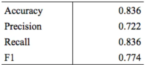
1-1 Number of PALB2 and cancer papers by year [5] . . . 13

4-1 Learning curve for best penetrance/incidence classifier . . . 35

6-1 Learning curves for training and testing for the cohort vs. Integer extractor . . . 45

6-2 Learning curves for training and testing for the carrier vs. noncarrier extractor . . . 47

List of Tables

4.1 Statistics of the penetrance/incidence dataset . . . 31

4.2 Comparing accuracies (percentage correct) of the majority baseline and human performance with the highest recall classifier . . . 32

4.3 Results from the SVM classifier with varying N-grams using optimized parameters for the best version of the classifier . . . 33

4.4 Results from gradually adding domain knowledge to the SVM classifier 34 4.5 Compare removing sequences with and without tagging proteins/DNA 34 4.6 Accuracy for sentence level classification of rationales . . . 36

4.7 Results for classifying abstracts based on rationales . . . 37

6.1 Majority baseline for cohort vs integer . . . 43

6.2 Majority baseline for carrier vs noncarrier . . . 44

6.3 Statistics of the cohort vs. integer dataset . . . 44

6.4 Results from the Cohort vs. Integer SVM classifier with context of 10 words . . . 44

6.5 RCNN vs. SVM for cohort extraction . . . 45

6.6 Statistics of the carrier vs. noncarrier dataset . . . 45

Chapter 1

Introduction

Natural language processing in the context of biology holds much promise, because of the burgeoning amounts of structured and unstructured data [1]. In some cases,

it’s actually necessary to use NLP to automatically process data, when the amount of data is infeasible for humans to manually process. I chose to focus on the problem of

determining relevant cancer-gene association articles. This is a worthwhile problem to investigate, because the number of papers being published in the field is

increas-ing year after year (Figure 1-1), and therefore increasincreas-ing the number of irrelevant abstracts that would be read by human annotators. A classifier that can

automati-cally determine relevant papers can be directly applied to the recently developed All Syndromes Known to Man Evaluator.

1.1

All Syndromes Known to Man Evaluator (ASK2ME)

The All Syndromes Known to Man Evaluator (ASK2ME) is a calculator on a website jointly developed by the Dana Farber Cancer Institute (DFCI) and the Massachusetts

General Hospital (MGH). Given basic patient information such as age, gender, ge-netic mutations, and cancer/surgery history, ASK2ME can estimate the likelihood of

developing various cancers over time. The output is given as a risk curve of develop-ing the cancers for mutation carriers and noncarriers. ASK2ME currently supports

data for 31 genes/variants and 16 cancers.

The ASK2ME website also provides the medical journal articles that the estimates were calculated from. Papers are rated 1 to 5 stars based on the quality of the study.

Quality is primarily based on the number of people that the study tested, i.e. the cohort size. ASK2ME particularly focuses on the number of mutation carriers that

were tested. For example, a paper is rated 4 stars if the number of carriers is at least 200.

1.2

Problem

ASK2ME requires a lot of data from medical journals to generate accurate risk curves.

Previously, human annotators provided data by manually searching for papers on PubMed (and other sources), saving the full text articles, reading them to check

for accuracy, and recording any relevant data from these papers about penetrance, incidence, and other risk factors.

Manually saving and reading articles take a lot of valuable time. Not only that, only 20% of the papers contain relevant data for calculating risk curves, and so a lot

of valuable annotation time is wasted on reading the abstracts of irrelevant papers. Irrelevant papers are also very difficult to remove by merely refining the search criteria

1.3

Goals

The goals of this project were to automate the literature review process for the All Syndromes Known to Man Evaluator. Concretely, I sought to:

1. Automate the abstract gathering process for annotation and future data

gath-ering

2. Develop a text classifier that can determine which abstracts are relevent

3. Extract cohort sizes to be used for rating papers based on quality of the study

1.4

Challenges

The main challenge of this problem was the difficulty of the classification task, even

for human annotators with a strong background in biology, because the definition of "relevance" is very complex, and there is some ambiguity with working with

ab-stracts, because it’s sometimes difficult to judge if a full text article is relevant simply by reading the abstract. Fifteen percent of the abstracts were ambiguous, further

confirming the difficulty of this task.

The difficulty of annotation meant that annotating took a very long time (in-cluding correcting previous annotations). Therefore, I only had around 2500 training

examples to work with. This challenge was partially resolved by having annotators mark rationales, or the sections of the abstract that would support their choice of

relevancy. Marking rationales only doubled the annotation time. In other words, it is much more manageable to mark 1000 abstracts with rationales than 10000 abstracts

without rationales.

The rest of this paper describes the ways that these challenges were overcome to meet the project goals. Chapter 2 summarizes some other methods that would be

applicable to this problem, and how some of these methods were adapted into the project. Chapter 3 describes the methods for building the classifier, including how the

The information extraction methods and results are described in chapters 5 and 6. Finally, chapter 7 provides a conclusion, where I discuss the results, implications and

Chapter 2

Related Work

In this chapter, I further discuss some of the methods I used, which were adapted

from other papers. I primarily focus on methods that use rationales, which was first pioneered in [4]

2.1

Text Classification Methods

I used the SVM model to classify abstracts because of the relatively few training

examples. However, many more avenues (particularly neural models) are open if I were to obtain more data. The methods vary from simply using a stronger model to

classify the processed abstracts to using the sentence-level annotations on rationales.

2.1.1

RCNN for Text Classification

There are many ways to represent the document using neural models. For example, one could feed the words in each document to an LSTM or bidirectional LSTM

network. For classifying penetrance and incidence, I used a recurrent convolutional neural network (RCNN) [2]. This model works particularly well for text classification,

because it incorporates the non-linear interactions between words and phrases by using non-consecutive n-grams as well as the traditional consecutive n-grams. This

mutations" are actually recognized to be similar.

2.1.2

Rationale-Augmented CNN

Given annotations on which sentences are rationales, we can create a straightforward

model that utilizes the sentence-level annotations. Such a method was implemented by Zhang et al [6]. This classifier first converts each individual sentence to sentence

vectors and performs supervised sentence-level classification to determine which sen-tences are rationales. There were three types of sensen-tences: positive rationales,

neg-ative rationales, and neutral sentences. During testing, the model calculates the document vector by taking the weighted average of sentences, where each sentence

is weighted by the probability that the sentence is a rationale. Since there are two probabilities (probability that it’s a positive or negative rationale), the authors

sim-ply took the max of 𝑝(𝑦_𝑠𝑒𝑛𝑖𝑗 = 𝑝𝑜𝑠) and 𝑝(𝑦𝑖𝑗_𝑠𝑒𝑛 = 𝑛𝑒𝑔), where 𝑦𝑖𝑗 is the label for the 𝑗th sentence in the 𝑖th document.

I adapted their work to the SVM context, because fewer examples are required

for SVM. I classified positive rationales and neutral sentences, and if there was a rationale in the document, I classified the document as positive.

2.1.3

Rationalizing Neural Predictions

Relying too much on rationale annotations could hurt success on the main task of document classification. Lei’s rationale neural model [3] can predict the important

parts of each document with absolutely no supervision rationales.

The model uses a cost function that allows the model to jointly learn where the rationale is, while doing the main task. The first component of the cost function is

similar to any other loss function for minimizing error on predictions.

𝐿(𝑧, 𝑥, 𝑦) = ||𝑒𝑛𝑐(𝑧, 𝑥) − 𝑦||2₂

Here, 𝑧 is a vector that indicates which words are part of the ratioanle. There is

consecutive words, so that phrases are chosen, rather than disjoint sets of words.

Ω(𝑧) = 𝜆1||𝑧|| + 𝜆2

∑︁

𝑡

|𝑧𝑡− 𝑧𝑡−1|

The cost function would simply be:

𝑐𝑜𝑠𝑡(𝑧, 𝑥, 𝑦) = 𝐿(𝑧, 𝑥, 𝑦) + Ω(𝑧)

This model is most effective if there are a lot of document annotations to train

on. In the paper, this model was tested on a dataset of 1,580,000 documents. It’s very difficult to obtain that many medical abstracts that are specifically in the field

of cancer, germline mutations, and risk. It would also be immensely challenging to annotate this many medical abstracts because the task is hard, even for medical

doctors.

One could make the following changes to the model to need fewer examples. For

example, changing the word level classifier to sentence level would reduce the number of choices needed to determine which parts are the rationales. Also the loss terms

could be modified so that they incorporate rationale annotations (cross entropy loss) and perhaps need fewer document annotations.

The new cost function may look like this, where 𝑥 now represents a vector of sentence representations, and 𝑧 indicates which sentences are rationales.

𝐿(𝑧, 𝑥, 𝑦) = ||𝑒𝑛𝑐(𝑧, 𝑥) − 𝑦||2₂ Ω(𝑧) = 𝜆1||𝑧|| + ∑︁ 𝑖∈𝑠𝑒𝑛𝑡𝑒𝑛𝑐𝑒 [log 𝑝(𝑧𝑖 = 1|ˆ𝑧𝑖 = 0) + log 𝑝(𝑧𝑖 = 0|ˆ𝑧𝑖 = 1)] 𝑐𝑜𝑠𝑡(𝑧, 𝑥, 𝑦) = 𝐿(𝑧, 𝑥, 𝑦) + Ω(𝑧)

Chapter 3

Classifying Penetrance and Incidence

Methodology

The ASK2ME calculator requires data from medical journal articles that provide statistics for associations between germline genetic mutations and cancers. Previously,

this data was obtained by human annotators manually searching and saving full text articles, and filling in spreadsheets with the necessary data after reading the full text

article. This takes a tremendous amount of time, because more than half of the papers obtained by searching on PubMed (even with a highly refined query), are not

relevant. I developed a classifier for automatically finding relevant papers.

3.1

Definition of Relevance

In this context, a paper is relevant if it discusses the risk of germline mutation carriers developing a cancer or syndrome. Germline mutations are those caused by genetics,

rather than somatic mutations caused by external factors. Specifically, we defined a paper as relevant if it contains data for penetrance and/or incidence.

A paper is relevant to penetrance if it describes the risk of cancer among germline

mutation carriers. Incidence papers, in contrast, describe the percentage of muta-tion carriers in a populamuta-tion. Relevant papers must contain specific risk objects, i.e.

hazard ratio (HR), odds ratio (OR), relative risk (RR), cumulative risk (CR), and standardized incidence ratio (SIR). If there is any data that would allow one to

cal-culate these percentages or risk objects, the paper is also relevant, e.g. if a paper mentions the number of people who had the mutation and the disease.

To avoid including redundant studies, relevant papers must also be an original

paper, rather than a literature review of other articles. However, comprehensive reviews that additionally used their own techniques to calculate risk objects should

be marked as relevant. Note that there is a fine line between reviews that should or should not be included, which could potentially lead to ambiguity.

Additionally, a paper is relevant if it provides associations between mutations and cancers, rather than polymorphisms and cancers. (If it provides data on both, it is

still a relevant paper.) A polymorphism is a DNA sequence change that is present in more than 1% of the general population.

Overall, the definition of relevance is very complex, and identifying relevant papers a difficult task for humans, even those with expertise in the domain.

3.2

Entrez Direct

Previously, human annotators saved full text articles (typically PDFs) manually. It’s

difficult to automatically obtain these PDFs, because it may involve scraping web pages. Even after obtaining PDFs, converting PDFs to machine-readable text files

is often very noisy due to varying formats, figures, and tables. In contrast, abstract texts are much more feasible to obtain.

Entrez Direct (EDirect) is a Unix command line package that allows one to search through the PubMed database. EDirect can accept a query and output the results in

XML format, and also supports commands to extract some common fields (example below). The majority of entries for papers on the Pubmed database contains a field for

the full abstract text, so I decided to use this package to automatically pull abstracts for annotators to annotate.

-e l -e m -e n t A b s t r a c t / A b s t r a c t T -e x t | i c o n v - c - f utf -8 - t a s c i i ) "

3.3

Automated Data Collection

I built a tool on top of EDirect that can accept a query, search through the database, and automatically populate a CSV with various fields, e.g. journal title, paper title,

author, abstract text, query, timestamp, etc.

To generate a table using this tool, first initialize the table with all the column names, which one can supply under "scripts/columns.txt". This will create a new file

named "database/gene-cancer.csv".

1 s c r i p t s / i n i t _ t a b l e . sh g e n e c a n c e r

You can then fill the table with results from a particular query with the following command.

1 s c r i p t s / f i l l _ t a b l e . sh ’ query ’ g e ne c a n c e r

In order to avoid duplicates within the same table, the list of pubmed id’s are

saved under the cache folder for the particular gene and cancer pair.

3.4

Data Annotation

Annotations were done from scratch by collaborators at DFCI and MGH. Each of the six annotators read the abstracts of papers to determine whether the paper would be

relevant or not. For each abstract, annotators marked penetrance or incidence. If a paper was marked as a 1 for either of these categories, it is relevant. Annotators also

marked whether the abstract has data on risk of a second cancer developing in the same organ or different organ, whether the paper exclusively discusses polymorphisms

(in which case, it wouldn’t be relevant), and whether the paper is a meta-analysis.

Initially, the annotations were done with respect to cancer and gene, meaning that an abstract was only marked as relevant if it contained an association with the given

positives, because queries about a specific cancer and gene combination often pulls up abstracts about other cancers / genes, e.g. if the cancer / gene were mentioned

in the abstract in the background. To increase the number of positive examples to be used for training, the annotations were done with respect to just penetrance or

incidence for cancer and gene, regardless of which cancer or gene it was. All previous annotations were redone to fit this new rule.

The classification task is immensely difficult for humans. This leads to a lot of time needed for annotating, and gives room for a lot of mistakes, despite giving the

annotators a highly specific definition of what "relevance" means. Because of this, we added a column for marking ambiguous abstracts, where ambiguous means that 2

or more annotators disagreed on a row, or 1 annotator thought there wasn’t enough information in the abstract to determine whether a paper is relevant. Fifteen percent

of the abstracts were ambiguous, further confirming the difficulty of this task.

3.5

SVM Classifiers

There were several iterations of this classifier. The main features are based on bag of words features. In later versions of the classifier, domain knowledge was added

in order to reduce the vocabulary size and help the classifier understand unknown words.

3.5.1

Implementation

The algorithm was implemented in Python 2.7 using packages from sklearn. The basic classifier is a SGDClassifier with hinge loss, L2 penalty, and 6 iterations. For

featuriz-ing based on bag of words, I tested both the CountVectorizer and TfidfVectorizer that incorporates stop words. TfidfVectorizer gave 6% higher F1/recall, and so this was

used throughout experimentation. For each trial, I use sklearn’s GridSearchCV pack-age to automatically find the optimal parameters for the SGDClassifier as the model

3.5.2

N-gram Bag of Words

Initially, I only used bag of words on unigrams, resulting in a very basic model. I saw substantial improvement after extending the model to higher n-grams. I used the

TfidfVectorizer with sublinear tf. I specified stopwords to be nltk’s English stop words set. As I was developing the model, I used (1, 3)-grams (unigram, bigram, trigram).

After finishing the text processing steps (below), I tested five different n-gram ranges: (1), (1, 2), (1, 3), (1, 4), and (1, 5).

3.5.3

Basic Text Processing

A significant part of optimizing the classifier was determining how to best process

the text. In the first iteration of the classifier, I simply converted the abstracts to lowercase to preprocess. I also inserted spaces between parentheses, commas, periods,

and other punctuation marks. Some abstracts also contained special characters that unicode doesn’t recognize. These were also removed.

3.5.4

Convert Numbers

Statistics related to penetrance and incidence are often presented in similar ways. For

example, risk objects, such as relative risk are presented as "relative risk (number)". Bag of words would recognize "relative risk (1.6)" as a different trigram than "relative

risk (2.5)", even if both are similar signals for penetrance. To account for this, I generalized the numbers by replacing them with tags: "percent", "decimal", "ratio",

"num". Additionally, I converted numbers in the form of words, e.g. "twenty-seven", to the "num" tag.

To convert text numbers, I hard coded a list of number words, and if a word is part of the list, I converted it to the "num" tag. In order to convert multi-word

numbers (such as "thousand two hundred and one"), I replaced consecutive "num" tags to just "num", and replaced "num and num" to "num".

Tag Regex

percent [0-9]*[.]?[0-9]*%

decimal [0-9]*˙[0-9]+

ratio [0-9]+[ ]?[:/][ ]?[0-9]+

num [0-9]+[.]?

3.5.5

Generalize Genes, Cancers, Syndromes, and Organs

Recall that abstracts are marked as relevant if it discusses penetrance or incidence

for any gene / cancer combination. Hence, it’s in our best interest to generalize gene and disease names. With the help of collaborators from MGH and Dana Farber,

we generated a list of genes related to cancers, syndromes, and cancers, and their synonyms. The initial list of cancers and genes were based on the list on the ASK2ME

calculator. More were added as abstracts were being reviewed.

Using the hard coded list of genes and cancers, each entity name was replaced in the abstract text. The list of entities were first ordered by length of each phrase,

in order to avoid substrings of words being replaced before the phrase was replaced. There are many instances of "gene_name gene" (e.g. "MLH1 gene"). Therefore,

"gene gene" was replaced by "gene". Similarly for "syndrome syndrome", etc.

Some abbreviated gene names appear as substrings in other words. In some cases, this is fine. For example, "ATM-positive" should still be converted to "gene-positive".

However, when "atm" appears as part of the word "treatment", we should not convert it to "gene". To avoid these cases, I simply split the list of genes into two, one with

capitalized abbreviations, and the other that are either words or phrases. I use the gene abbreviations list before converting the text to lowercase. After converting to

lowercase, I then use the other lists to convert other entities.

There were also many instances of two different cancers named simultaneously, e.g. "breast and ovarian cancer" or "breast/ovarian cancer". These would become

"breast and cancer" after generalizing the cancer names. In order to also generalize the first cancer, we created a list of organs and used it to convert organ names as well.

3.5.6

Generalize Variant Names

Variants are different versions of genes caused by insertions, deletions, and duplica-tions. For example, a variant of the CHEK2 gene is 1100delC.

It is difficult to generate a concrete list of all possible variants, because there are so many possibilities. However, variants are often written in well-defined patterns. The

collaborators at MGH provided a list of 1918 example variants and variant patterns. I used this list to come up with regex expressions that should be able to detect most

variants. The accuracy for the regex searching wasn’t formally evaluated, but the medical collaborators confirmed that the variants I find through regex indeed are

variants.

If a word looked like a variant based on the regex pattern, or was part of the

list of 1918 variants, I replaced the string with the word "variant". The list of regex expressions are below:

1 c \. 2 C \. 3 C -[0 -9]+ 4 c -[0 -9]+ 5 [0 -9]+[ a c t g A C G T ]+ $ 6 [0 -9]+ _ [0 -9]+ del 7 5 ’ UTR 8 5 UTR 9 [0 -9]+ del 10 [0 -9]+ ins 11 IVS 12 del [0 -9]+ 13 del e x o n 14 del e n t i r e 15 Del E x o n 16 Del e x o n 17 del p r o m o t e r 18 del p r o m o t o r 19 dup p r o m o t e r 20 dup p r o m o t o r 21 ex [0 -9]+ del 22 ex [0 -9]+ ins 23 ex [0 -9]+ dup 24 [ Dd ] e l e t i o n 25 [ Dd ] u p l i c a t i o n 26 [ Ii ] n s e r t i o n 27 dup e x o n 28 dup p r o m o t e r e x o n 29 Ex [0 -9]+ 30 EX [0 -9]+ 31 [ A D G H I K L M N P Q R S T V Y q ][0 -9]+ 32 E [0 -9]+ 33 [ -+]?[0 -9]+[+ - _ ] [ -+ ] ? [ 0 - 9 ] + dup 34 [ -+]?[0 -9]+[+ - _ ] [ -+ ] ? [ 0 - 9 ] + ins 35 [ -+]?[0 -9]+[+ - _ ] [ -+ ] ? [ 0 - 9 ] + del 36 [+ -]?[0 -9]+[+ - _ ] [ 0 - 9 ] + \ _ [0 -9]+] 37 3 ’ t e r m i n a l 38 .*[0 -9] ins 39 .*[0 -9] del 40 .*[0 -9] dup

3.5.7

Generalize Protein Changes and Chromosomes

From looking at some false positives and negatives, it became apparent that the classifier made the mistakes because it didn’t recognize some strange strings as protein

changes (amino acid changes), or chromosomes.

I requested some examples of protein changes from our medical collaborators.

Us-ing the set of examples, and rules that they come up with, I was able to develop another set of regexes for detecting protein changes. Protein changes typically (but

not always) starts with the prefix "p.". They also usually contain an amino acid ab-breviation, an integer, and then another amino acid abbreviation. The list of regexes

is below.

1 [ Pp ]\.

2 [ Ala | Arg | Asn | Asp | Cys | Glu | Gln | Gly | His | Ile | Leu | Lys | Met | Phe | Pro | Ser | Thr

| Trp | Tyr | Val ] [ 0 - 9 ] + [ Ala | Arg | Asn | Asp | Cys | Glu | Gln | Gly | His | Ile | Leu | Lys | Met | Phe | Pro | Ser | Thr | Trp | Tyr | Val ]

3 [ Ala | Arg | Asn | Asp | Cys | Glu | Gln | Gly | His | Ile | Leu | Lys | Met | Phe | Pro | Ser | Thr | Trp | Tyr | Val ][0 -9]+ del

I used this list to convert protein changes in the abstract text to a "protein" tag.

Similarly, abstracts often contain strings representing chromosomes. To detect these, I used another regex:

1 \ v e r b ! ( [ 1 - 9 ] [ 0 - 9 ] ? [ pq ] [ 0 - 9 ] [ 0 - 9 ] ? ( \ . [ 1 - 9 ] [ 0 - 9 ] ? ) ?) !

3.6

Rationales

A rationale is a subset of sentences from the abstract that is concise and often provides a strong enough signal to classifiy. This is similar to Lei et al’s definition of rationales

3.6.1

Annotation

The annotators marked all sentences that were relevant to penetrance or incidence to justify positive decisions. In this classification task, it’s difficult to find "negative"

rationales, because an abstract is usually classified as irrelevant because of lack of a positive signal, rather than because it contains something that makes it negative.

Hence, no rationales were provided for negative examples.

The annotators had varying styles for marking rationales. Some marked sentences

as relevant because the background or method appeared to suggest that it will contain penetrance or incidence results. Others marked a sentence only if it explicitly

men-tioned numbers about penetrance or incidence. Despite the varying styles, utilizing rationales may give the classifier valuable insight as to what relevant abstracts look

like.

3.6.2

Hierarchical Model

I adapted the rationale-augmented neural text classifier that was developed by Ye

Zhang, et al (explained more in the Related Works chapter). The original paper showed the use of positive, negative, and neutral rationales, so for each sentence,

they took the max of 𝑝(𝑦_𝑠𝑒𝑛𝑖𝑗 = 𝑝𝑜𝑠) and 𝑝(𝑦_𝑠𝑒𝑛𝑖𝑗 = 𝑛𝑒𝑔). For this problem, there are only positive and neutral rationales.

I implemented a simple SVM version of this model that works for positive and neutral rationales. I randomly shuffled the data, and used the sentences from 2000

ab-stracts for training, and the rest of the 500 abab-stracts for testing. I repeated randomly shuffling and splitting the data for 10 trials.

I first train the model by feeding in each sentence at a time, converting each sentence using preprocessing, and using the rationale annotations to classify sentences

as neutral or positive. Using the trained classifier, I predict rationales in the test abstracts. If there is any sentence that is classified as a positive rationale, I predict

Chapter 4

Classifying Penetrance and Incidence

Results

4.1

Dataset Statistics

There were many abstracts that were marked as "ambiguous" or "polymorphism". Ambiguous abstracts are ones that human annotators have disagreements on, or has

a very weak signal for relevance. Polymorphism abstracts should definitely be irrele-vant, but are also often difficult to classify by humans because they often look similar

to penetrance/incidence abstracts.

Also the dataset was biased in that there were significantly more negative examples

than positive ones. The breakdown of the data is shown in Table 4.1. There were some abstracts that had blank abstracts, such as the entries on PubMed that didn’t

have the abstract in the field.

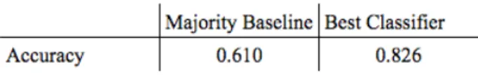
Table 4.2: Comparing accuracies (percentage correct) of the majority baseline and human performance with the highest recall classifier

Halfway through annotating, the annotations were analyzed and corrected by

having more than one annotator look at each row. At the time, 11% of the abstracts either required corrections from disagreements, or was marked as ambiguous by an

annotator. Since then, the annotations have been corrected with a more rigorous definition of relevance, but note that there may still be mistakes in the data.

4.2

Evaluation

The classification was evaluated accuracy (percent correct), precision, recall, and F1

score. The focus was primarily on the recall score, since the goal was to achieve a high recall score with a reasonable F1 score.

For experimentation, all ambiguous/polymorphism abstracts were first discarded from the dataset. Ambiguous abstracts can be classified either way by annotators,

so they are meaningless to evaluate on. There are very few polymorphism abstracts, and so very few training examples for the classifier to learn the tricky definition of

polymorphism, so this was also left for a later task. There were 2532 abstracts that are neither polymorphism nor ambiguous.

4.3

SVM Classifier Results

This section presents and discusses the results from experiments for testing vari-ous n-grams and gradually applying domain knowledge to ease understanding. The

classifier with the highest recall score was the one that substituted all tags during the preprocessing step of the data. The best version of the classifier also beats the

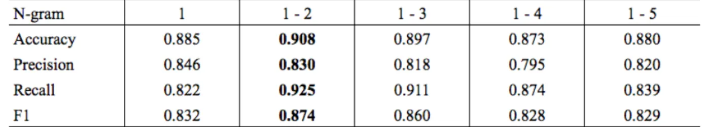
Table 4.3: Results from the SVM classifier with varying N-grams using optimized parameters for the best version of the classifier

4.3.1

N-gram Bag of Words

Various n-gram ranges were evaluated using 5 trials. In each trial, the data array

was randomly shuffled using numpy random seeds, and 2332 abstracts were used to train. The rest of the 200 abstracts were saved for testing. Because the 200 abstracts

were randomly selected using numpy random seeds, the same abstracts were used for testing the various n-gram ranges. These ranges were tested on fully preprocessed

abstracts (i.e. abstracts with number, gene, cancer tags, etc.)

Table 4.3 compares the accuracy, precision, recall and F1 scores across 5 different n-gram ranges. I determined that using a combination of unigrams and bigrams was

the most effective, although using (1, 2, 3)-grams had very similar results. This may be because many longer phrases are condensed to a single word tag. For example

Mutl Homolog 1, which is a longer phrase for the MLH1 gene, is replaced by the word "gene" after preprocessing abstracts. Hence, unigrams and bigrams may have been

sufficient for getting good results, without overfitting on the training set by using longer n-grams.

4.3.2

Domain Knowledge

I next demonstrate that adding domain knowledge to assist the classifier was beneficial to the recall score. The differences between some of the steps were smaller, and hence

often depended on the trials. To obtain a more exact measure, evaluation for this section was done using 10-fold cross validation. Each step was done using the (1,

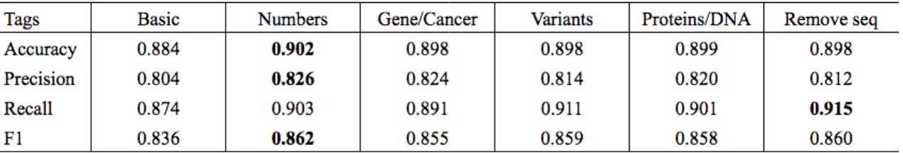
Table 4.4: Results from gradually adding domain knowledge to the SVM classifier

Table 4.5: Compare removing sequences with and without tagging proteins/DNA

each step, the model’s optimal max degrees of freedom and classifier’s 𝛼 were selected using sklearn’s GridSearchCV.

Table 4.4 contains the results. The definitions for each column are below.

Basic Convert text to lowercase, insert spaces between punctuation marks, remove

foreign characters

Numbers Basic processing and add decimal, percent, ratio, and num tags for the corresponding types of numbers.

Gene/Cancer All of above and convert phrases and words representing genes,

can-cers, syndromes, and organs to the corresponding tags.

Variants All of above and tag variants.

Proteins/DNA All of above and tag protein changes and chromosome names.

Remove seq All of above and convert sequences of entities, e.g. "gene, gene, and gene" would become "gene".

It appears that adding protein and chromosome tags decreased the F1 score.

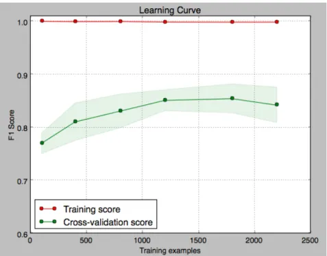
Figure 4-1: Learning curve for best penetrance/incidence classifier

the performance dropped (Table 4.5). Hence, the classifier with the highest recall is

the classifier that tags everything including proteins and DNA, and removes sequences of tags.

Figure 4-1 displays the learning curve for training and testing for the best classi-fier. The curve levels off, indicating that the SVM model is saturated. However, far

more examples would be needed for a neural model, meaning that we could reach a higher F1 score based on the current text processing steps.

4.4

Rationale Model Results

In this section, I discuss both the sentence-level classification performance of

ratio-nales, and the performance of the rationale-incorporated SVM model. The results below are based on 10 trials generated by numpy random seeds, with a test set size

Table 4.6: Accuracy for sentence level classification of rationales

4.4.1

Sentence-Level Results

The model had immense difficulty identifying rationale sentences from supposedly

neutral ones (Table 4.6). This may be because each of the six annotators had very different styles for annotating rationales. Some annotators marked only sentences

that contained statistics related to penetrance or incidence in the results portion of the abstract. Other annotators included background or methods sentences, as long

as the sentences implied that the focus of the study was on risk.

After analyzing the mistakes made by the sentence-level classifier, it appeared

that many of the false negatives actually appeared to be similar to rationales. Hence, the low F1 score for this classifier isn’t a huge issue, as long as one sentence in each

relevant abstract is labeled as a rationale.

4.4.2

Document-level Results

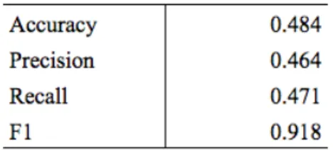
The F1 score was .774, which is lower than even the SVM model with basic text

processing (presented in the previous chapter). This lower result could simply be because the annotations for the rationales were so noisy. Note that the recall score

(.836) much higher compared with the low precision score. Because the goal is to maximize the recall score (with reasonable F1 score), changing the rational

annota-tions so that more sentences are labeled as rationales would improve the score. Being consistent with rationale annotations would improve precision.

Moving away from a method that relies so much on correct rationale annotations

would be ideal however. There are neural techniques which can do this, such as Lei et al’s word-level model that predicts which segments of the document is the rationale.

Table 4.7: Results for classifying abstracts based on rationales

the rationale [3], which would be useful for a small dataset, like in this particular problem. Adding loss terms to incorporate the rationale supervision could also be

Chapter 5

Extracting Cohort Size Methodology

Another goal of this project was to extract the cohort sizes of the study. Ideally, the

developers of ASK2ME wanted very detailed labels on each type of cohort size for each gene/cancer pair: total, total with disease, total healthy, mutation carriers with

disease, noncarriers with disease, carriers that are healthy, and noncarriers that are healthy. However, annotating these detailed cohort sizes take a lot of time. Also,

usually only some of the cohort sizes are provided in the abstract.

I decided to tackle a simpler problem of first determining whether a number in the abstract is a cohort size at all. After a achieving high F1 score for this, I then

moved onto simply separating the number of carriers with the number of noncarriers.

5.1

Annotation

A naive way to annotate the cohort sizes is having annotators read the entire abstract

and record all numbers that are cohort sizes. However, notice that cohort sizes must be nonnegative integers, so annotators only need to read the sentences that have

nonnegative integers (or words representing integers). Furthermore, I noticed that only a few surrounding words are needed to determine whether a number is a cohort

size. From empirical testing, it seemed that a context of 10 words is sufficient. This means that annotating whether a number is a cohort size or not only requires reading

Knowing this, I wrote a Python script that prints out snippets of text from the abstract, each containing an integer with a context of 10 words. I gave the snippets

to two annotators to annotate two columns: is_cohort_size and ambiguous. Anno-tating these snippets was much more efficient. It would take days for the annotators

to read 1500 full abstracts. However, reading all the snippets from these abstracts took only a few hours. Annotating 10 snippets took less than one minute.

Once I got a high F1 score for predicting whether a number is a cohort size or not, I wanted to see how well I could predict whether the cohort size describes the

number of carriers or noncarriers. I wrote another Python script that went over the annotated file and removed all rows that contained snippets not about cohort

sizes. I then extended the context to the entire sentence, because it’s likely that more information may be needed to distinguish carrier sizes and noncarrier sizes. I gave

this to the annotators to annotate is_carrier_size and ambiguous.

5.2

Cohort Size Classification

After realizing that a small context is sufficient to detect cohorts, I simply used

the SVM classifier with (1, 2, 3)-gram bag of words on the short snippets. I used similar text processing as I used for classifying abstracts for penetrance and incidence.

During preliminary testing, the CountVectorizer appeared to perform slightly better the TfidfVectorizer. Hence, the CountVectorizer was used for the experiments. Each

snippet has the candidate cohort size surrounded by 10 words on either side (4 to 5 words per side).

Clasifying the snippets this way is a very simple method that can still capture

both the forward and backward contexts. I also tested Lei’s RCNN model, which is performs especially well at text classification. However, this didn’t perform as high

as the SVM model, probably because of few test examples.

An alternative direction is to use a bidirectional LSTM which also captures the backward and forward contexts. However, when the RCNN model performed worse

for this task.

5.3

Carrier vs. Noncarrier Classification

I used the same method as the above to distinguish carrier cohort sizes from noncarrier

cohort sizes. Rather than using the entire sentence as the context, I wrote a script that picked out the current candidate word, and tested various context lengths surrounding

the candidate to find the optimal context length. I tested context lengths of 4 through 8.

Chapter 6

Extracting Cohort Size Results

There were two datasets, one comprising snippets of 10 words surrounding each integer in the abstract text with labels on whether it is a cohort size or not, the other

comprising sentences that contain cohort sizes, with annotations as to whether the highlighted word describes the number of carriers or noncarriers. The breakdown of

each dataset is given in the tables below. Evaluation was again done on F1, recall, precision, and accuracy. I ran 10 trials and averaged the metrics. In each trial, I used

a test set size of 200 snippets.

Both classifiers perform much higher than the majority baseline, particularly the cohorts extractor.

6.1

Cohort Size vs. Integer Extraction

This section presents the dataset statistics and performance of the classifier that dis-tinguishes cohort size numbers from other positive integers. The dataset was quite

large with over 3000 snippets of 10 words surrounding each candidate cohort size. Per-haps because of the large dataset, and because this task is also very easy for humans,

Table 6.2: Majority baseline for carrier vs noncarrier

Table 6.3: Statistics of the cohort vs. integer dataset

the metrics were quite high (Table 6.4). The learning curve (Figure 6-1) indicates

that there were enough data points to saturate the learning. The learning curve was calculated using sklearn’s learning curve package using a 5-fold cross validation.

I also compared the performances of RCNN and SVM. RCNN performed worse

than SVM for all metrics (Table 6.5), probably because of the relatively few training examples.

6.2

Carrier vs. Noncarrier Extraction

This is a much more difficult task that above. The vocabulary used to describe cohort sizes and other integers is very different, which is why the machine is so

good at detecting the difference through bag of words. However, the vocabulary that describes mutation carrier cohort sizes is very similar to that which describes

noncarrier sizes. There were also much fewer examples for the carrier vs. noncarrier extraction, because the dataset was derived from further annotation on a subset of

Table 6.4: Results from the Cohort vs. Integer SVM classifier with context of 10 words

Figure 6-1: Learning curves for training and testing for the cohort vs. Integer extrac-tor

Table 6.5: RCNN vs. SVM for cohort extraction

Table 6.7: Results from the Carriers extractor with varying contexts

the cohort vs. integer dataset.

For this task, various context lengths were tested. For example, a context length of 7 indicates 3 words on either side of the candidate word. The results are reported

in Table 6.7. The best context was a context of 6 words, closely followed by a context of 7.

I wanted to check if the relatively low F1 score was because more training ex-amples were needed. However, the learning curve was saturated. This is probably

because this is generally a more difficult task than merely determining which numbers represent cohorts, because you have to further distinguish between cohorts. Also, the

model was a very simple one, so there is promise in investigating other methods. For example, one could use bidirectional LSTMs to similarly capture the context from

either side of the candidate cohort, though this method would require more training examples.

Figure 6-2: Learning curves for training and testing for the carrier vs. noncarrier extractor

Chapter 7

Conclusion

The contributions of the project can be directly applied to fully automating the literature review process for the All Syndromes Known to Man Evaluator (ASK2ME).

This can significantly reduce the time it takes to gather enough data to calculate risk curves for cancers based on germline mutations. The contributions discussed in this

thesis were:

1. Design and build a system for creating annotation tables and preannotating abstracts to expedite annotations

2. Build a penetrance/incidence classifier that achieves high performance on de-sired metrics (F1 = 0.86, recall = 0.905) using domain knowledge

3. Implement a baseline approach that utilizes rationales for the text classification teask

4. Develop strong extractors for cohort size (F1 = 0.89) and carrier cohorts (F1 = .753).

The accuracy of the penetrance/incidence classifier was 89.8%, outperforming the

human performnace of 85%. Despite the high performance, there is much promise for further improvement by incorporating rationales, which can help the model focus on

version of Lei’s rationale model (described in Chapter 2), especially after procuring more annotations.

The thesis also explored some simple models for determining cohort sizes and carrier cohorts. However, the structure for presenting this type of data is perhaps more

limited than the highly various structures or styles of writing that entire abstracts come in. Hence, there could be ways to bootstrap these limited sets of patterns using

some dependency structures. Also, distinguishing carrier cohorts from noncarrier cohorts was found to be a much more difficult task. This could be further improved by

having a better representation of the context words, such as feeding the words through a bi-directional LSTM. Overall though, this paper presents very strong baselines for

Bibliography

[1] George Karystianis, Kristina Thayer, Mary Wolfe, and Guy Tsafnat. Evaluation of a rule-based method for epidemiological document classification towards the automation of systematic reviews. Journal of Biomedical Informatics, 70, 2017.

[2] Tao Lei, Regina Barzilay, and Tommi Jaakkola. Molding cnns for text: non-linear, non-consecutive convolutions. In Empirical Methods in Natural Language Processing (EMNLP), 2015.

[3] Tao Lei, Regina Barzilay, and Tommi S. Jaakkola. Rationalizing neural predic-tions. CoRR, abs/1606.04155, 2016.

[4] Jason Eisner Omar F. Zaidan and Christine Piatko. Using âĂIJannotator ratio-nalesâĂİ to improve machine learning for text categorization. NAACL, 2007.

[5] Jennifer K. Plichta, Molly Griffin, Joseph Thakuria, and Kevin S. Hughes. WhatâĂŹs new in genetic testing for cancer susceptibility? Oncology, 2016.

[6] Ye Zhang, Iain James Marshall, and Byron C. Wallace. Rationale-augmented convolutional neural networks for text classification. CoRR, abs/1605.04469, 2016.