HAL Id: hal-00296090
https://hal.archives-ouvertes.fr/hal-00296090
Submitted on 6 Dec 2006
HAL is a multi-disciplinary open access
archive for the deposit and dissemination of
sci-entific research documents, whether they are
pub-lished or not. The documents may come from
teaching and research institutions in France or
abroad, or from public or private research centers.
L’archive ouverte pluridisciplinaire HAL, est
destinée au dépôt et à la diffusion de documents
scientifiques de niveau recherche, publiés ou non,
émanant des établissements d’enseignement et de
recherche français ou étrangers, des laboratoires
publics ou privés.
GCM
H. Tost, P. Jöckel, J. Lelieveld
To cite this version:
H. Tost, P. Jöckel, J. Lelieveld. Influence of different convection parameterisations in a GCM.
At-mospheric Chemistry and Physics, European Geosciences Union, 2006, 6 (12), pp.5475-5493.
�hal-00296090�
www.atmos-chem-phys.net/6/5475/2006/ © Author(s) 2006. This work is licensed under a Creative Commons License.
Chemistry
and Physics
Influence of different convection parameterisations in a GCM
H. Tost, P. J¨ockel, and J. Lelieveld
Atmospheric Chemistry Department, Max-Planck Institute of Chemistry, P.O. Box 3060, 55020 Mainz, Germany Received: 17 August 2006 – Published in Atmos. Chem. Phys. Discuss.: 26 September 2006
Revised: 30 November 2006 – Accepted: 1 December 2006 – Published: 6 December 2006
Abstract. In global models of the atmosphere convec-tion is parameterised, since the typical scale of this pro-cess is smaller than the model resolution. Here we address some of the uncertainties arising from the selection of dif-ferent algorithms to simulate this process. Four difdif-ferent parameterisations for atmospheric convection, all used in state-of-the-art models, are implemented in the model sys-tem ECHAM5/MESSy for a consistent inter-comparison and evaluation against observations. Relatively large differences are found in the simulated precipitation patterns, whereas simulated water vapour columns distributions are quite simi-lar and close to observations. The effects on the hydrological cycle and on the simulated meteorological conditions are dis-cussed.
1 Introduction
The adequate treatment of convection in computer models of the Earth’s atmosphere is one of the major uncertainties in weather and climate simulations (Randall et al., 2003). Convection is crucial for the stabilisation of the atmosphere, and for the vertical redistribution of energy, water vapour and chemical species throughout the troposphere. It characterises large circulation systems (e.g., Hadley and Walker circula-tion) and indirectly influences the dynamics of the strato-sphere through the triggering of gravity waves. Within the Inner Tropical Convergence Zone (ITCZ) convection largely determines the daily weather. Only in high resolution models with grid sizes of about 1 km×1 km it is possible to resolve individual clouds, while in all other models, especially in contemporary general circulation models (GCMs), convec-tion must be described with the help of parameterisaconvec-tions. Considerable efforts in parameterising convection have been
Correspondence to: H. Tost
undertaken in the last decades (Arakawa, 2004, and refer-ences therein). Consequently, a large variety of convection schemes is available and applied in GCMs. They are often based on different assumptions, (e.g. Arakawa and Schubert, 1974; Kuo, 1974; Tiedtke, 1989; Hack, 1994; Zhang and McFarlane, 1995; Emanuel and Zivkovic-Rothman, 1999; Donner et al., 2001; Bechtold et al., 2001; Lin and Neelin, 2002; Nober and Graf, 2005), each of them having strengths and weaknesses (Arakawa, 2004). The so-called “super-parameterisation” approach (Grabowski and Smolarkiewicz, 1999; Grabowski, 2004) might overcome some of the weak-nesses (Randall et al., 2003), but since significantly more computational effort is required, hence application in atmo-spheric chemistry general circulation models (AC-GCM) is not feasible. It is important to analyse the influence of con-vection schemes on the simulated climate system. Inter-comparisons of convection schemes in the past have mostly been accomplished with single column models (e.g. Ghan et al., 2000; Xie et al., 2002) and focused on specific con-ditions. According to Randall et al. (1996) this has the ad-vantage of limited amounts of data (for both models and ob-servations) to be compared and an easier identification and separation of individual effects. However, single column studies provide only limited information on the impact of a convection scheme in a GCM, in which basically all at-mospheric conditions occur. Anyhow, convection parameter-isations mainly address the influence of the convective ac-tivity on the larger circulation, while associated processes like mass-balancing subsidence are described in less detail in most of the present parameterisations. In reality convective events can be organised into larger systems (mesoscale con-vective systems) (Houze, jr., 2004). This self-organisation cannot be simulated with most of the present convection parameterisations, even though some approaches to include such effects have already been undertaken (e.g. Donner et al., 2001; Nober and Graf, 2005). Only few previous compar-isons of convection schemes focusing on the global scale
im-pact have been accomplished. A study by Lee et al. (2003) for idealised (aqua-planet) and realistic conditions concluded large differences between the individual parameterisations. Mahowald et al. (1997) investigated the influence of different convection schemes on tracer transport in a chemistry trans-port model (CTM), although they used different input data for their simulations. Therefore the discrepancies between the different results cannot solely be attributed to the influ-ence of the convection parameterisation. Furthermore the in-fluences of the selected scheme on the dynamics and climate cannot be addressed in a transport model driven by offline-computed meteorological data. In this study four different convection parameterisations are implemented in a GCM, accounting for feedbacks on the simulated meteorology. In Sect. 2 the model and the convection schemes are briefly de-scribed; an overview about the simulation setup is given in Sect. 3. The results in Sect. 4 are subdivided into two parts: in 4.1 we present the influences on the hydrological cycle, and in 4.2 we analyse the impacts on the simulated mete-orology. Our conclusions are given in Sect. 5. The main focus of this study is an analysis of the influences of the con-vection schemes on the simulated meteorological conditions of present-day climate and the hydrological cycle. An ac-curate description of the water distribution is important for many processes in the atmosphere including the chemistry. An accurate chemical weather forecast is only possible if the hydrological cycle is well represented by the model. In com-parison with climate modelling with a focus on statistical re-sults, in atmospheric chemistry modelling it is particularly important to accurately simulate the seasonal precipitation and the inter-annual variability.
2 Model description
2.1 Atmospheric chemistry GCM
The AC-GCM ECHAM5/MESSy system combines the GCM ECHAM5 (Roeckner et al., 2006; Hagemann et al., 2006; Wild and Roeckner, 2006) (version 5.3.01) and MESSy (version 1.1), the Modular Earth Submodel System (J¨ockel et al., 2005). ECHAM5 calculates the atmospheric flow in spectral representation with the prognostic variables vorticity, divergence, temperature, the logarithm of the sur-face pressure, specific humidity, cloud water, and cloud ice. The processes of radiation and cloud microphysics are pa-rameterised. In the vertical a hybrid pressure coordinate sys-tem is applied. Advection is calculated with the Lin and Rood (1996) algorithm. The processes of large-scale con-densation (cloud and precipitation formation) are calculated based on work of Lohmann and Roeckner (1996) and Tomp-kins (2002). The detailed description of the physical pro-cesses can be found in the ECHAM5 documentation (Roeck-ner et al., 2003, 2004). MESSy is described by J¨ockel et al. (2005), and the first application of ECHAM5/MESSy as
AC-GCM including a more detailed model description is pre-sented in J¨ockel et al. (2006). At present MESSy contains submodels for atmospheric chemistry, transport, their feed-back on the meteorology, and diagnostic tools.
2.2 Convection parameterisations
ECHAM5 includes the convection parameterisation of Tiedtke (1989) in three different configurations:
– The Tiedtke (1989) scheme with modifications by Nor-deng (1994) (further denoted as T1). This scheme is used as the default convection parameterisation. – The original Tiedtke (1989) scheme without any
modi-fications (denoted as T2).
– The original Tiedtke (1989) scheme with a so-called hy-brid closure (further denoted as T3).
For this study, these schemes have been extracted from ECHAM5, recoded according to the MESSy standard and equipped with a flexible interface, and three additional con-vection schemes have been included via the same interface:
– the convection parameterisation of the operational ECMWF model (IFS cycle 29r1b, further denoted as EC) (Bechtold et al., 2004, and references therein), which is a further development of the Tiedtke (1989) scheme;
– the Zhang-McFarlane-Hack scheme (Zhang and McFar-lane, 1995; Hack, 1994) (ZH) as applied in the MATCH model (Rasch et al., 1997; Lawrence et al., 1999); – the scheme of Bechtold et al. (2001), further denoted as
B.
All convection parameterisations have been implemented in the modularised approach of MESSy. The interface col-lects the required input data from the base model (GCM) and returns the results of the convection calculations back to the GCM.
Although (in theory) several convection schemes can be run in parallel, only one at the same time can be coupled back to the model physics and influence the simulated mete-orology.
Since the individual convection schemes are well docu-mented in detail in the literature, here we only briefly re-view the major differences. All schemes follow the mass-flux approach (e.g. Arakawa and Schubert, 1974), which de-scribes convection by an ensemble of subgrid-scale clouds modifying the equations for the large-scale budget of the environmental dry static energy ¯s and the specific humid-ity ¯q (s=cpT +gz, accounting for the enthalpy (specific heat
capacity cp times temperature T ) and the potential energy
(gravitational acceleration g times altitude z)). The bar de-notes the average of a state variable in the grid box, not taking the subgrid scale variability into account.
Table 1. Differences between the convection schemes. w∗represents a mixed-layer vertical velocity scale, Tvthe virtual temperature of the
air parcel (superscript p) and the environment (superscript env), wuthe updraft vertical velocity, hcthe moist static energy and its saturated
state h∗c, 2vthe potential virtual temperature, 5 the Exner-Function, ¯w the average vertical velocity, 1r the precipitation formation, rucand
rui the updraft cloud water and ice, which are multiplied with different constants.
Tiedtke ECMWF Zhang-McFarlane-Hack Bechtold
Closure (deep)
CAPE / moisture convergence
CAPE CAPE CAPE
Entrainment turbulent and organised
turbulent turbulent turbulent
Closure (shallow)
moisture convergence
1.) moist static energy 2.) w∗ (Grant and Brown, 1999)
moist static energy CAPE
Trigger condi-tion Tvp+1T >Tvenv 1T =0.5 K wu>0 with wu from entrainment and buoyancy (Jakob and Siebesma, 2003) Zhang-McFarlane: Tvp+1T >Tvenv 1T =0.5 K Hack: hc−h∗c>0 2pv+1T5 >2envv 1T =6 · | ¯w|1/3 Precipitation formation 1r= ruc/(1+ct·1z) proportional to 1/wu Zhang-McFarlane: 1r=c0·ruc Hack: 1r=(1−β) · ruc 1rr+1rs=(ruc+rui) · {1−exp(−cpr1z/wu)}
A summary of the major differences referring to some of the key processes of the parameterisations is listed in Table 1. The closure assumption for deep convection of all schemes is based on the convective available potential energy (CAPE), except for the original Tiedtke scheme in which moisture convergence is assumed. However, the formulation of the CAPE differs slightly, e.g. by using the virtual temperature (T1, EC), the virtual potential temperature (ZH), the equiva-lent potential temperature and taking into account the liquid water fraction for the CAPE calculation (B). The entrainment is mainly turbulent, while in the Tiedtke (1989) scheme or-ganised entrainment is also assumed. All schemes use differ-ent differ-entrainmdiffer-ent parameters.
The closure assumption for the shallow convection is quite different, ranging from moisture convergence (T) or CAPE (B) to more physical process descriptions, e.g., using bound-ary layer parameters for the EC scheme (Grant and Brown, 1999).
A further difference, which appeared to be important in convection parameterisation comparisons (e.g. Xie et al., 2002), is the trigger criterion, ranging from constant temper-ature differences (T1, T2, T3, ZH) to approaches which use calculated or estimated updraft velocities (EC, B).
Furthermore, the simplified microphysics description in-cluding condensation and precipitation formation differs widely.
Table 1 is far from being complete; however, it indicates that even though the same basic approach is applied, the schemes are substantially different. For a more detailed de-scription of the convection schemes we refer to the original articles.
3 Simulation setup
Several simulations with the different convection parameter-isations have been performed at a model resolution of T42 with 31 vertical levels up to 10 hPa. The sea surface tem-perature (SST) has been prescribed with data from the AMIP database. Climatological monthly average SST (1995–2000) is used for the simulated years.
The simulation period spans 6 years after 3 months of spin-up.
The initial state is derived from ERA40 data (October 1994). For the data analysis the three months spin-up are ignored. To address the response of the simulated meteorol-ogy no data assimilation has been applied. However, conse-quently this simulation setup does not take into account the actual, specific meteorology of the simulated years, and the observations cannot be expected to be completely matched by the model results.
For all simulations the same executable is used, switch-ing between the different convection parameterisations via a FORTRAN90 namelist. The simulations performed for this study are listed in Table 2.
4 Results
It is important to note that no tuning of the model system has been applied, i.e., parameters of the radiation routines which are coupled to the convection parameterisation (e.g., via the simulated convective cloud top height) are the same in all simulations. Nevertheless, the alternative convection schemes modify the distribution of the coupling parameters
Table 2. List of performed simulations.
Short Name Simulation description T1 Convection parameterisation of
Tiedtke (1989) – Nordeng (1994), ECHAM5 standard
T2 Original convection parameterisation of Tiedtke (1989)
T3 Convection parameterisation of Tiedtke (1989) with the hybrid-closure EC Convection parameterisation of the ECMWF
(Bechtold et al., 2004, and references therein) with the shallow convection closure of Grant and Brown (1999)
EC2 Convection parameterisation of the ECMWF (Bechtold et al., 2004, and references therein) with the classical shallow convection closure ZH Convection parameterisation of Zhang and
Mc-Farlane (1995)-Hack (1994)
ZHW Convection parameterisation of Zhang and Mc-Farlane (1995)-Hack (1994) with an enhanced evaporation routine (Wilcox, 2003)
B1 Convection parameterisation of Bechtold et al. (2001) without explicit treatment of cloud ice B2 Convection parameterisation of Bechtold et al.
(2001) with explicit treatment of cloud ice
compared to the default convection scheme. This aspect and the altered hydrological cycle affect the simulated meteorol-ogy and can force the system into another state. However, a drift in temperature, humidity, precipitation, soil moisture or the radiation budgets has not been detected in any of the simulations of this study.
4.1 Hydrological cycle
In this section the hydrological cycle, including precipitation, the moisture content of the atmosphere, and the evaporation is analysed. The first two quantities are compared with ob-servations from global datasets.
4.1.1 Precipitation
Since it is difficult to “observe” the precipitation that is produced by convection alone, and because in the model the convection scheme interacts with the large-scale cloud scheme, the total precipitation fluxes consisting of large-scale and convective rain and snow are compared.
Observational dataset
The results of the individual model simulations are compared with data from the Global Precipitation Clima-tology Project (GPCP) and the Tropical Rainfall Measuring Mission (TRMM).
The GPCP dataset has been compiled from observations from rain-gauges and satellite data. It is described in detail by Huffman et al. (1997). The applied version 2 of the dataset is presented by Adler et al. (2003). For comparison, other observational datasets have been analysed, i.e. the CMAP (Xie and Arkin, 1997) and the HOAPS (Grassl et al., 2000) database. Since the CMAP data also contains modelling re-sults and the HOAPS data lacks a full global coverage (data only over the oceans), the GPCP data has been selected for a detailed comparison of the model results with observations. The differences between the individual datasets are much smaller than the differences to the model results and the de-viations of the individual simulations.
Since there is some inter-annual variability, especially due to the El Ni˜no event in 1997/1998, which is not captured ac-curately with climatological SSTs, only the multi-year aver-age values of the years 1995 to 2000 are used for comparison with the simulation results.
From TRMM satellite precipitation radar observations (Kummerow et al., 2000) parameters of the 3A25 data product1have been used. These are the surface precipitation fluxes (total, stratiform and convective, in both high and low resolution), which have been applied in several studies before (e.g. Negri et al., 2002; Mori et al., 2004; Masunaga et al., 2002a,b). As for the GPCP data, only climatological values (derived from the monthly mean values from 1998 to 2005) are compared with the model results. Since the available observations are obtained only between 40◦S and 40◦N, the comparison with the model results is limited to this region.
Zonal average
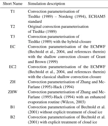
In Fig. 1 the seasonal cycle of the zonal average pre-cipitation is shown.
For all seasons the overall shape of the simulated precip-itation patterns agrees well with the observations, for exam-ple the maximum precipitation in the tropics, two secondary maxima in the Northern and Southern Hemispheric storm tracks, and minima in the subtropics and the polar regions.
However, the absolute values of the maxima differ signif-icantly, partly overestimating precipitation by up to 20%– 30% (T1, B2), whereas others capture the absolute value within ±5% (ZH, ZHW) or underestimate the observed max-imum by up to 20% (EC, EC2).
For boreal winter all simulations show a minimum in the Southern Hemisphere around 30◦S which is less distinct in the observations. The maximum in the tropics shows a double-peaked shape in the observations as well as in most of the simulations (not T1, ZH, ZHW). However, in the
ob-1info and data available from:http://disc.gsfc.nasa.gov/
data/datapool/TRMM DP/01 Data Products/02 Gridded/ 02 Monthly Pr Prod 3A 25/
Winter Spring
Summer Autumn
Fig. 1. Zonal average precipitation in mm/day for the four seasons (6 year average): for boreal winter (DJF), spring (MAM), summer (JJA)
and autumn (SON).
servations the southern peak is more pronounced, whereas in most of the simulations the Northern maximum is higher.
T1 significantly overestimates the maximum and it is much broader compared to most of the other simulations. The Northern Hemisphere is captured reasonably well with only small differences between the specific simulations.
For boreal spring again the largest differences occur in the tropics. While EC and EC2 both underestimate the absolute zonal average value, T1, T2, T3, B1, and B2 overestimate it, partly by more than 30%. ZH and ZHW perform best for the zonal average. Between 35◦N and 70◦N the simulated val-ues differ substantially, being higher than the observed valval-ues north of 40◦N. The EC, EC2, ZH and ZHW simulations fail to capture this secondary maximum in the Northern storm tracks at around 38◦N, though calculate it further north.
For boreal summer the differences are most pronounced, both in the tropics and in the extra-tropics. First, all simu-lations overestimate the secondary maximum in the southern
hemispheric storm tracks, and also in the Northern Hemi-sphere a similar feature occurs. The absolute values in the tropics are strongly overestimated by the Tiedtke and the Bechtold simulations. On the other hand the ECMWF scheme and the Zhang-McFarlane-Hack scheme tend to un-derestimate the maximum values in the ITCZ. Most simu-lations produce a precipitation peak around 30◦N. This is related to the steep orography of the Himalaya and the Ti-betan plateau, as can be seen in Fig. 2, for which the rainfall is substantially overestimated.
For boreal autumn the situation is similar to the spring. The southern storm tracks maximum is located too far north in all simulations, similar to that in the Northern Hemisphere. Another difference is that in most simulations (not T1 and ZHW) high precipitation values are calculated around 5◦S, which are not observed. T1 substantially overestimates the precipitation in the tropics.
GPCP T1
T2 T3
EC ZH
ZHW B2
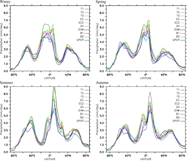
Fig. 2. Observed and simulated horizontal distribution of precipitation in mm/day (6 year average). The upper left panel shows the GPCP
Annual average
The observed and simulated annual average horizontal global precipitation distribution is analysed in Fig. 2. As indicated by Fig. 1 the main rainfall patterns are simulated in agreement with the observations. However, in some sim-ulations significant regional deviations from the observed values occur. Since the differences in the spatial distribution between EC and EC2, and B1 and B2, respectively, are small, only one of each group is shown here, namely EC and B2.
All simulations overestimate the precipitation over the continents in the tropics and in the southern storm tracks. Except for the EC simulations, all convection schemes have a severe problem in the Himalaya/Tibet region (mainly during summer, cf. Fig. 1). This has also been identified during the evaluation of the hydrological cycle of the ECHAM5 model (Hagemann et al., 2006) and has been associated with prob-lems arising from steep orography. A similar problem occurs over southern South America, where the steep mountains of Patagonia lead to a high simulated precipitation rate which is not observed.
And finally, all simulations underestimate precipitation in the central Atlantic ITCZ.
The small modifications of T1 compared to T2 and T3 re-sult in slightly different precipitation patterns. The regions with the largest deviations from the observations are simi-lar, i.e., a substantial overestimation of precipitation over the warm pool and the South Pacific Convergence Zone (SPCZ), west of the northern part of South America and in the con-tinental westward outflow into the Pacific ITCZ, over Cen-tral Africa, and Tibet. The large amount of precipitation in these regions leads to the overestimation in the zonal aver-ages shown in Fig. 1.
The largest overestimation in T1 is north and east of In-donesia, while in T2 and T3 it is shifted westward over land, although the precipitation over Thailand, Vietnam, etc. is un-derestimated.
In the Northern Hemispheric mid-latitudes the differences to the observations are only small in all Tiedtke simulations, except for the northern Pacific where T1 only slightly, but T2 and T3 significantly underestimate the average rainfall.
The differences between T1 and T2 can be related mainly to the different closure assumption (CAPE versus mois-ture convergence) and the different entrainment formula-tions. Most likely the different closure assumption causes the shifted precipitation patterns, since the entrainment for-mulation mainly affects the height of the convective clouds, whereas the closure determines the overall strength of the convective events. The other processes are identical between the T1 and T2 simulation.
The EC simulations are characterised by overall smaller differences to the observations. Some higher values occur in the Central Pacific (ITCZ, SPCZ), north of Madagascar, and in the southern storm tracks. Over the tropical
conti-nents the differences to the observations are small (positive in Central Africa, but negative in Indonesia and South Amer-ica). With EC, the total amount of simulated precipitation is much closer to the observed values in most regions, indicat-ing a better performance with respect to both, total amount and spatial distribution.
EC mainly differs from T1 with respect to the different trigger criterion, and the alternative description of the shal-low convection. Consequently these process descriptions likely explain the differences with T1. The shallow convec-tion in EC yields relatively strong mass fluxes (Tompkins et al., 2004), which originate from a slightly different for-mulation of the entrainment and result in a more effective mixing of the lower troposphere and less transport of mois-ture into the middle and upper troposphere. In contrast, the closure assumption and the microphysics are similar in EC and T.
The ZH simulation is characterised by the strongest dif-ferences compared to the observations, i.e., a large over-estimation over the tropical continents, especially Central Africa, the northern part of South America, India, and the Himalaya/Tibet region, and underestimation in parts of the tropical ITCZ over the ocean. Additionally, the simulated precipitation in the northern Pacific is less than observed, while it is slightly overestimated in Canada and the northern USA.
The ZHW simulation, in which an additional evaporation of convective precipitation in less cloudy areas is applied (Wilcox, 2003), leading to a better representation of the hy-drological cycle in the MATCH model (Lang and Lawrence, 2005a), results in a reduction of the overestimation over the continents compared to ZH. On the other hand, over the ocean the same adjustment results in stronger underestima-tion. In the mid-latitudes the differences are similar to those of the ZH simulation, since the “Wilcox (2003) adjustment” affects only the Zhang-McFarlane part of the convection pa-rameterisation which is mainly relevant for deep tropical convection, while the Hack part is more important in mid-latitude convection. In general it cannot be concluded that the precipitation distribution improves with this configura-tion compared to ZH.
The Bechtold simulations overall show an overestimation over, both, ocean and continents, most pronounced in the tropics, but also in the mid-latitudes. The patterns are captured very well, however with a global average positive bias. Similar to most other simulations precipitation is significantly overestimated in the Himalaya/Tibet region. Furthermore, in central Africa and east of the African coast too strong rainfall is calculated with this convection scheme. Statistical analysis
In addition to the differences of the annual average precipitation, some statistical analysis is performed
us-Table 3. Comparison of simulated and observed total precipitation rates and distributions (a) GPCP dataset, b) TRMM dataset, limited to
40◦S to 40◦N). The global mean observed GPCP precipitation flux is 2.62 mm/day, the observed convective precipitation flux from TRMM (40◦S to 40◦N) is 1.29 mm/day). For both, model and observations the mean values are area weighted. The root mean square error (RMSE) is calculated after the bias has been subtracted. R2is the correlation coefficient, the linear regression between model and observations is listed in terms of slope and intercept.
a) GPCP
– mean [mm/day] bias [mm/day] bias [%] RMSE [mm/day] R2 slope intercept
T1 3.00 0.38 14.5 1.52 0.70 1.13 –0.01 T2 2.91 0.29 11.0 1.43 0.69 1.07 0.05 T3 2.93 0.31 11.7 1.37 0.72 1.09 0.03 EC 2.87 0.25 9.5 1.11 0.72 0.90 0.40 EC2 2.86 0.24 9.0 1.12 0.70 0.88 0.45 ZH 2.82 0.20 7.6 1.52 0.57 0.87 0.42 ZHW 2.71 0.09 3.3 1.44 0.60 0.87 0.36 B1 3.14 0.52 19.8 1.32 0.68 0.98 0.43 B2 3.21 0.59 22.5 1.33 0.67 0.98 0.46
b) low resolution TRMM convective precipitation
– mean [mm/day] bias [mm/day] bias [%] RMSE [mm/day] R2 slope intercept
T1 2.13 0.84 65.2 3.84 0.71 1.93 –0.41 T2 2.46 1.17 90.9 3.27 0.78 2.16 –0.41 T3 2.46 1.17 90.7 3.14 0.78 2.16 –0.41 EC 2.40 1.12 86.7 2.43 0.72 1.54 0.36 EC2 2.48 1.19 92.5 2.48 0.69 1.57 0.39 ZH 3.00 1.71 132.7 3.14 0.61 1.79 0.64 ZHW 2.62 1.33 103.6 2.28 0.61 1.66 0.47 B1 2.61 1.33 103.1 2.27 0.72 1.83 0.20 B2 2.67 1.38 107.2 2.25 0.72 1.84 0.23
ing both observation datasets (GPCP and TRMM) for comparisons.
For GPCP (as already indicated in Fig. 1 and Fig. 2) all simulations show on average a higher total precipita-tion amount (as presented in Table 3a), with the relative bias being largest (22.5%) for the B2 simulation. The de-fault model setup still overestimates the precipitation rate by 14.5%, while the ZHW simulation is closest to the observa-tions with respect to the daily average rainfall.
The lowest de-biased root mean square error (RMSE) is found for the EC simulation, which also shows the highest correlation with the GPCP pattern. The slope of the linear regression is closest to unity for the Bechtold simulation, but the intercept shows a substantial offset. This confirms that the distribution is captured quite well with this model config-uration, but shows a systematic positive bias.
For the TRMM data the same statistics are calculated for the convective precipitation contribution of the model sim-ulations comparing with the convective precipitation of the 3A25 product (shown in Table 3b).
It is apparent, that all simulations substantially overesti-mate the convective precipitation in the region covered by the satellite data, some by more than 100% (ZH, ZHW, B1, B2), even T1 which is best with 65% overestimation. This overes-timation also results in very high RMSE values. The spatial patterns are represented comparable to the GPCP data, with T2 and T3 being correlated highest and ZH and ZHW show-ing the worst correlation. Due to the strong overestimation of the model results the slope is also too high.
The reason for this overestimation of the model results compared to the TRMM data can be determined from the fractionation into large-scale and convective precipitation, which is analysed in Table 4. In contrast to the TRMM data with a convective fraction of about 50% in the region cov-ered by the satellite, the simulated convective precipitation fraction varies between 62% (T1) and 95% (ZH). Most of the models setups calculate fractions of about 75% convec-tive contribution to the total precipitation.
The high values of the Zhang-McFarlane-Hack scheme seem unrealistic, although it must be considered that the
Table 4. Average fraction of large-scale and convective
precipita-tion for the different simulaprecipita-tions, limited from 40◦S to 40◦N. The convective precipitation fraction according to TRMM 3A25 data is 51.9% for the low resolution and 50.1% for the high resolution data.
Simulation Convective Large-scale Precipitation Precipitation Fraction [%] Fraction [%] T1 62.4 37.6 T2 75.4 24.6 T3 74.5 25.5 EC 75.5 24.5 EC2 78.1 21.9 ZH 95.0 4.5 ZHW 89.2 10.8 B1 74.1 25.9 B2 73.8 26.2
Hack part of the scheme is an adjustment scheme which tends to stabilise the atmosphere. Therefore, high humid-ity values can lead to instabilities and consequently trigger the convective adjustment which produces precipitation. For the large-scale cloud scheme this results in already reduced moisture and less precipitation formation in this model con-figuration. This can be understood in sight of the applied operator splitting technique, since the convection scheme is called before the large-scale cloud routines. In the simulation with the Bechtold scheme the convective fraction is similar to the T2 and T3 simulations and slightly lower than with the ECMWF scheme. Anyhow, it cannot be guaranteed that the TRMM retrieval algorithm for the distinction of large-scale and convective precipitation represents the reality perfectly.
A comparable analysis of total TRMM precipitation as for the GPCP data (as in Table 3) results in overestimated (be-tween 13 and 40%) rainfall and a slightly worse representa-tion (R2 between 0.46 and 0.75) of the spatial distribution (not shown in detail). This partly originates from the restric-tion to 40◦S to 40◦N, not taking the relatively good agree-ment of the simulated precipitation in the polar and subpolar regions into account.
4.1.2 Evaporation
Since there is no global evaporation dataset available due to its large heterogeneity, only the average values between the individual simulations are compared. Furthermore, the aver-age precipitation is compared with the averaver-age evaporation to close the hydrological cycle (Table 5).
For the T1 and T3 simulation the globally average annual evaporation completely balances the precipitation, for T2 al-most. Since the T1 model setup is ’tuned’ and the physical process descriptions between T2, T3 and T1 do not differ much, this is to be expected. The simulations with the EC scheme show a slightly higher evaporation than
precipita-Table 5. Mean evaporation and precipitation fluxes for the various
simulations.
Simulation Evaporation Precipitation
mean mean [mm/day] [mm/day] T1 3.00 3.00 T2 2.90 2.91 T3 2.93 2.93 EC 2.94 2.87 EC2 2.91 2.86 ZH 2.83 2.82 ZHW 2.68 2.71 B1 2.95 3.14 B2 3.05 3.21
tion. However, a time series analysis of the soil moisture and the specific humidity shows no drift into a higher or lower regime, and also it is not an issue caused by the model spin-up. Consequently, the enhanced evaporation occurs over the quasi-unlimited moisture reservoir of the oceans. As in the Tiedtke simulations, in the ZH and ZHW model config-urations a near-balance is calculated, while in the simula-tions using the Bechtold scheme the calculated precipitation is substantially higher than the evaporation. For the latter scheme this can result from a modification of the scheme as applied in this study. In the original scheme it is checked whether the mass of water within the column is conserved before and after the call of the convection scheme, and in case of a difference the difference is uniformly distributed over all levels. However, in the stratosphere with very low values of humidity this is not applicable. Therefore, it is not the humidity, but the precipitation flux which is adjusted in this model configuration. Consequently the discrepancies between evaporation and precipitation result from a weak-ness of the scheme, i.e. it is not fully water mass conserving. Therefore, the results of the EC and B simulations must be analysed with care, and this imbalance may lead to runaway drying or moistening of specific regions. However, in none of the simulations such a feature occurs within the six years of the simulation period. Since these convection schemes are both applied in weather prediction models, less emphasise is given in the schemes to mass conservation, since they are applied only for limited time periods.
4.1.3 Water vapour content of the atmosphere
Since a detailed analysis of the three-dimensional water vapour distribution is beyond the scope of this study, only the total water vapour content (i.e., the integrated water vapour column (IWVC)) of the atmosphere is compared to observa-tions. Furthermore, a comparison of the zonal average water vapour between five simulations is shown for the upper tro-posphere - lower stratosphere (UTLS) region.
Winter Summer
Fig. 3. Zonal average integrated water vapour column in cm for boreal winter (DJF) and summer (JJA) (5 year average).
Observational dataset
The global dataset of the IWVC originates from com-bined measurements of GOME and SSM/I, presented by Lang and Lawrence (2005a,b). It starts in August 1995, therefore, only data from January 1996 to December 2000 (5 years also fully covered by the simulation period) are used for the analysis.
IWVC zonal average
As can be seen in Fig. 3 the overall shape of the zonal average IWVC agrees very well with the observations in all simulations.
On both hemispheres the gradient towards the equator is very similar. In boreal winter the absolute values in the trop-ics are higher than the observations in the EC, EC2, and ZHW simulation, while T1, T2, and T3 capture the maxi-mum correctly. ZH, B1, and B2 all underestimate the abso-lute value in the tropics and show consequently a less steep gradient towards the equator. Around 40◦N the observed IWVC is lower than the simulated in all setups.
In boreal summer the shape is very similar for all sim-ulations in the tropics, again with some overestimation in T1, T3, ZHW, EC, EC2, and underestimation in ZH, B2 of ±0.5 cm around the maximum observed value. In the extra-tropics more significant discrepancies occur. None of the convection schemes reproduces the observed low values around 40◦S, and the overestimation at these latitudes ex-ceeds 30% for all schemes. In the Northern Hemisphere a slightly enhanced IWVC is simulated by all schemes around 40◦N, which does not occur in the observations. Even though this feature also appears in the ZH and B2 simula-tions the absolute values are lower than the observed south of 40◦N.
In addition, all schemes overestimate the IWVC between 50◦N and 65◦N, with ZHW being worst with an overestima-tion of about 30%.
Overall the zonal structure is captured quite accurately by all model simulations.
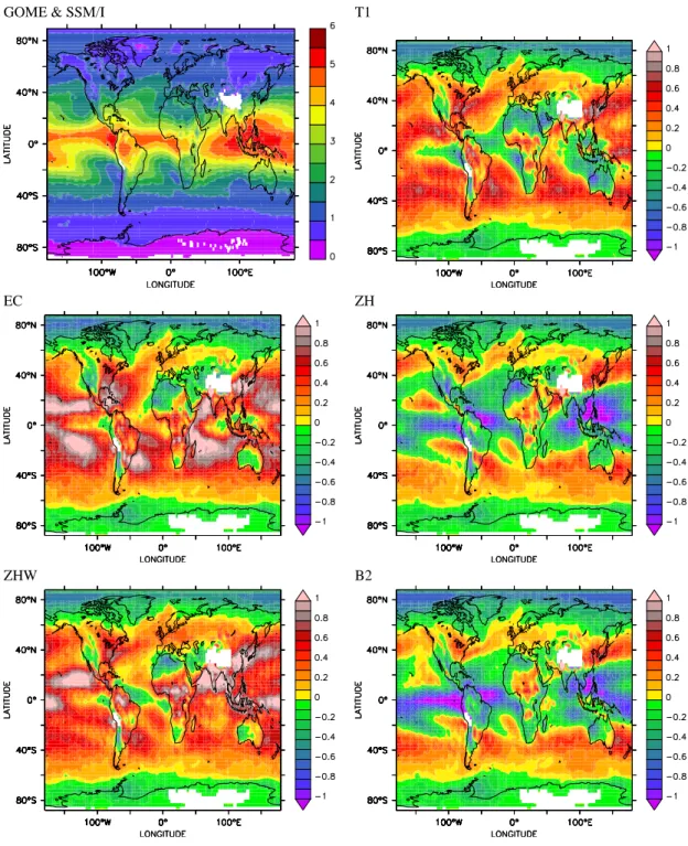
IWVC annual average
The spatial patterns of the IWVC are depicted in Fig. 4. The observations (upper left panel) show highest water vapour columns in the tropical ITCZ with maxima over the warm pool and at the northern coast of South America. The meridional gradient is steeper from the equator up to 40◦ than further poleward. The subsidence regions of the subtropics are characterised by relatively low water vapour. Even though substantial evaporation takes place in these regions the water is transported towards the equator at low altitude in the Hadley circulation (e.g. Trenberth and Stepaniak, 2003), while subsidence suppresses deep convection and substantial upward transport of moisture.
The T1 simulation shows lower values in most oceanic parts of the ITCZ and the Sahara, while almost everywhere in the mid-latitudes higher values than observed are calcu-lated. This indicates that the model does not accurately cap-ture the meridional gradients. The underestimated IWVC in the tropics is partly consistent with regions of high precipita-tion (cf. Fig. 2), e.g., west of tropical South America precip-itation is overestimated, and the atmospheric water vapour content is underestimated. However, this does not hold in general, since over the Atlantic ITCZ both IWVC and pre-cipitation are underestimated. Over the warm pool the IWVC is overestimated, too, possibly resulting from too high evap-oration leading to overestimated atmospheric moisture and rainfall in this region.
GOME & SSM/I T1
EC ZH
ZHW B2
Fig. 4. Horizontal distribution of the annual average (5 years) IWVC in cm. The upper left panel shows the observed values, while the others
depict the differences between the individual simulations and the observations (model minus observations) in cm. White areas are regions for which no observations are available.
The EC simulation shows many regions in which sub-stantially higher IWVC values are calculated, mainly in ma-rine environments where convection is active (ITCZ, SPCZ, Caribbean, Indian Ocean). Again, this is consistent since in these regions the precipitation is much lower with this con-vection parameterisation compared to the Tiedtke scheme.
Since moisture is transported from the evaporation regions in the subtropics into the convergence zones and does not pro-duce precipitation as efficiently in EC compared to T1, the simulated IWVC is higher. Over the continents the differ-ences are relatively smaller, except for the rain forest regions of Africa and South America.
Table 6. Comparison of the simulated and observed (GOME&SSM/I) IWVC values and distributions. The mean observed vertically
integrated water vapour column is 2.33 cm. For both model and observations the mean values are area weighted. The root mean square error (RMSE) is calculated after the bias has been subtracted. R2is the correlation coefficient, the linear regression between model and observations is listed in terms of slope and intercept.
– mean [cm] bias [cm] bias [%] RMSE [cm] R2 slope intercept
T1 2.51 0.17 7.4 0.30 0.94 1.01 0.13 T2 2.44 0.11 4.8 0.28 0.94 0.97 0.16 T3 2.48 0.15 6.3 0.27 0.94 0.99 0.14 EC 2.66 0.33 14.2 0.36 0.94 1.09 0.09 EC2 2.62 0.28 12.2 0.33 0.94 1.07 0.08 ZH 2.26 –0.07 –3.0 0.35 0.91 0.86 0.23 ZHW 2.67 0.34 14.4 0.31 0.95 1.09 0.10 B1 2.31 –0.02 –0.7 0.33 0.93 0.90 0.19 B2 2.25 –0.09 –3.7 0.35 0.92 0.87 0.19
In the simulation with the ZH convection parameterisation significantly lower IWVC values are calculated in the trop-ics, with the exception of Central Africa. These are mostly regions where the precipitation (Fig. 2) is captured accurately or slightly underestimated. In the mid-latitude storm tracks higher moisture is simulated than observed.
In the ZHW simulation with the enhanced evaporation the integrated water vapour column reaches much higher values in the tropics, overestimating the observations significantly. The meridional gradient is comparable to the measurements. Consequently, the absolute values are also too high in the mid-latitudes.
The B2 simulation (lower left panel in Fig. 4) shows an underestimation of column water vapour in the tropics and an overestimation in the mid-latitudes. In the tropics this is again consistent, since precipitation is strongly overes-timated (cf. Fig. 2) in these regions. Even though in the mid-latitudes the IWVC is also overestimated, this argument is not applicable there, since the precipitation is also too strong. Therefore, this indicates that either the evaporation is too high in these regions or the poleward transport of moisture from the subtropics into the storm tracks is too rapid in this setup.
IWVC statistical analysis
A statistical summary of the comparison with obser-vations is presented in Table 6. The mean values and corresponding biases show that in some simulations the global average IWVC is overestimated, notably in those using the Tiedtke, ECMWF and ZHW schemes, whereas the ZH and Bechtold simulations underestimate the vertical water vapour column. However, only the EC simulations and ZHW have a bias larger than 10%. The lowest global average bias is found for the B1 simulation. Comparison of the horizontal patterns, using the de-biased RMSE as indicators, shows that the T3 simulation best represents the
observed patterns. Nevertheless, the results for all other tested setups are similar. All simulated patterns are highly correlated to the observed distribution with correlation coefficients R2ranging from 0.91 (ZH) to 0.95 (ZHW). This is also confirmed by the slopes of the linear regression being close to one.
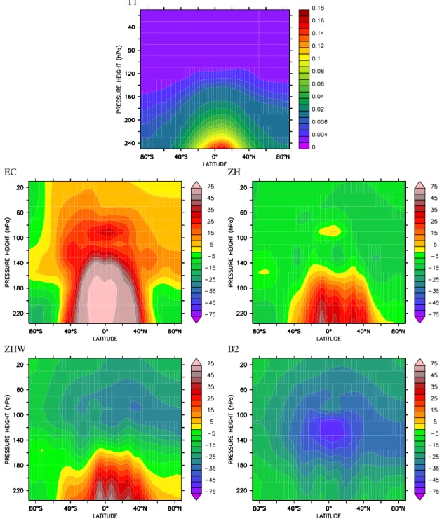
Water vapour in the UTLS
Convection is a key process that moistens the upper troposphere - lower stratosphere (UTLS) region. Depending on the convection scheme, the amount of total water is reduced by precipitation partly balancing the moistening process. Differences in water vapour in the upper tropo-sphere can result from both different convective transport strength and drying efficiency.
To identify these effects the specific humidity above 250 hPa is shown in Fig. 5. The results of the T1 simulation (used as a reference for this analysis and depicted in the up-per panel) show the typical distribution, with highest values in the tropics and a strong gradient across the tropopause. Note that detailed features of the water vapour distribution like the tape recorder and the quasi-biennial oscillation can-not be simulated due to the relatively coarse vertical resolu-tion in the UTLS in the chosen model configuraresolu-tion with 31 layers up to 10 hPa.
In the EC simulation substantially more (>75%) water vapour is transported into the tropical upper troposphere. Since the convection scheme is the only difference with the reference simulation, this must be a direct or indirect sequence of convection. Due to higher moisture at the con-vective cloud tops, more water vapour enters the stratosphere having an impact on radiative cooling and consequently the temperature and the dynamics. At high latitudes the differ-ences are of opposite sign, but are substantially smaller.
The ZH simulation similarly computes more water vapour in the upper troposphere, but less than EC. Moreover, the
T1
EC ZH
ZHW B2
Fig. 5. Zonal average specific humidity (6 year average) above 250 hPa. The upper panel shows the zonal distribution from the T1 reference
simulation in gwater/kgair. The other panels depict the relative differences in % to this reference.
higher values do not reach as high, leading only to slightly more moisture in the stratosphere. Therefore, the influence of replacing the Tiedtke by the Zhang-MacFarlane-Hack con-vection schemes is largely limited to the troposphere.
This is also valid for the ZHW simulation. In contrast to EC and ZH, ZHW humidity is somewhat higher compared to T1 also in the polar regions. Additionally, in the strato-sphere of the Northern Hemistrato-sphere lower specific humidity is computed.
The simulation B2 shows values comparable to T1 in the upper troposphere, but substantially lower values between 140 and 100 hPa at low latitudes. In contrast to the other convection schemes, less water is transported into the upper troposphere and reaches the stratosphere.
The effects of the different convection schemes are consistent with the results discussed above. The EC scheme produces less precipitation than the reference T1. Conse-quently more moisture is transported into the UTLS region.
Fig. 6. Taylor diagram for the global precipitation (crosses) and
water vapour column (triangles). The standard deviation of the model calculations is normalised with the observed standard devia-tion. The various simulations are indicated by different colours.
The same is valid for ZH and ZHW. B2 produces even more precipitation than T1, and as a consequence less water can be transported upward and enter the stratosphere. The water vapour content of the UTLS has a strong impact on temper-ature, the tropopause structure and stratosphere-troposphere exchange processes.
Summary
Figure 6 summarises the comparisons with observa-tions in a Taylor diagram (Taylor, 2001) for which all quantities have been normalised to the observed standard deviation. The precipitation, denoted by the crosses, shows the highest correlation and the normalised standard deviation (σ ) closest to unity for the EC simulation. Therefore, the spatial patterns of the average precipitation are overall captured best. The other simulations are slightly worse, e.g., B1 and B2 are less strongly correlated to the observations, but σ is closer to 1 compared to the Tiedtke simulations. For the ZH simulations the correlation is lower. The best representation of both, spatial distribution and absolute values is achieved with the ECMWF scheme. For the IWVC the results are summarised by the triangles. The correlation is high for all simulations and the amplitude of the spatial and temporal variation is also well reproduced (best for B1, but only slightly worse for the other schemes).
Figure 6 shows that the patterns of the IWVC are captured much better than the precipitation patterns. Additionally, it indicates that the simulated IWVC is more robust in view of
replacing the convection scheme than the precipitation. Nev-ertheless, both quantities are substantially influenced by the parameterisation. A scheme that performs best with respect to both the precipitation and the IWVC cannot be identified, especially if the bias is additionally taken into account. As seen in Fig. 3 and Fig. 4, the overall spatial patterns are sim-ulated relatively accurately by all model configurations with each scheme having some weaknesses.
Furthermore, the effect of the different convection schemes on the UTLS region is substantial.
4.2 Global meteorology
The selected convection scheme has a direct impact on the simulated climate. As shown above, the hydrological cycle is substantially modified by exchanging the convection pa-rameterisation. Due to the influence of clouds, water vapour, etc. on radiation, changes in the energy budget are to be ex-pected. Since the model system in the T1 configuration is the default for ECHAM5 and has been “tuned” to reproduce present-day climate (Roeckner et al., 2006), the T1 simula-tion is taken as reference for this secsimula-tion.
As shown in the section above, the water vapour distribu-tion is substantially modified by the exchange of the convec-tion scheme. Via the feedback mechanisms in the climate model this has effects on large-scale cloud formation, the ra-diation fluxes, etc. in a way that this tuning is probably not valid in the altered model configurations.
4.2.1 Energy budgets
The energy fluxes at the surface simulated by the individ-ual model configurations are compared in Table 7. None of the simulations show a trend in the global average energy fluxes over the simulation period. Therefore, a stable model climate has been achieved in all cases, which indicates the physical consistency of the ECHAM5 model, but it cannot be stated that is also the case for longer integration periods. For such studies a “re-tuning” of the model setup might be required. The simulations can be classified into two groups: The Tiedtke and the Zhang-McFarlane-Hack simulations are close to each other with respect to the solar and infrared ra-diation at the surface. Since the evaporation is smaller with the Zhang-McFarlane-Hack scheme, consequently the latent heat flux is reduced and the sensible heat flux is larger com-pared to the Tiedtke simulations.
The other group consists of the ECMWF and the Bechtold simulations. Both compute significantly lower solar radia-tion fluxes at the surface. The IWVC for the EC simularadia-tion (compare Fig. 4) in the tropics is higher than observed and than in the reference simulation (T1), resulting in a more ef-fective short wave radiation absorption, and stronger cloud formation leading to higher reflectance. Furthermore, as seen in Fig. 5 with EC, there is much more water vapour in the up-per troposphere contributing to radiative cooling.
Table 7. Energy budget of the atmosphere at the surface. All fluxes are area weighted 6 year averages. The unit is W/m2. The net solar radiation and the net thermal radiation are calculated by the radiation module, the latent heat flux is the evaporation multiplied with the latent heat of vaporisation (L). The residual sensible heat flux is calculated assuming a closed energy budget. Furthermore, the computed thermal radiation at the top of the atmosphere is presented.
Simulation Net solar radiation Net thermal radiation Latent heat flux Sensible heat flux Thermal radiation at the surface at the surface (L * evaporation) (residual) top of the atmosphere
T1 167.9 –55.96 –86.92 –25.02 –235.0 T2 171.3 –57.24 –84.10 –29.94 –233.2 T3 171.2 –57.07 –84.74 –29.41 –233.5 EC 150.8 –50.20 –85.13 –15.51 –232.3 EC2 149.7 –49.63 –84.25 –15.81 –232.0 ZH 178.1 –61.87 –81.88 –34.32 –233.7 ZHW 169.1 –57.97 –77.56 –33.61 –227.1 B1 152.5 –50.13 –85.46 –16.94 –231.5 B2 157.1 –51.62 –88.49 –16.99 –236.5
For the B2 simulation there is neither higher IWVC in the tropics nor higher water vapour in the UTLS. Nevertheless, the different trigger conditions and microphysical scheme of this convection parameterisation can lead to stronger cloud formation, which also reduces the net solar radiation flux at the surface. Even though the global surface temperature does not deviate strongly from the reference simulation (see below), the net infrared radiation flux in B2 is smaller by several W/m2than in the reference.
For all simulations the latent heat flux reflects the differ-ences in evaporation.
Since the differences in the solar radiation at the surface are much larger than those in the thermal radiation, the resid-ual sensible heat flux is much reduced in the simulations of the second group. This likely influences the development of the convective boundary layer.
An important parameter indicating climate change is the outgoing long-wave radiation (OLR) at the top of the atmo-sphere. The average values for the individual simulations are presented in the last column of Table 7. Taking the value of the “tuned” T1 model configuration as a reference (in Wild and Roeckner (2006) exactly the same value is given for the OLR), the other Tiedtke simulations already deviate by more than −1.5 W/m2. The simulations with the EC scheme result in even lower values by almost −3 W/m2. The ZH simula-tion yields lower deviasimula-tions than the T3 simulasimula-tions indicat-ing the smallest deviation from present-day conditions. The low value of the ZHW simulation shows a strong variation of the OLR, being significantly too low. The B1 simulation results also in too low values, being lower than the EC config-urations. On the other hand, the B2 simulation shows even larger OLR average values. Compared with the references by observed data, given in Wild and Roeckner (2006), this higher value is also quite realistic.
In summary, although there are some differences in the energy budgets all simulations produce stable, slightly
differ-ent states of the atmosphere. In comparison with the evalua-tion of the radiaevalua-tion fluxes in the standard ECHAM5 model (Wild and Roeckner, 2006) with satellite data, the short-wave fluxes of the first group are more realistic for present day con-ditions. However, the thermal radiation at the top of the at-mosphere appears quite realistic in the B2 simulation, while the other simulations deviate partly significantly from the ref-erence simulation (−7.9 W to +1.5 W).
4.2.2 Effects on temperature
The effects on the temperature distribution are illustrated in Fig. 7, which shows the correlation of the temperature be-tween the individual simulations and the reference simula-tion T1. The correlasimula-tion is very high and the linear regres-sion is very close to the one-to-one line for all simulations. However, the scatter indicates differences by several degrees in the region of the highest temperatures (lower troposphere). In the upper troposphere the range is even broader, indicat-ing variations of ±10 K. This can partly be attributed to the modified water vapour content in the UTLS region, where the temperature is highly sensitive to absorption and re-emission of radiation.
However, the symbols do not show any specific tendency to over- or underestimate the temperature relative to the ref-erence in neither the upper, the middle, nor in the lower at-mosphere. This indicates that the temperature structure of the atmosphere is not significantly altered by exchanging the convection parameterisation.
Finally, the global average temperatures are compared in Table 8.
The global average temperature of the atmosphere (up to 10 hPa) simulated with the individual convection schemes is within ±0.8 K of the reference simulation. The highest value results from the EC, the lowest from the B2 simulation. The simulations with the ZH scheme show only minor changes of the global average temperature of the atmosphere.
T1 ⊲⊳ EC T1 ⊲⊳ ZH
T1 ⊲⊳ ZHW T1 ⊲⊳ B2
Fig. 7. Temperature correlation between the reference simulation (T1) on the horizontal axis and the individual simulations (EC, ZH, ZHW
and B2) on the vertical axis, colour coded with pressure altitude. The monthly average temperatures of the evaluated time series have been transformed onto a 10◦×10◦grid. The black line depicts the one-to-one line.
Table 8. Statistics of the simulated temperature with T1 as a
ref-erence. Column 1 and 2 list the horizontally area weighted and vertically unweighted 6 year 3-D averages; column 3 and 4 show the 2-D area weighted 6 years averages.
atmosphere (up to 10 hPa) surface layer
Simulation Mean Bias Mean Bias
Name [K] [K] [K] [K] T1 245.8 – 287.3 – T2 245.6 –0.14 287.2 –0.10 T3 245.9 0.11 287.3 –0.00 EC 246.6 0.79 287.0 –0.30 EC2 246.2 0.46 286.8 –0.49 ZH 246.0 0.27 287.0 –0.26 ZHW 246.1 0.30 287.1 –0.19 B1 245.3 –0.50 286.9 –0.40 B2 245.0 –0.78 286.6 –0.66
The temperature in the lowest model layer shows on aver-age lower values for the EC and Bechtold simulations, since the net solar radiation is reduced. However, the relative tem-perature deviations from the reference are much smaller than
the relative differences in the incoming short wave radia-tion, which are consistently balanced by other processes, e.g., through the boundary layer meteorology. The average sur-face temperature for the ZH scheme is also slightly lower than in the reference simulation. In addition to the radiation effects the altered hydrological cycle has an impact on the temperature in the lowest model level via changed precipita-tion and evaporaprecipita-tion. Since this induces feedback processes with soil temperature and moisture, and boundary layer me-teorology, a direct assessment of all the processes involved is difficult. Even though the deviation from the reference is mainly small on the global average (<0.66 K), local dif-ferences can be much larger (up to ±5 K), as indicated by the range of the distributions in Fig. 7. This is directly sup-ported by the differences of the temperature in the surface layer between the individual simulations and the reference (not shown).
These global average differences are of the same magni-tude as temperature changes resulting from perturbed atmo-spheric conditions as applied in climate scenario calculations and the observed temperature change within the 20th cen-tury. Even though a direct comparison is not applicable, this indicates that the uncertainty resulting from different
formu-lations of the process description of subgrid-scale convection is still relatively large and is partly overcome by “model tun-ing”. However, no study of the behaviour of the individual model configurations under specified conditions have been performed to directly address the influence in climate sce-nario simulations.
5 Conclusions
Considering that convection plays a key role in the redistri-bution of heat, momentum and moisture in the atmosphere, it may be expected that the results of different convection schemes substantially impact the simulated weather, hydro-logical cycle and climate of a GCM. Our inter-comparison of four different convection parameterisations in ECHAM5, including several different versions and updates, neverthe-less shows that the results of all schemes are robust, i.e. the simulated meteorology is stable and realistic over the 6-year period considered. Although all parameterisations involved are mass-flux schemes, based on the original assumptions of modifying the moist static energy and humidity through in-teractions between convective cells and the large-scale envi-ronment (Arakawa and Schubert, 1974), they differ in impor-tant aspects about the triggering of convection, the closure assumption, and formulation of the cloud processes (e.g., en-trainment and precipitation formation).
The differences are generally not very large, especially in the zonal mean, and the computed water vapour columns are close to observations. Overall, the default ECHAM5 con-vection scheme T1 by Tiedtke (1989), with modifications by Nordeng (1994), simulates very realistic water vapour distri-butions, which is crucial for radiative transfer processes and atmospheric chemistry.
The alternative schemes give rise to somewhat larger dis-crepancies with observations, although the differences are mostly within about ±15%, probably close to or within the uncertainty range of the measurement climatology used. The differences are largest and partly quite significant for the UTLS region, especially in low latitudes, related to the depth of convection and the efficiency of precipitation formation.
The results of the inter-comparison for precipitation show larger differences and discrepancies compared to observa-tions. Both the absolute values and the spatial distribution of annual rainfall rates are best reproduced with the ECMWF convection scheme. Except ZHW all schemes seem to over-estimate precipitation in the ITCZ, over the Pacific warm pool and near strongly pronounced surface topography, the latter being treated most realistically by the EC scheme. Dis-crepancies are particularly significant for computed convec-tion over the Tibetan Plateau and the Andes mountain range. We have also considered some global characteristics of the atmospheric energy and moisture budgets. Some schemes, notably EC and B, appear to produce too much cloudiness, preventing solar radiation to reach the surface. As a
conse-quence, the outgoing IR radiation at the surface and the sensi-ble heat flux seem too low. Nevertheless, the effect on atmo-spheric temperature is generally small, on average ±0.8 K, although locally differences of ±5 K can occur, especially near the surface and upper troposphere.
Since all schemes have particular aspects for which they perform comparatively well or less well, it cannot unequivo-cally be concluded which of the schemes is superior. There-fore, we have no incentive to replace the T1 parameterisation as the standard convection scheme, although the triggering and depth of convection and the formation of precipitation may be further optimised. However, for specific studies over shorter time periods in which a better representation of the hydrological cycle might result in substantial improvements for the local meteorology such an exchange is probably use-ful.
Acknowledgements. We are grateful to P. Bechtold for providing
the code for the ECMWF and his own convection scheme. Fur-thermore we thank M. Lawrence for providing the MATCH-MPIC version of the Zhang-McFarlane-Hack scheme and the fruitful discussions and help with the code implementation. Additionally, we thank A. Bott for the supervision of the PhD thesis of H. Tost on which this paper is based. We acknowledge the work of R. Lang and thank him for providing the dataset with the IWVC observations, as well as the colleagues of the GPCP project for their datasets. Furthermore, we wish to acknowledge use of the Ferret program for analysis and graphics in this paper. Ferret is a product of NOAA’s Pacific Marine Environmental Laboratory. (Information is available at http://ferret.pmel.noaa.gov/Ferret/). Additionally we thank all MESSy developers and users for support and discussions.
Edited by: M. Dameris
References
Adler, R. F., Huffman, G. J., Chang, A., Ferraro, R., Xie, P., Janowiak, J. E., Rudolf, B., Schneider, U., Curtis, S., Bolvin, D., Gruber, A., Susskind, J., Arkin, P., and Nelkin, E.: The Version-2 Global Precipitation Climatology Project (GPCP) Monthly Precipitation Analysis (1979–Present), J. Hydrometeorology, 4, 1147–1167, 2003.
Arakawa, A.: The Cumulus Parameterization Problem: Past, Present, and Future, J. Clim., 17, 2493–2525, 2004.
Arakawa, A. and Schubert, W. H.: Interaction of a Cumulus Cloud Ensemble with the Large-Scale Environment, Part I, J. Atmos. Sci., 31, 674–701, 1974.
Bechtold, P., Bazile, E., Guichard, F., Mascart, P., and Richard, E.: A mass-flux convection scheme for regional and global models, Q. J. R. Meteorol. Soc., 127, 869–886, 2001.
Bechtold, P., Chaboureau, J.-P., Beljaars, A., Betts, A. K., K¨ohler, M., Miller, M., and Redelsperger, J.-L.: The simulation of the diurnal cycle of convective precipitation over land in a global model, Q. J. R. Meteorol. Soc., 130, 3119–3137, 2004.
Donner, L. J., Seman, C. J., Hemler, R. S., and Fan, S.: A Cumu-lus Parameterization Including Mass Fluxes, Convective Verti-cal Velocities, and MesosVerti-cale Effects: Thermodynamic and
Hy-drological Aspects in a General Circulation Model, J. Clim., 14, 3444–3463, 2001.
Emanuel, K. A. and Zivkovic-Rothman, M.: Development and Evaluation of a Convection Scheme for Use in Climate Models, J. Atmos. Sci., 56, 1766–1782, 1999.
Ghan, S., Randall, D., Xu, K.-M., Cederwall, R., Cripe, D., Hack, J., Iacobellis, S., Klein, S., Krueger, S., Lohmann, U., Pedretti, J., Robock, A., Rotstayn, L., Somerville, R., Stenchikov, G., Sud, Y., Walker, G., Xie, S., Yio, J., and Zhang, M.: A comparison of single column model simulations of summertime midlatitude continental convection, J. Geophys. Res., 105, 2091–2124, 2000. Grabowski, W. W.: An Improved Framework for
Superparameteri-zation, J. Atmos. Sci., 61, 1940–1952, 2004.
Grabowski, W. W. and Smolarkiewicz, P. K.: CRCP: a Cloud Re-solving Convection Parameterization for modeling the tropical convecting atmosphere, Physica, 133D, 171–178, 1999. Grant, A. L. M. and Brown, A. R.: A similarity hypothesis for
shallow-cumulus transports, Q. J. R. Meteorol. Soc., 125, 1913– 1936, 1999.
Grassl, H., Jost, V., Schulz, J., Kumar, M. R. R., Bauer, P., and Schluessel, P.: The Hamburg Ocean-Atmosphere Parameters and Fluxes from Satellite Data (HOAPS): A climatological Atlas of Satellite-Derived Air-Sea Interaction Parameters over the World Oceans, Tech. Rep. 312, Max-Planck-Institut f¨ur Meteorologie, 2000.
Hack, J. J.: Parameterization of moist convection in the National Center for Atmospheric Research community climate model (CCM2), J. Geophys. Res., 99, 5551–5568, 1994.
Hagemann, S., Arpe, K., and Roeckner, E.: Evaluation of the hydro-logical cycle in the ECHAM5 model, J. Clim., 19, 3810–3827, 2006.
Houze, jr., R. A.: Mesoscale Convective Systems, Rev. Geophys., 42, RG4003, doi:8755-1209/2004RG000150, 2004.
Huffman, G. J., Adler, R. F., Arkin, P., Chang, A., Ferraro, R., Gru-ber, A., Janowiak, J., McNab, A., Rudolf, B., and Schneider, U.: The Global Precipitation Climatology Project (GPCP) Combined Precipitation Dataset, Bull. Amer. Meteor. Soc., 78, 5–20, 1997. Jakob, C. and Siebesma, A. P.: A New Subcloud Model for Mass-Flux Convection Schemes: Influence on Triggering, Updraft Properties, and Model Climate, Mon. Wea. Rev., 131, 2765– 2778, 2003.
J¨ockel, P., Sander, R., Kerkweg, A., Tost, H., and Lelieveld, J.: Technical Note: The Modular Earth Submodel System (MESSy) — a new approach towards Earth System Modeling, Atmos. Chem. Phys., 5, 433–444, 2005,
http://www.atmos-chem-phys.net/5/433/2005/.
J¨ockel, P., Tost, H., Pozzer, A., Br¨uhl, C., Buchholz, J., Ganzeveld, L., Hoor, P., Kerkweg, A., Lawrence, M. G., Sander, R., Steil, B., Stiller, G., Tanarhte, M., Taraborrelli, D., van Aardenne, J., and Lelieveld, J.: The atmospheric chemistry general circulation model ECHAM5/MESSy1: consistent simulation of ozone from the surface to the mesosphere, Atmos. Chem. Phys., 6, 5067– 5104, 2006,
http://www.atmos-chem-phys.net/6/5067/2006/.
Kummerow, C., Simpson, J., Thiele, O., Barnes, W., Chang, A. T. C., Stocker, E., Adler, R. F., Hou, A., Kakar, R., Wentz, F., Ashcroft, P., Kozu, T., Hong, Y., Okamoto, K., Iguchi, T., Kuroiwa, H., Im, E., Haddad, Z., Huffman, G., Ferrier, B., Ol-son, W. S., Zipser, E., smith, E. A., wilheit, T. T., North, G.,
Krishnamurti, T., and Nakamura, K.: The Status of the Tropical Rainfall Measuring Mission (TRMM) after tow years in orbit, J. Appl. Meteorol., 39, 1965–1982, 2000.
Kuo, H. L.: Further Studies of the Parameterization of the Influence of Cumulus Convection on Large-Scale Flow, J. Atmos. Sci., 31, 1232–1240, 1974.
Lang, R. and Lawrence, M. G.: Improvement of the vertical hu-midity distribution in the chemistry-transport model MATCH through increased evaporation of convective precipitation, Geo-phys. Res. Lett., 32, L17 812, doi:10.1029/2005GL023172, 2005a.
Lang, R. and Lawrence, M. G.: Evaluation of the hydrological cycle of MATCH driven by NCEP reanalysis data: comparison with GOME water vapor measurements, Atmos. Chem. Phys., 5, 887– 908, 2005b.
Lawrence, M. G., Crutzen, P. J., Rasch, P. J., Eaton, B. E., and Mahowald, N. M.: A model for studies of tropospheric chem-istry: Description, global distributions and evaluation, J. Geo-phys. Res., 104, 26 245–26 277, 1999.
Lee, M.-I., Kang, I.-S., and Mapes, B. E.: Impacts of Cumulus Con-vection Parameterization on Aqua-planet AGCM Simulations of Tropical Intraseasonal Variability, J. Met. Soc. Japan, 81, 963– 992, 2003.
Lin, J. W.-B. and Neelin, J. D.: Considerations for Stochastic Con-vective Parameterization, J. Atmos. Sci., 59, 959–975, 2002. Lin, S.-J. and Rood, R.: Multidimensional Flux-Form
Semi-Lagrangian Transport Schemes, Mon. Wea. Rev., 124, 2046– 2070, 1996.
Lohmann, U. and Roeckner, E.: Design and performance of a new cloud microphysics scheme developed for the ECHAM general circulation model, Clim. Dyn., 12, 557–572, 1996.
Mahowald, N. M., Rasch, P. J., Eaton, B. E., Whittlestome, S., and Prinn, R. G.: Transport of222radon to the remote troposphere using the Modell of Atmospheric Transport and Chemistry and assimilated winds from ECMWF and the National Center for En-vironmental Prediction/NCAR, J. Geophys. Res., 102, 28 139– 28 151, 1997.
Masunaga, H., Nakajima, T. Y., Nakajima, T., Kachi, M., Oki, R., and Kuroda, S.: Physical properties of maritime low clouds as retrieved by combined use of Tropical Rainfall Measurement Mission Microwave Imager and Visible/infrared Scanner: Algo-rithm, J. Geophys. Res., 107, 4083, doi:10.1029/2001JD000743, 2002a.
Masunaga, H., Nakajima, T. Y., Nakajima, T., Kachi, M., and Suzuki, K.: Physical properties of maritime low clouds as re-trieved by combined use of Tropical Rainfall Measurement Mis-sion (TRMM) Microwave Imager and Visible/infrared Scanner: 2. Climatology of warm clouds and rain, J. Geophys. Res., 107, 4367, doi:10.1029/2001JD001269, 2002b.
Mori, S., Jun-Ichi, H., Tauhid, Y. I., Yamanaka, M. D., Okamoto, N., Murata, F., Sakurai, N., Hashiguchi, H., and Sribimawati, T.: Diurnal Land-Sea Rainfall Peak Migration over Sumatera Island, Indonesian Maritime Continent, Observed by TRMM Satelitte and Intensive Rawinsonde Soundings, Mon. Wea. Rev., 132, 2021–2039, 2004.
Negri, A. J., Bell, T. L., and Xu, L.: Sampling of the Diurnal Cycle of Precipitation using TRMM, J. Atmos. Ocean Tech., 19, 1333– 1344, 2002.