HAL Id: hal-02001498
https://hal.uca.fr/hal-02001498
Submitted on 31 Jan 2019
HAL is a multi-disciplinary open access
archive for the deposit and dissemination of
sci-entific research documents, whether they are
pub-lished or not. The documents may come from
teaching and research institutions in France or
abroad, or from public or private research centers.
L’archive ouverte pluridisciplinaire HAL, est
destinée au dépôt et à la diffusion de documents
scientifiques de niveau recherche, publiés ou non,
émanant des établissements d’enseignement et de
recherche français ou étrangers, des laboratoires
publics ou privés.
PiRAT: Pivot Routing for Alarm Transmission in
Wireless Sensor Networks
Nancy Rachkidy, Alexandre Guitton, Bassem Bakhache, Michel Misson
To cite this version:
Nancy Rachkidy, Alexandre Guitton, Bassem Bakhache, Michel Misson. PiRAT: Pivot Routing for
Alarm Transmission in Wireless Sensor Networks. IEEE Local Computer Networks, Oct 2009, Zurich,
Switzerland. �hal-02001498�
PiRAT: Pivot Routing for Alarm Transmission in
Wireless Sensor Networks
Nancy El Rachkidy, Alexandre Guitton, Bassem Bakhache, Michel Misson
Clermont Universit´e / LIMOS CNRS
Complexe scientifique des C´ezeaux, 63177 Aubi`ere cedex, France Emails:{nancy,guitton,misson}@sancy.univ-bpclermont.fr, [email protected]
Abstract—Wireless sensor networks are increasingly used for remote monitoring, fire detection, emergency response. Such networks are equipped with small devices powered by batteries and designed to be operated for years. They are often based on the ZigBee standard which defines low power and low data rate protocols. As network size and data rates increase, congestion arises as a problem in these networks, especially when an emergency situation generates alarm messages in a specific area in the network. Indeed, congestion occurs as the alarms converge to a specific destination, which results into packet losses and higher delays. In this paper, we propose a solution for congested links, called the PiRAT (Pivot Routing for Alarm Transmission) protocol. It is based on multi-path routing in order to add some diversity in routing the alarms. PiRAT uses intermediate nodes as pivots to reach the destination. Simulation results show that PiRAT has better performance than previous protocols in terms of packet loss, end-to-end delay, congestion and node overload.
I. INTRODUCTION
Sensor devices are powered by batteries and communicate with each other in order to form an ad hoc wireless network. Wireless sensor networks (WSN) are composed of multiple devices capable of sensing the environment and detecting critical situations such as fire or intrusion.
When an emergency occurs in an area, the sensors of this area are requested to transmit urgent data at a high data rate. These urgent data, called alarms, must be treated with a higher priority than normal traffic. It is important to receive as many alarms as possible in order to be immediately informed of the emergency triggered in the network. This can be achieved by having efficient routing protocols that reduce the end-to-end delay and the packet loss rate.
Reactive routing protocols such as AODV (Ad hoc On-Demand Distance Vector) [1] are not suitable for alarm routing. Indeed, reactive routing protocols require to establish a path from an alarm source to the alarm sink before alarm messages can be forwarded. The time needed to establish this path is significant as it depends on the distance between the source and the destination and on the network size.
Proactive deterministic protocols are able to route alarms as soon as they are produced, but lead to congestion on most of the paths to the destination. Indeed, all the sensors located in the area of the event send alarm messages to a remote sink using paths that converge quickly. The nodes on the common part of these paths have to route alarms for all the sources. This network status causes high contention for the medium acces, and therefore the zone around these nodes is congested.
Congestion has two major impacts. First, alarm messages can be lost if the alarm traffic is too important. Second, congestion yields to an increase in the energy consumption as it causes many packet collisions. Then, those packets need to be retransmitted. A limited number of nodes are solicited for routing these packets and then, their energy decreases, which increases the network capacity and the robustness of the network.
In this paper, we propose the PiRAT (Pivot Routing for Alarm Transmission) protocol. It aims to reduce the conges-tion of the transmitted alarms. It is a proactive probabilistic protocol based on multi-path routing. It consists on routing packets via a pivot node randomly selected for each source. This approach increases the number of nodes that participate in packet routing as it brings diversity in the routing process. The remainder of this paper is organized as follows. In Sect. II, we discuss the related work. In Sect. III, we describe the congestion problem and we propose the PiRAT protocol as a solution. Simulation details and results are presented in Sect. IV and conclusions to this work are summarized in Sect. V.
II. STATE OF THE ART
In this section, we briefly introduce the IEEE 802.15.4 and the ZigBee standards. Then, we describe routing protocols that are relevant to our study.
A. IEEE 802.15.4 standard
The IEEE 802.15.4 standard [2] defines the physical (PHY) and the medium access control (MAC) layers of a wireless personal area network (WPAN). It can be used to intercon-nect ultra low-cost sensors, actuators, and processing devices, which constitute the infrastructure to sense the physical en-vironment [3], [4]. The PHY layer is designed to operates at several frequencies, including the 2.4 GHz ISM band. The MAC layer uses a Carrier Sense Multiple Access with Collision Avoidance (CSMA/CA) mechanism to access the channel. Two operating modes can be used: the beacon-enabled mode which uses slotted CSMA/CA, and the non-beacon-enabled mode which uses unslotted CSMA/CA.
An IEEE 802.15.4 device is either a full-function device (FFD) or a reduced-function device (RFD), depending on its capabilities or available resources. An FFD can communicate
with both FFDs and RFDs, while an RFD can communicate only with a single FFD.
IEEE 802.15.4 only defines the star topology, where the center of the star is an FFD and all the other devices are RFDs. The communications between the RFDs are always performed through the central FFD.
B. ZigBee standard
The ZigBee standard [5] defines the upper layers of a IEEE 802.15.4 WPAN. Its characteristics cover dynamic network formation, addressing and routing.
A ZigBee device is either the PAN coordinator, a router or an end-device. A PAN coordinator is a FFD which is in charge of the network construction. Apart from that, the PAN coordinator is considered as a router. A router is an FFD and is in charge of routing messages to other FFDs or to its end-devices. An end-device is a RFD.
The ZigBee standard defines three topologies: the star, the cluster-tree and the mesh. The star topology is similar to the IEEE 802.15.4 star topology. In the cluster-tree and mesh topologies, a tree is initiated by the PAN coordinator. As routers and end-devices join the network, they are associated with routers that are already associated, forming parent-child relationships. In the cluster-tree topology, packets are routed according to the tree structure (see Subsect. II-B2). In the mesh topology, packets are routed according to the AODV protocol (see Subsect. II-C).
1) Distributed address allocation scheme: The distributed address allocation scheme is used to allocate an unique address to any device in the network. To compute the addresses of the devices, each node has to know the values of three parameters: Cm, Rm and Lm. Cm determines the maximum number
of children a router is allowed to have. Rm determines the
maximum number of children (among the Cm children) that
can be routers. Lm determines the maximum depth of the
cluster-tree.
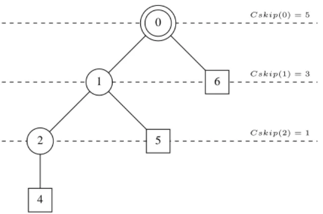
Each router is allocated an address space. The first address of the address space is used as the address of the router itself, and the remaining addresses are distributed to its children. The length of the address space given to a router at depth d+ 1, called Cskip(d), is computed as follows (see paragraph 3.6.1.6 of [5]): Cskip(d) = ( 1 + Cm· (Lm− d − 1) if Rm= 1, 1+Cm−Rm−Cm·RLm−d−1m 1−Rm otherwise.
The PAN coordinator address is always 0. A parent device that has a Cskip(d) greater than zero can accept devices as children and can assign addresses. If Cskip(d) is zero, it can not have children devices and then it must be treated as an end-device. If a parent node of depth d is assigned an address Aparent, the address Ak of its k-th router and the address An
of its n-th end-device are calculated according to the following equations: Ak= Aparent+ Cskip(d).(k − 1) + 1, An= Aparent+ Cskip(d).Rm+ n. 2 1 5 6 4 0 Cskip(0) = 5 Cskip(1) = 3 Cskip(2) = 1
Figure 1. Example of the distributed address allocation scheme with Cm= 2, Rm= 1and Lm= 3.
Figure 1 shows an example of the distributed address allocation scheme, where the PAN coordinator is represented by a double circle, the routers are represented by circles and the end-devices are represented by squares. The network parameters are assigned the following values: Cm = 2,
Rm= 1 and Lm= 3. The PAN coordinator has 0 as address.
In this example, we have Cskip(0) = 1 + Cm·(Lm− d− 1) =
1 + 2 · 2 = 5. Thus, the router child of the PAN coordinator is assigned the address1 and the end-device child is assigned the address1 + Cskip(0) = 6.
2) Hierarchical tree routing protocol: The hierarchical tree routing protocol (see paragraph 3.6.1.6 of [5]) is based on the distributed address allocation scheme. End-devices forward messages to their parent routers. When a router receives a message for a destination, it checks whether the destination is within its own address space or not. If it is the case, the destination is a descendent of the router. The router determines which child router the destination belongs to, and sends the message to the concerned child. If it is not the case, that is if the destination is not within the address space of the router, the router sends the message to its parent.
Let us consider the topology shown on Fig. 1, and let us suppose that a message is sent from the end-device 6 to the end-device 4. End-device 6 sends the message to its parent, which has address 0. Router 0 (which is the PAN coordinator) has to determine if the destination 4 is within its address space [0; 6] or not. As it is the case, the destination 4 is a descendant of the router 0. Then, the router has to determine if the destination is one of its children, or if the message has to be sent to an intermediate child router. In this case, the router 0 detects that the destination 4 is within the address space of its child 1, so it forwards the message to the router 1. Router 1 has to determine if the destination 4 is within its address space[1; 5] or not. As it is the case, the destination 4 is a descendant of the router 1. The same process is repeated and router 1 sends the message to its child 2. Then, router 2 detects that the destination 4 is within its address space[2; 4] and that it is its own child. Thus, it sends the message to the destination 4.
advantage of the MAC layer associations to perform the routing functionality. This protocol is a simple proactive routing protocol based on the distributed address allocation scheme described in the previous paragraph. Routes towards a destination are established before any sensor node needs to perform packet routing. The main advantages of this routing protocol are its simplicity and its limited use of resources. Indeed, it does not require additional control messages or complex routing tables.
The main drawback of protocols based on the hierarchical tree routing is the fact that the routing paths are not optimized. Indeed, the messages always follow the tree topology, even if shortest paths exist.
3) Neighbor routing protocol: The neighbor routing pro-tocol (see paragraph 3.6.3.3 of [5]) improves the hierarchical tree routing by using one-hop neighbor tables. When a router has to forward a message to a destination, it first checks if the destination is physically within communication range, i.e., if the destination is in its neighbor table. If it is the case, the router sends the message directly to the destination. Otherwise, it follows the hierarchical tree routing protocol.
C. AODV routing protocol
AODV [1] is a reactive routing protocol: routes to desti-nations are acquired in an on-demand manner. When a node has to route packets to a destination, it broadcasts a Route REQuest (RREQ) message. As this message is spread through the network, each node that receives it sets up a reverse route, i.e., a route towards the requesting node. As soon as a RREQ message reaches a node with an established route to the destination (including the destination itself), a Route REPly (RREP) unicast message is sent back to the requesting node. Intermediate nodes use the reverse routes to forward RREP messages.
However, reactive routing protocols, such as AODV, con-tribute to a significant end-to-end delay due to the time required to establish the route.
D. Shortcut tree routing protocol
The shortcut tree routing protocol [7] improves the hier-archical tree routing by using one-hop neighbor tables and shortest paths. When a router has to forward a message to a destination, it computes the expected distance from each neighbor (including its parent and its children) to the destina-tion according to the hierarchical tree routing. Then, it sends the message to the nearest neighbor to the destination.
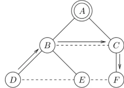
Figure 2 illustrates an example of the shortcut routing protocol. Router D has to send a message to router F . For each neighbor, D computes the expected distance to the destination F . For neighbor B, the expected path is (B, A, C, F ) and the distance is 3. For neighbor E, the expected path is (E, B, A, C, F ) and the distance is 4. Therefore, router D sends the message to its neighbor B. For each neighbor, router B computes the expected distance to the destination F . For neighbor D, the expected path is (D, B, A, C, F ) and the distance is 4. For neighbor A, the expected path is(A, C, F )
A
B C
D E F
Figure 2. An example of the shortcut tree routing protocol.
and the distance is 2. For neighbor E, the expected path is (E, B, A, C, F ) and the distance is 4. For neighbor C, the expected path is (C, F ) and the distance is 1. Therefore, the router B sends the message to its neighbor C. Router C detects that the destination F is one of its neighbors, and sends the message directly to it.
III. PIRATPROTOCOL
In this section, we show that reactive routing protocols and proactive deterministic routing protocols produce congested areas in the network. Then, we propose the PiRAT (Pivot Routing for Alarm Transmission) protocol in order to deal with this problem. Finally, we describe the topology and our modeling of the alarm traffic.
A. Problem of congestion due to alarms
Congestion is defined as the state when a node receives more packets than it can transmit. As nodes use a shared radio medium, congestion occurs in areas where congested nodes are located [8].
Congestion happens when a limited area of the network generates most of the data towards the same destination. Moreover, congestion increases as the data generation rate of the alarm traffic increases. The radio range also affects the congestion of nodes: when the radio range increases, the number of nodes in range of each other increases, and the access to the medium becomes more difficult.
Congestion negatively impacts the performance of the net-work. First, as the congestion increases, the contention for the medium also increases, which results into more collisions. Collisions result into packet losses and retransmissions. Re-transmissions require energy and lead to an increase in the end-to-end delay. Second, the congested nodes have to buffer the packets in their queues, which increases the delay.
Reactive protocols, such as AODV, are not suitable for alarm traffic transmission due to the time needed to establish the routes. Moreover, such protocols cause high overhead in order to establish the routes [9][6]. For example, in AODV, the routers broadcast RREQ messages in the whole network, for each source-destination pair.
Deterministic proactive protocols, such as the hierarchical tree routing and the shortcut protocols, produce important congestion. Indeed, those protocols are deterministic, which means that the packets always follow the same routes. As
packets approach the destination, the routes converge and the amount of traffic to be routed dramatically increases, which overloads all the nodes near the destination, and leads to a bottleneck.
B. PiRAT protocol description
The PiRAT protocol provides a simple solution that aims to reduce the congestion induced by alarm transmission in a wire-less sensor network. It uses two steps. The first step consists in selecting pivot nodes for each source-destination pair (see Subsect. III-C). The second step consists in forwarding alarm packets via a randomly chosen pivot node to the destination. Thus, PiRAT is a probabilistic proactive protocol.
The PiRAT protocol is based on diversity routing due to its probabilistic nature, and also on the shortcut routing protocol. Indeed, the paths from the source to the pivot and from the pivot to the destination are computed according to the shortcut tree routing. PiRAT possesses another probabilistic feature. When several neighbors lead to a destination with the same minimum distance, PiRAT chooses one of these nodes randomly.
The main advantage of PiRAT is that it provides multi-path routing to the destination. Indeed, it allows a larger number of nodes to participate in the routing activity. Thus, the energy usage is more balanced among the nodes of the network than with deterministic proactive protocols. This feature has the benefit of extending the lifetime of the network.
C. Selection of the pivot nodes
Selecting pivots is the key aspect of the PiRAT protocol. Selecting pivots close to the shortest path from the source to the destination reduces the hop count but also increases the congestion. Selecting pivots far from the shortest path from the source to the destination increases the hop count and the delay. The distance between pivot nodes is also an important issue in order to avoid interferences between paths.
We propose to select the pivots in a large area in order to avoid the convergence of paths and thus balance the load of alarm traffic in the network. A sensor node is considered as a pivot if it satisfies the following conditions:
1) its distance from the source is strictly greater than its distance to the sink,
2) it is not located on the shortest path from the source to the destination,
3) it is not located on the boundaries of the network. The first condition ensures that the pivot is closer to the destination than to the source. This is required to push the path convergence as far away as possible from the source. The second condition ensures that the path via the pivot does not follow the shortest path from the source to the destination, which is the most congested area. The third condition is needed as nodes on the boundaries of the network have less routing options than the other nodes, which reduces the available routing diversity and increases congestion on the boundaries.
The distance used in the previous conditions is ideally the physical distance between nodes. However, as nodes have no knowledge of their geographical positions, we propose to consider the number of hops according to the shortcut tree routing as our distance. This metric is better than the number of hops computed according to the hierarchical tree routing, as it is based on the environment (through the neighbor tables) rather than on the tree topology only.
Once a source has determined a set of possible pivot nodes, it randomly chooses one of them. Then, packets are routed through this pivot.
The pivot selection protocol is the following. First, we assume that the nodes that are located in the potential alarm areas know by advance that they are potential sources. Thus, they initiate a pivot discovering phase by broadcasting a Pivot Discovery Message (PDM). This message contains the distance between the source s and the destination d (computed according to the shortcut tree routing). When a node n receives a PDM, it verifies that all the three following conditions hold:
• d(s, n) > d(n, d),
• d(s, n) + d(n, d) > d(s, d) + ε1, where ε1 is a threshold
chosen according to the network size,
• the number of neighbors of n is greater than a threshold
ε2.
All the nodes that satisfy the three conditions are candidates for the pivot selection. Each candidate sends a Pivot Notifi-cation Message (PNM) to the source to inform it that it is a potential pivot. Once the source has received a given number of PNM, or has waited for a given time duration, it chooses randomly one of them to be its dedicated pivot.
D. Topology description and alarm traffic production
In the following simulations, we considered for simplicity reasons a set of 100 sensor nodes uniformly distributed on a 100 m×100 m grid. All sensors are FFD and operate on the non-beacon-enabled mode. The PAN coordinator is located at the center of the area. The network parameters are defined as follows: Cm = 5, Rm = 5 and Lm = 5. We varied
the radio range from 30 m to 40 m. Figure 3 shows an example of the associations between nodes using the parent-child relationships with a fixed association range of 20 m. We define the association range as the maximum distance between a parent and a child. It is smaller than the radio range in order to ensure that nodes are associated through high quality links. As it can be seen on the figure, nodes are randomly associated with each other. For example, if the sensor node 20 has to transmit a packet to the sensor 50 according to the hierarchical tree routing protocol, the following path is used: (20, 22, 23, 34, 45, 54, 52, 50).
The alarm traffic is produced in the following way. First, we assume that an emergency event occurs at the bottom left-hand corner of the network. This event is detected by all the sensors located within a given radius. In our simulations, we set the detection radius to 25 m. Thus, eight nodes are sources. Notice that the event occurs in the network after all the associations are performed and the pivot selection algorithm is
0 1 2 3 4 5 6 7 8 9 10 11 12 13 14 15 16 17 18 19 20 21 22 23 24 25 26 27 28 29 30 31 32 33 34 35 36 37 38 39 40 41 42 43 44 45 46 47 48 49 50 51 52 53 54 55 56 57 58 59 60 61 62 63 64 65 66 67 68 69 70 71 72 73 74 75 76 77 78 79 80 81 82 83 84 85 86 87 88 89 90 91 92 93 94 95 96 97 98 99
Figure 3. Example of node associations: lines represent parent-child relationships.
accomplished. There is no background traffic as we focus on the alarm traffic only. We assume that the sink is located in the top right-hand corner. All the nodes of the network participate to the multi-hop routing process. Finally, we assume that the alarm notifications last for 30 seconds and we vary the alarm data rate from 1 packet per second to 30 packets per second. Alarm notifications are produced periodically to inform the sink of the evolution of the event in a real-time manner.
E. Performance metrics
PiRAT is evaluated and compared to the existing protocols according to several performance metrics:
• End-to-end delay: the end-to-end delay is the time
inter-val between the transmission of a packet by the source and the reception of the same packet by the sink. Thus, the end-to-end delay only takes into account the packets that are correctly received.
• Packet loss: the packet loss is defined as the ratio of the
number of packets successfully received by the sink over the number of packets generated by the source nodes. Thus, the packet loss ratio takes into account the losses due to collisions or queue overflows.
• Number of hops: the number of hops is defined as
the number of intermediate nodes required to forward a packet from the source to the sink. Only the packets received by the sink are considered.
• Node usage: the node usage indicates how many sensor
nodes are used in the routing process, and how many times they have to forward packets.
IV. SIMULATION RESULTS
In this section, we describe the extensive simulations that we conducted in order to evaluate PiRAT. Simulations are carried
out using the network simulator NS2 [10], version 2.31. We used the existing implementation of the IEEE 802.15.4 PHY and MAC layers. We used the two ray ground propagation model (with default parameters). The transmission power is set to a realistic value of 3.16 µW, which is -25 dBm, and the reception threshold is set to 0.347412 pW (for a radio range of 30 m) or 0.195419 pW (for a radio range of 40 m). NS2 also requires the user to specify a carrier sense threshold. The carrier sense threshold is equal to the reception threshold as the IEEE 802.15.4 throughput is limited to only 250 kbps. We decided to limit the size of the nodes queue to 5 packets of 34 bytes (at the PHY layer), due to their limited storage capabilities.
We compared the PiRAT protocol with the hierarchical tree routing protocol, referred to as tree, and the shortcut tree routing protocol, referred to as shortcut. We studied AODV as an example of the reactive routing protocols.
Each simulation is performed over one hundred repetitions. We displayed the 95% confidence interval on the following figures.
A. Route establishment time with AODV
We used the existing implementation of AODV in NS2. In order to show the inefficiency of AODV for alarm transmissions in wireless sensor networks, we considered a simple topology of 100 nodes, uniformly distributed in a 100 m×100 m area. We selected the node 0 as source and the node 45 (the center of the network) as the destination, and we measured the delay for each packet when the source transmits one packet per second. AODV tries to establish several routes from the source to the destination, in case the optimal route becomes congested. This takes a significant time.
Figure 4 plots the average end-to-end delay for each packet correctly received. We can see on the figure that the packets suffer from a large delay. This is due to the fact that the source broadcasts RREQ messages to its neighbors in order to establish an optimal route to the destination. Thus, the route discovery penalizes the transmission delay of the first generated packets. 0 1 2 3 4 5 6 7 8 9 10 20 25 30 35 40 45 50
End−to−end delay (seconds)
Packet ID
Figure 4. Average end-to-end packet delay with AODV: on this example, it takes 9 seconds to establish the route.
As we can see in Fig. 4, the transmission delay of the first received packet is about 9 seconds and about 8 seconds for the
second packet. For each packet, the average delay decreases by one second because packets are transmitted with a rate of one packet per second. After the ninth packet (ID 29), the time of route establishment has no effect on the end-to-end delay. However, we observe a significant delay for the packets having the IDs 30 and 31. These delays are due to the reestablishment of the route between the source node and the sink. Note that the packets having an ID from 1 to 19 have been dropped because AODV was unable to establish a route.
These simulation results show that AODV is not suitable as an alarm routing protocol because of the large end-to-end delay it causes. Because of this drawback, we concentrate the remaining of our study on the proactive routing protocols only.
B. End-to-end delay
Figure 5 and Fig. 6 show the mean end-to-end delay between the generation and the reception of a packet, as a function of the frequency of the alarm transmission rate with a radio range of 30 m and 40 m respectively.
For the hierarchical tree routing, the delay increases quickly and becomes stable after 15 packets per second. This is due to the fact that routes are long and the number of retransmissions is high (as the packet loss is high, see Subsect. IV-C). As the data transmission rate increases, the packet loss becomes higher and several packets are dropped. The packets most likely to be dropped are those that correspond to long routes. Only packets that follow short routes are received by the destination, which reduces the end-to-end delay.
For the shortcut tree routing and PiRAT, the delay in-creases with the data transmission rate. This is mainly due to the increasing congestion and the necessary retransmissions. However, these two protocols outperform the hierarchical tree routing. When the alarm transmission rate is high, PiRAT has the best behavior in terms of delay. The end-to-end delay reduction of PiRAT over shortcut reaches 28% when the alarm transmission rate reaches 30 packets per second, for a radio range of 30 m, and 40% for a radio range of 40 m. When the radio range increases, shortcut and PiRAT have better performances as nodes have more neighbors to route packets to. 0 0.02 0.04 0.06 0.08 0.1 0.12 0.14 0 5 10 15 20 25 30
End−to−end delay (seconds)
Data transmission rate (packets per second) Tree
Shortcut PiRAT
Figure 5. Average end-to-end delay for a radio range of 30 m.
0 0.02 0.04 0.06 0.08 0.1 0.12 0.14 0 5 10 15 20 25 30
End−to−end delay (seconds)
Data transmission rate (packets per second) Tree
Shortcut PiRAT
Figure 6. Average end-to-end delay for a radio range of 40 m.
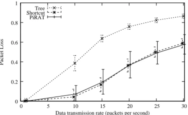
C. Packet loss
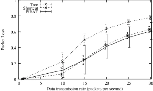
Figure 7 and Fig. 8 show the mean packet loss as a function of the frequency of the alarm transmission rate with a radio range of 30 m and 40 m respectively. We notice that the packet loss for all the protocols increases consistently with the data transmission rate. As the hierarchical routing protocol uses long paths, the probability of loosing packets is high. It can reach up to 80% for 30 packets per second and a radio range of 30 m, and up to 85% for 30 packets per second and a radio range of 40 m. The shortcut and PiRAT protocols are able to achieve lower packet loss rates by shortening the paths from the sources to the destination. They achieve only 60% of packet loss rates for 30 packets per second and both radio range. 0 0.2 0.4 0.6 0.8 1 0 5 10 15 20 25 30 Packet Loss
Data transmission rate (packets per second) Tree
Shortcut PiRAT
Figure 7. Average packet loss for a radio range of 30 m.
D. Number of hops
Figure 9 and Fig. 10 represent the average number of hops as a function of the alarm transmission rate. As expected, the number of hops does not depend on the network load. With the hierarchical tree routing, packets suffer from paths of 9 hops independently from the radio range. Only the association range is taken into account in the hierarchical tree routing protocol. In our simulations, we set this range to 20 m. The shortcut routing algorithm decreases the number of hops since it routes packets via a short path. We notice an average path length of 5.5 hops for a radio range of 30 m and an average path length of 4.4 hops for a radio range of 40 m. This is due to the fact
0 0.2 0.4 0.6 0.8 1 0 5 10 15 20 25 30 Packet Loss
Data transmission rate (packets per second) Tree
Shortcut PiRAT
Figure 8. Average packet loss for a radio range of 40 m.
that as the radio range increases, more neighbors can be used to shortcut the tree. With PiRAT, the routes are longer than those used by the shortcut tree routing, but our pivot selection algorithm ensured that the number of hops does not become too large. The average path length for PiRAT consists of 6.5 hops for a radio range of 30 m and of 4.8 hops for a radio range of 40 m. 4 5 6 7 8 9 10 11 0 5 10 15 20 25 30 Hop number
Data transmission rate (packets per second) Tree
Shortcut PiRAT
Figure 9. Average number of hops for a radio range of 30 m.
3 4 5 6 7 8 9 10 11 0 5 10 15 20 25 30 Hop number
Data transmission rate (packets per second) Tree
Shortcut PiRAT
Figure 10. Average number of hops for a radio range of 40 m.
E. Node usage
The node usage metric is the most important metric for PiRAT. PiRAT improves the shortcut routing algorithm by using diversity in routing and decreasing the congested areas in
the network. With PiRAT, only the area around the destination is congested (see Fig. 11 and Fig. 12).
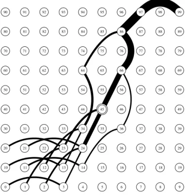
Figure 11 shows the participation of all the nodes in the routing process for the shortcut tree routing protocol. Sources are nodes 0, 1, 2, 10, 11, 12, 20 and 21. A thick line indicates that the link is used multiple times while a thin line indicates that a link is rarely used. As we can see, the routes used by the shortcut tree routing protocol share a significant number of nodes. The large number of thick lines proves that the shortcut tree routing protocol causes congestion along the common path. Moreover, as soon as one of the nodes of the path drains its energy because it has transmitted too many packets, the route becomes inactive and the network lifetime decreases.
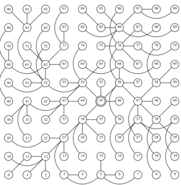
Figure 12 shows the participation of all the nodes in the routing process for the PiRAT protocol. The pivot nodes selected by the sources are represented using dashed circles. The routes from the sources to the destination avoid the central area in order to reduce congestion. The probabilistic nature of PiRAT can be seen as each node uses several paths to reach a given destination (either the pivot node or the sink). While the shortcut tree routing protocol used 21 nodes, PiRAT uses a total of 42 nodes. Thus, PiRAT doubles the number of nodes used, and then, it reduces the amount of the transmitted packets per node. This leads to reduce the overloaded paths and balance the energy consumption of the nodes. This phenomenon greatly improves the network lifetime.
As we can see on Fig. 11, the path from the PAN (node 45) to the sink (node 99) via the intermediate nodes 66, 86, and 97 is overloaded. This is due to the fact that all the packets follow the same path. However, as it can be seen on Fig. 12, the nodes used by the shortcut protocol are less solicited to route packets when the PiRAT protocol is used. With PiRAT, new nodes participate in the routing process; the traffic load is reduced for each node. Indeed, because of the diversity in routing, node 45 sends packets to nodes 47 and 75 and does not use the wireless link (45-66). Then, node 86 receives less packets from more nodes (56, 68, 83, 84) than on Fig. 11. The same phenomenon occurs at node 97, which reduces the congested areas. However, since the destination is always the same (node 99), the sink is always overloaded with both protocols. Thus, the area around it is congested.
V. CONCLUSION
In this paper, we showed that congestion is a major issue when dealing with alarms in a wireless sensor network. We proposed a new protocol called PiRAT which uses pivot nodes in order to add diversity to the routing process. It also adds diversity to the shortest paths it uses in routing packets. Simulation results showed that PiRAT outperforms the reactive protocols as well as the proactive deterministic routing tree protocols in terms of end-to-end delay (reduction up to 60% and 28% for a communication range of 30 m, and up to 80% and 40% for a communication range of 40 m compared to the hierarchical tree routing protocol and the shortcut tree routing protocol respectively), without negatively impacting
0 1 2 3 4 5 6 7 8 9 10 11 12 13 14 15 16 17 18 19 20 21 22 23 24 25 26 27 28 29 30 31 32 33 34 35 36 37 38 39 40 41 42 43 44 45 46 47 48 49 50 51 52 53 54 55 56 57 58 59 60 61 62 63 64 65 66 67 68 69 70 71 72 73 74 75 76 77 78 79 80 81 82 83 84 85 86 87 88 89 90 91 92 93 94 95 96 97 98 99
Figure 11. Node usage with the shortcut tree routing protocol.
000 000 000 000 111 111 111 111 000 000 000 000 111 111 111 111 000 000 000 000 111 111 111 111 000 000 000 000 111 111 111 111 000 000 000 000 111 111 111 111 000 000 000 000 111 111 111 111 0 1 2 3 4 5 6 7 8 9 10 11 12 13 14 15 16 17 18 19 20 21 22 23 24 25 26 27 28 29 30 31 32 33 34 35 36 37 38 39 40 41 42 43 44 45 46 47 48 49 50 51 52 53 54 55 56 57 58 59 60 61 62 63 64 65 66 67 68 69 70 71 72 73 74 75 76 77 78 79 80 81 82 83 84 85 86 87 88 89 90 91 92 93 94 95 96 97 98 99
Figure 12. Node usage with the PiRAT protocol.
the packet loss. Moreover, PiRAT performs better than the existing routing protocols in terms of congestion as it uses a larger number of nodes while routing packets from source to destination. This leads to a good balancing of the energy usage, which in turn extends the network lifetime.
The perspectives of this work include the optimization of the pivot selection algorithm, the reduction of the number of messages required to select the pivot candidates, and the packet loss reduction.
VI. ACKNOWLEDGMENT
This work has been partially supported by a research grant from the Lebanese National Council for Scientific Research (LNCSR).
REFERENCES
[1] C. Perkins, E. Belding-Royer, and S. Das, “Ad hoc on-demand distance vector (AODV) routing,” IETF, Request For Comments 3561, July 2003. [2] IEEE 802.15, “Part 15.4: Wireless medium access control (MAC) and physical layer (PHY) specifications for low-rate wireless personal area networks (LR-WPANs),” ANSI/IEEE, Standard 802.15.4 R2003, 2003. [3] J. Zheng and M. J. Lee, “Will IEEE 802.15.4 make ubiquitous network a reality?: A discussion on a potential low power, low bit rate standard,”
IEEE Communications Magazine, vol. 27, no. 6, pp. 23–29, 2004. [4] E. Callaway, P. Gorday, L. Hester, J. Gutierrez, M. Naeve, B. Heile, and
V. Bahl, “Home networking with IEEE 802.15.4: A developing standard for low-rate wireless personal area network,” IEEE Communications
Magazine, vol. 40, no. 8, pp. 70–77, 2002.
[5] ZigBee, “ZigBee Specification,” ZigBee Standards Organization, Stan-dard Zigbee 053474r17, January 2008.
[6] F. Cuomo, S. Della Luna, U. Monaco, and F. Melodia, “Routing in ZigBee: Benefits from exploiting the IEEE 802.15.4 association tree,” in IEEE International Conference on Communications (ICC), 2007, pp. 3271–3276.
[7] T. Kim, D. Kim, N. Park, S.-E. Yoo, and T. S. L ´opez, “Shortcut tree routing in ZigBee networks,” in ISWPC, 2007.
[8] A. P. Jardosh, K. M. Ramachandran, K. C. Almeroth, and E. M. Belding-Royer, “Understanding congestion in IEEE 802.11b wireless networks,” in Internet Measurement Conference, 2005.
[9] R. Kumar, R. Crepaldi, H. Rowaihy, A. F. Harris, G. Cao, M. Zorzi, and T. F. La Porta, “Mitigating performance degradation in congested sensor networks,” IEEE Transactions on mobile computing, vol. 7, no. 6, pp. 682–697, 2008.