Bifurcation analysis and control of a fighter aircraft

Bifurcation Analysis

arid Control of a Fighter

Aircraft

by

Pierre-Etienne AUBIN

Ancien Aleve de l'Ecole polytechnique, Palaiseau, France (1987-1990)

Ingenieur de l'armement

Submitted to the Department of Aeronautics and Astronautics

in partial fulfillment of the requirements for the degree of

Master of Science in Aeronautics and Astronautics

at the

MASSACHUSETTS INSTITUTE OF TECHNOLOGY

February 1993

@

Pierre-Etienne AUBIN, MCMXCIII. All rights reserved.

The author hereby grants to MIT permission to reproduce and to

distribute copies

of this thesis document in whole or in part, and to grant others the

right to do so.

'- J

Author ...

Certified by...

Department of Aeronautics and Astronautics

December 8, 1992

i . ,. V ...

Rudrapatna V. Ramnath

Adjunct Professor of Aeronautics and Astronautics

Thesi Supervisor

Accepted by ...

FEB 17 1993

Professor Harold Y. Wachman

Chairman, Departement Graduate Committee

Bifurcation Analysis and Control of a Fighter Aircraft

by

Pierre-Etienne AUBIN

Submitted to the Department of Aeronautics and Astronautics on December 8, 1992, in partial fulfillment of the

requirements for the degree of

Master of Science in Aeronautics and Astronautics

Abstract

The equations of flight dynamics can be written in the form of a first order system of nonlinear differential equations. Linear approximations of this system are usually accurate enough to deal with low amplitude maneuvers involving only small angles of attack and sideslip. However, to predict the behavior of a plane at high angle of attack, one has to cope with many nonlinearities, both in the aerodynamic coefficients and in the mathematical model itself.

In this thesis, a system including nonlinear aerodynamic coefficients have been studied from the standpoint of the bifurcation theory. The bifurcation theory basically allows us to analyze how the equilibrium states of a differential system vary when parameters (typically, deflections of the rudder, the elevator or the ailerons) are varied. This bifurcation analysis was successfully employed to predict such nonlinear phe-nomena as sudden jumps or departures into limit cycles. The occurrence of these phenomena have been confirmed by numerical simulations and time histories. Some applications of the bifurcation theory to control problems were investigated. Specifi-cally, a control system aimed at avoiding jumps during lateral maneuvers was designed and the bifurcation surface concept was applied to the design of a classical control system, namely a yaw damper.

Thesis Supervisor: Rudrapatna V. Ramnath Title: Professor of Aeronautics and Astronautics

Acknowledgements

I want to thank the Del6gation Generale pour l'Armement of the French Ministry of Defense for supporting my studies at MIT.

I want to express my gratitude to Professor Rudrapatna V. Ramnath for giving me the opportunity to work on these original mathematical approaches to flight dynamics, for his guidance and friendliness and for his patient correction of this thesis.

I would like to thank all the people who have helped me and made my life easier, especially Mrs. Edith Roques at Sup'Aero, who helped so much in preparing my application to MIT, Mrs. Valentine Girard at the French Embassy, Mrs. Elizabeth Zotos in the Aero/Astro Department at MIT, Pierre-Henri at the French Consulate, the Medical Department, the libraries and the Athena network staff.

Among all the friends we met this year, I am especially grateful to the Mahoney family. More than friends, you are now our American family.

Thank you also to Art and Margaret Kalb, Nancy Daly, Lynn Page, Karina and Eng-Soon Chan, Yuko and Takashi Maekawa, Christian Malis and Loic Batel. You all deserve a gold medal in baby-sitting.

A very special thanks also to Etienne and Gwenaalle Balmbs. Your support and friendship helped us a lot. We hope you will come and join us in Paris next year.

To all our relatives who have crossed the Atlantic to help and visit us, merci! Laure, Priscille, Laetitia and Henri, our American boy, this work is certainly not a masterpiece but it is for you, with all my love as a husband and a dad.

Contents

1 Introduction

1.1 Linear and nonlinear models in flight dynamics . . . .

1.1.1 Linear m odels . ... .. ... .. ..

1.1.2 "Maneuverability [...], the difference between life and death"

1.1.3 Aerodynamic peculiarities of flight at high angle of attack . . 1.1.4 The bifurcation theory, a new powerful tool in nonlinear flight

dynam ics . . . . 1.2 Statement of purpose ...

1.3 Organization of the report ... 2 Introduction to the Bifurcation Theory

2.1 Introduction .... .... ... 2.2 The linear system ~ = Ax ...

2.2.1 General theory ...

2.2.2 The two dimensional case . . . .

2.3 Invariant spaces ...

2.4 The nonlinear system - = f(x) . . . .

2.4.1 The non degenerate equilibrium case . . . . 2.4.2 The degenerate equilibrium case . . . .

2.5 Center manifolds and the center manifold theorem . 2.6 Stability of center manifolds . . . . 2.7 Bifurcation theory ... 2.7.1 Introduction ... 20 ... . 20 S. . . 21 . . . . 21 S. . . 22 S. . . 25 S. . . 26 S . . . 27 * . . . 29 S. . . 29 S . . . 31 .. . . 33 S. . . 33

2.7.2 2.7.3

2.7.4

Basic bifurcation models ... .. 33

Saddle-node, transcritical and pitchfork bifurcations ... 37

Hopf bifurcation ... 39

3 Bifurcation Analysis of the Longitudinal and Lateral Dynamics of a fighter Aircraft 40 3.1 3.2 Introduction ... Introductory example: an airplane model in a 3.2.1 Description and equations of motion 3.2.2 Equilibrium points ... 3.3 Longitudinal dynamics of a fighter . . . . . 3.3.1 General equations ... 3.3.2 Equilibrium points ... 3.3.3 Results and interpretation... 3.4 Lateral dynamics of a fighter ... 3.4.1 General equations ... 3.4.2 Equilibrium points ... 3.4.3 Interpretation ... 4 Control strategies 4.1 Introduction ... 4.2 Longitudinal control ... 4.2.1 Control system design ... 4.2.2 Examples ... 4.3 Lateral control ... 4.3.1 Bifurcation surfaces ... 4.3.2 Use of bifurcation surfaces to design 4.4 Another application of bifurcation surfaces . . . . 40 wind tunnel . ... 41 S . . . . . 41 . . . . 43 S . . . . . 45 . . . . 45 . . . . 48 . . . . 50 . . . . 58 . . . . 58 . . . . 59 . . . . 60 74 . . . . 74 . . . . 75 . . . . 75 . . . . 75

the lateral control system

5 Summary and conclusions

5.1 Introduction .. . . .. . . ... .... .. .. ... .. .. .. .. ..

87

5.2 The bifurcation theory ... 88

5.3 Bifurcation analysis of the longitudinal and lateral dynamics of a fighter aircraft . . . .. .. . 90

5.3.1 Longitudinal dynamics ... 90

5.3.2 Lateral dynamics ... 91

5.4 Control strategies ... ... 93

5.5 Conclusions and recommendations for further work . ... 95

5.5.1 Conclusions ... 95

5.5.2 Recommendations for further work . ... 95 A Matlab routine used to compute the value and the stability of the

equilibrium states of the system 2.16 97

List of Figures

1-1 Aerodynamic hysteresis on the rolling moment coefficient ... 17

2-1 Stable node (left) and unstable node . ... 22

2-2 Saddle . . . .. .. . . . . .. . . . .. . 23

2-3 Proper node (left) and improper node . ... . . . . . 24

2-4 Vortex .. . .. .. .. . . ... .. .. .. .. ... .. .. .. . .. . 24

2-5 Stable focus (left) and unstable focus . ... 25

2-6 Invariant subspaces for matrix A . ... . 27

2-7 Nonlinear and linearized flow near an hyperbolic equilibrium point (left). Stable and unstable manifolds and subspaces . ... 29

2-8 Stable, unstable and center manifolds and subspaces ... 30

2-9 Local phase portrait and center manifold for system 2.12 and a > 0 . 33 2-10 Bifurcation diagram for the saddle-node bifurcation . ... 34

2-11 Bifurcation diagram for the transcritical bifurcation . ... 34

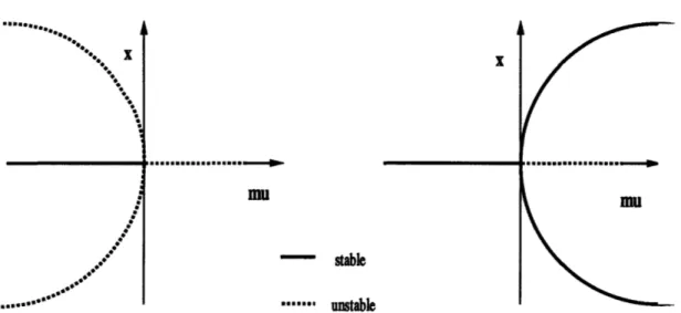
2-12 Bifurcation diagrams for the subcritical (left) and supercritical pitch-fork bifurcation ... 35

2-13 Bifurcation diagram for the Hopf bifurcation . ... . . . 35

2-14 Two-dimensional center manifold for system 2.17 . ... . . 37

3-1 Geometry and notations for the airplane model . ... 41

3-2 Linear and nonlinear aerodynamic moments . ... 42

3-3 Bifurcation diagram for the airplane model. Equilibria marked with 'O' are unstable ... ... 44

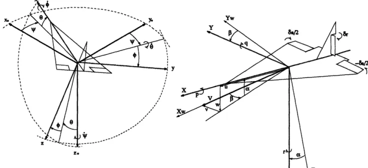
3-4 _{Orientations of earth (Xe, Ye, Ze), body (X, Y, Z) and wind (Xw, Yw,} Zw) axes, linear and angular velocities and control deflections (the elevator deflection does not appear on this Figure: 6e is positive when

the trailing edge of the elevator is down) . ... 46

3-5 Equilibrium diagram for flight conditions I. Equilibria marked with 'o' are unstable .. . . . . 51 3-6 Equilibrium diagram for flight conditions II. Equilibria marked with

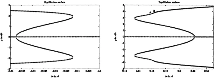
'o' are unstable . . . . 51 3-7 Enlargements of the equilibrium surface for negative Se (left) and

pos-itive Se . . . . 52 3-8 Eigenvalues of the stabilty matrix for 0.13 rad < Se < 0.25 rad,

corre-sponding to the trivial solution p = 0 (left) and to the stable branch

of the saddle-node bifurcation (right) . ... 53

3-9 Eigenvalues of the stabilty matrix for -0.34 rad < 6e < -0.30 rad,

corresponding to the trivial solution p = 0 . ... 54

3-10 Simulation just before the Hopf bifurcation on simplified system 3.16

(left) and original system 3.15 ... 55

3-11 Simulation just beyond the Hopf bifurcation on simplified system 3.16

(left) and original system 3.15 ... 56

3-12 Shape of the limit cycle for Se = 0.25 for simplified system 3.16 (left)

and original system 3.15 ... 56

3-13 Attraction towards the limit cycle for 6e = 0.20. pi~i = 2.5 rad/s in the case of system 3.16 and pini = 4 rad/s in the case of system 3.15 . 57 3-14 Attraction towards the trivial solution for Se = 0.20. pai, = 0.5 rad/s

in both cases . . . .. . 57 3-15 Left: jump to high values of the state vector. The simplified system

3.16 is used for the simulation ... 58

3-16 Right: jump to high values of the state vector. The complex system

3.15 is used for the simulation ... 58

3-18 Equilibrium diagrams for be = -0.2 rad. The 'o' points are unstable.. 62

3-19 Equilibrium diagrams for be = 0 rad. The 'o' points are unstable. .. 63

3-20 Equilibrium diagrams for be = 0.10 rad. The 'o' points are unstable.. 64

3-21 Equilibrium diagrams for Se = 0.15 rad. The 'o' points are unstable.. 65

3-22 Equilibrium diagrams for be = 0.30 rad. The 'o' points are unstable.. 66

3-23 Simulation of a jump for be = 0 rad and Sr = -0.3 rad. Simulation on the simplified system is on the left. ... 67

3-24 Equilibrium diagram for Se = -0.20 rad, Sr = -0.20 rad ... 68

3-25 Eigenvalues diagram for be = -0.20 rad and Sr = -0.20 rad ... 68

3-26 Subcritical Hopf bifurcation ... 69

3-27 Simulation for Se = 0.15 rad and Sr = 0 rad, when da goes from 0 to 0.066 rad ... . ... ... .. 70

3-28 Equilibrium diagram for be = 0.30 rad and Sr = -0.30 rad ... 72

3-29 Simulation of a limit cycles for Se = 0.30 rad and Sr = -0.3 rad. Sim-ulation on the simplified system is on the left. . ... 72

3-30 Bifurcation diagram for two successive Hopf bifurcations ... . 72

3-31 Eigenvalues diagram for be = 0.30 rad and Sr = -0.30 rad ... . 73

4-1 Time histories showing the instability of the airplane when either a large positive (right) or negative (left) elevator deflection step is applied 76 4-2 Time histories when a control system stabilizes the airplane after a per-turbation. Cases of a large negative (left) and positive (right) elevator deflection step. ... 77

4-3 Time histories of the aileron deflection when a control system stabilizes the airplane after a perturbation. Cases of a large negative (left) and positive (right) elevator deflection step. . ... 77

4-4 Bifurcation surface in the control space (Sr, Sa), for Se = -0.20 rad. The figures inside the diagram indicate the number of equilibrium states in each area . . . . 78

4-6 Simulation of a jump for Se = -0.20 rad and Sr = 0 rad, when 6a varies

linearly from 0 to 1 rad ... 79

4-7 Bifurcation surface and definition of the ailerons-rudder coupling in the control space (Sr, Sa), for Se = -0.20 rad. The figures inside the

diagram indicate the number of equilibrium states in each area . . .. 80

4-8 Time history for Se = -0.20 rad when ba varies linearly from 0 to 1 rad

and Sr is coupled to Sa ... . ... 81

4-9 Equilibrium surface for Se = -0.20 rad and Sr coupled to Sa. '+' and

'x' are for stable points, 'o' and 'Y' are for unstable points. ... . 81

4-10 Upper left: Ailerons-rudder coupling for -0.30 rad < Se < -0.15 rad 83 4-11 Upper right: Ailerons-rudder coupling for -0.15 rad < Se < -0.05 rad 83

4-12 Down: Ailerons-rudder coupling for -0.05 rad < Se < +0.10 rad . .. 83

4-13 Control system valid for 0.10 rad < Se < +0.20 rad . ... 84

4-14 Effect of increased gain on a yaw damper . ... 85

4-15 (.,, Sa) _{profile superimposed to the bifurcation diagram for Se=-0.10 rad 86}

5-1 Bifurcation diagrams of the four basic types of bifurcation ... 89 5-2 Equilibrium diagram in the longitudinal case. Equilibria marked with

'O' are unstable . . . .. . . . .. . .. . . . .. . . .. 91 5-3 Simulation just beyond the Hopf bifurcation on simplified system 3.16 92

5-4 Equilibrium surface for be = -0.20 rad, 8r = 0 rad . ... 92

5-5 Simulation of a jump for Se = -0.20 rad and Sr = 0 rad, when Sa varies

linearly from 0 to 1 rad ... 93

5-6 Bifurcation surface and definition of the ailerons-rudder coupling in the control space (Sr, Sa), for Se = -0.20 rad. The figures inside the

diagram indicate the number of equilibrium states in each area . . .. 94

5-7 Time history for Se = -0.20 rad when Sa varies linearly from 0 to 1 rad

B-1 Left: bifurcation surface in the (6r, 6a) space for be = -0.40 rd. The figures inside the diagram indicate the number of equilibrium states in each area .. . . . .. . . . . .... 101

B-2 Right: bifurcation surface in the (6r, Sa) space for 6e = -0.35 rd. The

figures inside the diagram indicate the number of equilibrium states in

each area .. ... ... .. .. 101

B-3 Left: bifurcation surface in the (6r, Sa) space for be = -0.30 rd. The

figures inside the diagram indicate the number of equilibrium states in each area . . .. .. .. .. ... .. .. .. .. ... . . . .. 101

B-4 Right: bifurcation surface in the (6r, 6a) space for be = -0.25 rd. The

figures inside the diagram indicate the number of equilibrium states in each area . . . 101 B-5 Left: bifurcation surface in the (6r, 6a) space for be = -0.20 rd. The

figures inside the diagram indicate the number of equilibrium states in

each area .. .... .... ... ... .. .. .. .. .. 102

B-6 Right: bifurcation surface in the (Sr, Sa) space for be = -0.15 rd. The figures inside the diagram indicate the number of equilibrium states in

each area ... ... ... .. .. .. .. .. 102

B-7 Left: bifurcation surface in the (Sr, Sa) space for be = -0.10 rd. The figures inside the diagram indicate the number of equilibrium states in

each area ... ... ... . 102

B-8 Right: bifurcation surface in the (Sr, Sa) space for be = -0.05 rd. The

figures inside the diagram indicate the number of equilibrium states in

each area .. ... ... .... ... ... .. 102

B-9 Left: bifurcation surface in the (Sr, Sa) space for be = 0 rd. The figures

inside the diagram indicate the number of equilibrium states in each area . . . . 103

B-10 Right: bifurcation surface in the (6r, 6a) space for be = 0.10 rd. The

figures inside the diagram indicate the number of equilibrium states in

B-11 Left: bifurcation surface in the (Sr, ba) space for be = 0.15 rd. The figures inside the diagram indicate the number of equilibrium states in each area . . . . . . . .... 103 B-12 Right: bifurcation surface in the (Sr, Sa) space for Se = 0.20 rd. The

figures inside the diagram indicate the number of equilibrium states in each area . . . . . . . .... 103 B-13 Left: bifurcation surface in the (Sr, 6a) space for Se = 0.25 rd. The

figures inside the diagram indicate the number of equilibrium states in each area . . . . .. . . . .... 104 B-14 Right: bifurcation surface in the (6r, Sa) space for Se = 0.30 rd. The

figures inside the diagram indicate the number of equilibrium states in each area .. .. .. .. .. ... .. .. .. . ... .. .. .. ... 104

List of Tables

3.1 Aerodynamic coefficients ... ... 50

3.2 Eigenvalues around the special saddle-node bifurcation, Se = -0.20 rad

Chapter 1

Introduction

1.1

Linear and nonlinear models in flight

dynam-ics

1.1.1

Linear models

In first approximation, aircraft dynamics are ruled by the equations of motion of a rigid body in which forces and moments due to weight, aerodynamic forces and thrust are inserted. In these equations, nonlinearities are many since both the mathematical model itself (presence of coupling terms such as pv, qr or nonlinear terms such as sin a, sin q... ) and the aerodynamic model are nonlinear.

However, valid linearizations of the mathematical and aerodynamic models can be achieved in the limit of small angles of attack and sideslip. Thus far, the set of linearized equations of motion has been accurate enough for most of the applications. These applications include classical descriptions of lateral and longitudinal dynamics and control systems design [1, 2]. Thus, most of the civilian and military airplanes have been built based on these linear equations.

Nevertheless, as early as in the fifties, it appeared that coupling terms, usually neglected, were responsible for nonnegligible effects in high performance fighter air-craft: in 1948, the so-called roll-coupling phenomenon was predicted by Phillips [3] and was unfortunately experienced later by F-100 Super-Sabre fighters [4]. The

cross-coupling problem, which is also referred to as the roll-cross-coupling or inertia-cross-coupling problem, basically arises when an airplane performs high roll-rate maneuvers. Two

dangerous phenomena can then be encountered. The first one is an instability of the short-period longitudinal and directional oscillations. The second one is known as auto-rotational rolling, in which the fighter can suddenly jump to a higher roll-rate, where, additionally, controls can become inefficient. All these phenomena can lead to high angle of attack or sideslip, causing unusual loading on the structure leading to accidents. Some studies [5, 6, 7, 4, 8] were devoted to this phenomenon in the late fifties but these studies were still based on linearized systems of equations.

But nowadays, the requirement for increased maneuverability has fostered the use of fully nonlinear models.

1.1.2

"Maneuverability [...], the difference between life and

death"

These words from an army official [9] demonstrate the concern for increased maneu-verability in the next generation of combat aircraft. One of the basic requirements for enhanced maneuverability is the ability to fly at angles of attack of at least 50

degrees. No less than three experimental programs are currently underway in the US in order to investigate flight at high angles of attack, namely the Grumman X-29 for-ward swept wing fighter, the Rockwell-MBB X-31 Enhanced Fighter Maneuverability (EFM) project, incorporating thrust vectoring, and the NASA F/A-18 High Angle of Attack Research Vehicle (HARV). The X-29 and the HARV programs have already reached angles of attack up to fifty five or sixty degrees. And one can remember the Soviet Su-27 "cobra maneuver" featuring flight at more than 90 degrees of angle of attack, though only in a transient manner.

According to a German expert [10], so-called supermaneuverability shall include both post-stall (PST) and direct force (DFM) capabilities. PST is the ability to ma-neuver beyond stall angle and DFM is the ability to follow a flight path independently of the fuselage attitude, allowing the supermaneuverable fighter to point and shoot

first. Thus, flight dynamicists have much to do and one of their major concerns is to develop adequate models. The first prerequisite for an accurate dynamic model is a complete aerodynamic model. But aerodynamics at high alpha are especially difficult

1.1.3

Aerodynamic peculiarities of flight at high angle of

attack

Flight at high angle-of-attack features many complex phenomena, which have been described to some extent in [11, 12] and, more recently and extensively, in [13]. First of all, stability derivatives happen to have nonlinear variations with angles of attack and sideslip and to depend heavily and nonlinearly on roll or pitch rates for instance. Some of these nonlinearities have been tentatively included in the model studied in this thesis in the form of second order polynomials.

One of the most surprising nonlinear effects is that side forces and moments can develop at zero angle of sideslip, for sufficiently high angle of attack. Thus lateral and longitudinal motions are definitely coupled. Another typical nonlinear phenomenon is the well-known wing-rock, which is a high amplitude rigid body oscillation. Wing-rock can be mathematically interpreted as a limit cycle and is due to asymmetric and successive leading edge vortex bursts.

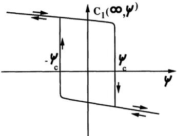
In the bizarre nonlinear phenomenology, one can also come across aerodynamic hysteresis, such as that which affect the rolling moment coefficient versus the angle of sideslip on Figure 1-1. This demonstrates that aerodynamic coefficients also depend on the past history of the flow.

These are some of the difficulties and delights of flight dynamics at high angles of attack. They are just intended to give an idea of the complexity and variety of the phenomena to be included in models. As a matter of fact, in recent computationnal surveys, aerodynamic models were taken into account in the form of tabular data. Once a proper aerodynamic model has been included in the equations of motion, specific methods have to be applied in order to analyze the fully nonlinear system.

Figure 1-1: Aerodynamic hysteresis on the rolling moment coefficient The key method is the bifurcation theory.

1.1.4

The bifurcation theory, a new powerful tool in

non-linear flight dynamics

Bifurcation theory itself is far from being new since it was invented first by Poincare at the late nineteenth century. Hopf, in the forties, and Thom [14] have also been great contributors, among others. However, the application of bifurcation theory to issues in flight dynamics is fairly recent and has been pioneered in the early eighties

by Guicheteau [15], Mehra [16, 17] and Schy [18, 19, 20].

The first success of bifurcation theory was to give an account for the aforemen-tioned old cross-coupling problem [15, 18]. This approach mainly consists in comput-ing the value of the equilibrium states1 of the system constituted by the equations of motion when one or more parameter (typically, the ailerons, the rudder or the elevator deflection) is varied. Thus, for example, one can easily obtain the equilibrium roll-rate for any combination of the control surfaces deflections. These equilibrium surfaces allow a great deal of prediction since they tell which equilibrium state the dynamic system is to be attracted to. Based on this kind of analysis, cross-coupling phenomena

1 _{An equlibrium state of a differential system i = f(s) is a state where i = 0. A linear system}

has only one equilibrium state, which is zero, but a nonlinear system may have many nontrivial equilibrium states.

such as auto-rotationnal rolling were interpreted as "jumps" or "catastrophes". The same type of approach has been applied to the more complex problem of high angle of attack dynamics [15, 17, 16, 20, 21, 22, 23] and noticeable results such as spin departure prediction have been obtained.

1.2

Statement of purpose

Nevertheless, in all these articles, fully nonlinear equations and aerodynamic datas from wind tunnel are used. Thus, sophisticated mathematical methods, so-called continuation methods, are needed, in addition to the bifurcation theory itself, to compute the various equilibrium states and their stability. This is beyond the scope of this thesis, and, consequently, a simpler model has been used in this study, one in which aerodynamic nonlinearities are included in the form of polynomials with constant coefficients. This simplification allows straightforward computations with a software specialized in polynomial processing such as Matlab but preserves the variety of all the nonlinear phenomena. Another advantage of this simpler aerodynamic model is that it allows parametric studies along with a more thorough understanding of the phenomena.

Thus, based on this nonlinear but simple model, this thesis presents a bifurcation analysis of the longitudinal and lateral dynamics of a fighter aircraft. Some strategies to control nonlinear phenomena in the largest possible range of the control deflections are investigated.

1.3

Organization of the report

This thesis is divided into four chapters, including this introduction aimed at pro-viding a historical background for bifurcation analysis applied to flight dynamics. Chapter 2 is dedicated to an introduction to the bifurcation theory itself and pro-vides the necessary tools to analyze linear and nonlinear systems. The first purpose of Chapter 2 is to make clear when a nonlinear system can be validly approximated by

its linearized system. The answer is: always, for small perturbations about an equilib-rium point, except when the jacobian matrix of the nonlinear system has eigenvalues with zero real parts. Then, Chapter 2 answers the question: "what happen when there is a zero eigenvalue?" through the center manifold theorem and the bifurcation theory, which specifically deals with system dependence on one (or more) parameter. Chapter 3 is the application of these tools to the study of the longitudinal and lateral dynamics of a fighter airplane. Nonlinear phenomena such as jumps and limit cycles are identified and analyzed through the bifurcation theory and confirmed by numerical simulations on complete differential systems.

Chapter 4 investigates some hints given in the aforementioned articles in order to provide efficient control of nonlinear phenomena. The bifurcation theory is applied to design original control laws coupling the rudder and the ailerons to avoid jumps.

Chapter 2

Introduction to the Bifurcation

Theory

2.1

Introduction

In many physical situations, a model including a system of coupled ordinary nonlinear equations arises naturally.

This is the case in flight dynamics, where the equations of motion of a rigid airplane can be symbolically written as

. = f(z), (2.1)

where f : R -- R" is a smooth function of the state vector x.

The stability1 of such a dynamical system is obviously a crucial issue. This prob-lem was originally discussed by Henri Poincar' and by Liapunov. They related the stability of system 2.1 about the equilibrium point x0 to that of the linearized sys-tem 2.2

= Df (o)C, (2.2)

1

By stability, it is meant here local stability. Given an equilibrium point z = 0o, i(ao) = 0, this

point is said to be locally stable if any trajectory in a neighborhood of zo at t = tl remains in this neighborhood at t > tl. The equilibrium point zo is asynptotically stable if, furthermore, x(t) goes to mo when t goes to infinity.

where Df(xo) is the Jacobian matrix of f, computed in xo. Thus, to begin with, it seems important to review some features about linear systems. Then, a modern ver-sion of Poincar6-Liapunov's theory is explained. It appears that phenomena specific to nonlinear equations arise only when a real eigenvalue of the Jacobian matrix is zero or when the real part of a pair of complex conjugate eigenvalues is zero. A new theory is thus needed to adress this case, whose basis is the so-called Center Manifold

Theorem. Eventually, after these necessary preliminaries, the bifurcation theory itself is exposed.

There are many textbooks dealing with the basics of linear systems, such as [24]. The theory of nonlinear systems is still under the scope of current research. A com-prehensive introduction, written to the intention of engineers and including a very large bibliography is that by Holmes and Guckenheimer [25].

2.2

The linear system x = Ax

2.2.1

General theory

A linear system is defined by

S= Az,z(O) = zo (2.3)

where A is n x n matrix with constant real coefficients and x E Rn_{. For this system,}

the only equilibrium point is x = 0. Since the solution of this system can be written

as

x(t) = zoeAt, _(2.4)

the stability of this equilibrium depends on the sign of the eigenvalues of the matrix A in the following way:

Theorem 1 The equilibrium point 0 of system 2.3 is unique and is stable if and only

Figure 2-1: Stable node (left) and unstable node

2.2.2

The two dimensional case

The two dimensional case is of some importance because it allows to represents either a first order system with two variables such as

ii = a11x + a1 2x2 (2.5)

i2 = a_{2 1}X1 + a2 2X2,

either a second order phenomenon with one variable such as

. = a~i + bx + c, (2.6)

which can be put in the form of system 2.5 by letting x = x1 and , = X2.

If A is a 2 x 2 real valued matrix, the different types of equilibria can be classified in terms of the sign of the two eigenvalues A and A2 of the matrix A.

A1 and A2 are non zero, real, distinct and of same sign

The equilibrium point is called a node, stable if A1 and A2 are negative and unstable if

A1 and A2 are positive. The aspect of the trajectories near the equilibrium point can

be represented in the phase plane, which is the plane (x, ~). In this case the so-called phase portrait looks like that represented on Figure 2-1. On this figure, the arrows denote the direction of increasing time. It can be also noticed that the trajectories

dx/dt

Figure 2-2: Saddle

approach the equilibrium point along two specific directions, which are nothing but the eigenvectors of the matrix A. This fact is of great importance and is discussed

later under the notion of invariant subspaces.

A1 and A2 are non zero, real, distinct and of opposite sign

The equilibrium point is now called a saddle and is unstable. The phase portrait near the equilibrium point looks like that represented on Figure 2-2.

A1 and A2 are non zero, real and equal

Two subcases arise in this case. If the matrix A can be put in a diagonal form then the origin can be approached or left in all directions. This is due to the fact that such a matrix is equivalent to identity matrix, implying that every non zero vector is an eigenvector. In this case, the equilibrium point is called a proper node.

If the matrix A can not be put in a diagonal form then the origin can be approached

in only one direction, due to the fact that, in this case, there is only one eigenvector. The equilibrium point is called an improper node. The phase portrait in these two cases is sketched on Figure 2-3.

:1

dx/dt

A:

I-Figure 2-3: Proper node (left) and improper node

dx/dt

Figure 2-4: Vortex

A1 and A2 are complex conjugate and have zero real part

The equilibrium point is called a center or vortez. In this case, the equilibrium is stable but not asynptotically stable. The phase portrait is sketched on Figure 2-4.

A1 and A2 are complex conjugate and have non zero real part

The equilibrium point is a focus or a spiral point. It is stable if the real part of A) and

A2 is negative and unstable if the real part is positive. These two cases are sketched on Figure 2-5. This ends the zoology of all the possible types of equlibrium in the two dimensional case. Before dealing with the nonlinear case, some definitions are needed and a section is to be devoted to the study of the notion of invariant spaces.

dx/dt

Figure 2-5: Stable focus (left) and unstable focus

2.3

Invariant spaces

In the previous schemes of two dimensional flows near their equilibrium point, it has been noted that the trajectories approached the equilibrium point along special directions, at least in the case of real eigenvalues. These directions are the eigenvectors of the matrix A. These eigenvectors are said to be invariant under the flow of A. This means that a solution of system 2.3 with an eigenvector as an initial condition remains on this eigenvector. The proof of this fact can be stated as follows:

If vi is an eigenvector of A with a real eigenvalue Ai, then Av; = Aivi. If vi is the initial condition, then the solution of system 2.3 writes z(t) = etAv,. But

t2_A2

etA [1 + tA + + ...]vi = vi + tAiv + ... = et 'vi. (2.7)

Thus, the solution does remain in the vi direction.

If Ai _{and Xi are two complex conjugate eigenvalues with eigenvectors vi and v?,}

then v_i and v? are no more invariant separatly i.e. a trajectory whose initial condition is on v_i or v? does not remain on v! or v?. Nevertheless, what remains true is that a trajectory whose inital condition is in the plane spanned by vf and v? remains in this plane. So, the plane itself is invariant. Thus, one can define the more general concept of invariant subspace.

x dx/dt

Definition 1 The subspace spanned by the eigenvectors whose eigenvalues have a

negative real part is called the stable subspace and is denoted E8, the subspace spanned by the eigenvectors whose eigenvalues have a positive real part is called the unstable subspace and is denoted Eu, the subspace spanned by the eigenvectors whose

eigen-values have a zero real part is called the center subspace and is denoted Ec. On a

stable subspace, the solutions decay, on an unstable subspace, the solutions increase, on a center subspace, the solutions either oscillate or remain constant.

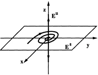
To finish with, the following example [25], which features a three dimensional flow, illustrates explicitly this concept of invariant subspaces. The matrix

-1 -1 0

A= 1 -1 0 (2.8)

0 0 2

has the eigenvalues {2, - , -i} and the invariant subspaces E" = span{(l, 0, 0), (1, 1, 0)},

E" = {(0, 0, 1)} and Ec = and the phase portrait near the origin can be represented

as sketched on Figure 2-6. On this example, one can see that a solution beginning in the plane E" = span((1, 0, 0), (1, 1, 0)} will remain in this plane although each of the eigenvectors (1,0,0) and (1,1,0) is not invariant separatly since the typical trajectory in E8 is a spiral.

This notion of invariant space is very efficient to analyze the flow in multiple dimension cases and is to be extended in the next section to the case of nonlinear systems under the notion of stable, unstable or center manifolds.

2.4

_{The nonlinear system i = f(x)}

It is now possible to come back to the nonlinear system

Eu

Figure 2-6: Invariant subspaces for matrix A

where x E Rn and f is a smooth function. Our purpose is still to inquire about the stability of the equilibria of this system. The first difference with linear systems is

that nonlinear systems can exhibit multiple equilibrium points and a good start in studying system 2.9 is to find its zeros or equilibria or stationnary solutions. These equilbria are denoted t. Then, one can linearize the system 2.9 in the following way:

c

where C

e

The question is then: how are the stability of the nonlinear system 2.9 and that of the linearized system 2.10 related?

The Poincarb-Liapunov's theory just gives the answer: the linearized system 2.10 describes properly the behavior of the nonlinear system 2.9 in the neighborhood of an equilibrium point 5 if the jacobian matrix Df(F) has no zero eigenvalue or eigenvalue with zero real part.

2.4.1

The non degenerate equilibrium case

To state a modern version of this theorem, some more definitions are needed.

Definition 2 When the jacobian matriz Df(0) has no zero eigenvalue or eigenvalue with zero real part, the equilibrium point c is said to be a hyperbolic or non degenerate equilibrium point.

Furthermore, the locally stable and unstable manifolds of t, WI andW,", are defined in the following way:

Definition 3 If U C Rn is a neighborhood of the fized point i and Ot(xo) is a solution

of system 2.9 equal to xo at t = 0, then

WoC = {xo E U I qt(zo) -+ t as t -- oo and 4t(xo) E U for all t > 0},

and

Wu. = {xo E U I bt(xo) -42 as t -- -oo and t(o) E U for all t < 0}.

WA, and Wu,, are analog to Es and EU in the linear case. It is now possible to state

a version of the Poincar-Liapunov's theorem in term of these definitions. This one is due to Hartman and Grobman (1981) and is quoted in [25, p. 13-14].

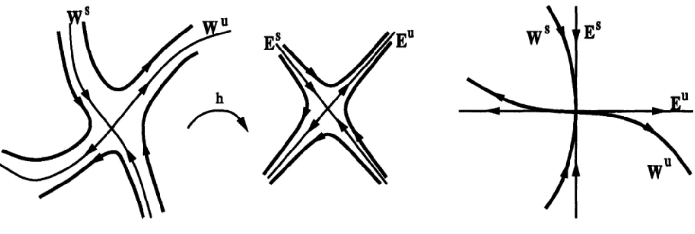
Theorem 2 If Df() has no zero or purely imaginary eigenvalues, then

a. there is a homeomorphism h defined on some neighborhood U of t in Rn locally

taking solutions of the nonlinear system 2.9 to those of the linearized system 2.10. The homeomorphism preserves the sense of the solutions.

b. there exist local stable and unstable manifolds W,, and WU, of the same di-0

mension n, and nu as those of the subspaces Es and EU of the linearized system 2.10

and tangent to E° and E" at f. Further, Wol* and W," are as smooth as f.

In other words, in the neighborhood of an hyperbolic equilibrium point, the solutions and the stable and unstable manifolds are just distorted but the stability of the equi-librium point remains the same as in the linearized case. This concept is illustrated on Figure 2-7. Thus, in the case of an hyperbolic equilibrium point, the situation is simple. Nevertheless, a question has been left unanswered: what happen when a zero or purely imaginary eigenvalue occurs?

h

W

Figure 2-7: Nonlinear and linearized flow near an hyperbolic equilibrium point (left). Stable and unstable manifolds and subspaces

2.4.2

The degenerate equilibrium case

First of all, some other techniques can be used to inquire about the stability of any kind of fixed point. Thus, for example, if a continuous and positive function which decays along any trajectory in the neighborhood of the fixed point can be found, then this point is asynptotically stable. This function is called a Liapunov function. Typically, energy is a good candidate for a mechanical system.

Another interesting technique, which is going to be described in further details in the following section, is to find out what is the behaviour of the dynamical system in the so-called center manifold.

2.5

Center manifolds and the center manifold

the-orem

Definition 4 A center manifold is defined as an invariant manifold tangent to the

center subspace.

The center manifold theorem states that such a center manifold exist but need not be unique [25, p. 127]

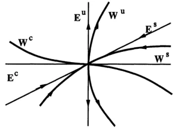
Eu

Ec

Figure 2-8: Stable, unstable and center manifolds and subspaces

the origin (f(0) = 0) and let A = _{Df(0). Divide the spectrum of A into three parts,}

,, , and o-c with

< 0 if A EO,,

ReA > 0 if Ae aO,

= 0 if AEa,.

Let the eigenspaces of a,, o- and oa be Es, EU and Ec. Then, it exists C' stable

and unstable manifolds W, and W,~~ tangent to Es and Eu (this was already stated

in the previous theorem) and a C'- 1 _{center manifold W}c _{tangent to E' at 0. The}

manifolds Ws, Wu and Wc are all invariant under the flow of f. The stable and

unstable manifolds are unique but Wc need not be unique.

The content of the center manifold theorem can be illustrated on Figure 2-8, where a center manifold tangent to the center eigenspace can be drawn but where no direction can be assigned to the flow. Thus, through the center manifold theorem, one can learn about the existence of the center manifolds but is still unable to say something about the stability of the flow in this manifold. This question is to be adressed in the next section.

--- Imftft

2.6

Stability of center manifolds

The method proposed in [25, p. 130-138] consits in projecting the flow on the center manifold and in giving an approximate expression of this projected flow by a power series expansion.

Thus, the flow near an equilibrium point can be seen to be topologically equivalent to

=

where (i, , 2) E W' x Ws x W". If one can compute

f,

stability of the center manifold.

Assuming that the unstable manifold is empty, one can put the initial system 2.9 in the following form

S= B +

f(

y = Cy+g(, y),

where B and C are n x n and m x m diagonal matrices with eigenvalues having respectively zero and negative real parts. If we assume also that the equilibrium point is 0 then f and g and their first partial derivatives vanish at the origin.

The crucial point of the method is that W can be represented as a graph near the origin, since it is tangent to the center subspace Ec. Thus,

WC _{= {(x, y)} I y = h()}, with h(O) = Dh(O) = 0. Thus, = Dh(x)i = Dh(x)[Bx + f(z, h(x))] = Ch(x) + g(x, h(x)) or A(h(x)) = Dh(x)[Bx + f (x, h(x))] - Ch(x) - g(x, h(x)) = 0

with the boundary conditions

h(o) = Dh(O) = 0.

If this partial differential equation for h cannot be solved exactly in the general case, a solution for h can be sought in the form of a series expansion. The following example illustrates this method. consider the system

u= v

i = -v + au

+3u.

This system has a single fixed point (0,0). The linear part of this system has 0 and - 1 eigenvalues. Putting it in diagonal form, one can come up with the following system, analog to 2.11,

S= a(X + y)2- (Xy+y 2 ₎

S=- - -a(aX + y)2 +(ay + y2).

Setting h(x) = ax2 + bx- + ... and computing A(h(x)), one can determine that

h(x) = -a2 + a(4afl)x3 + O(x4), (2.13)

and so that

S=

Thus, when a > 0, the center manifold is stable for x < 0 and unstable for x > 0,

/r

I

I

W

Figure 2-9: Local phase portrait and center manifold for system 2.12 and a > 0

2.7

Bifurcation theory

2.7.1

Introduction

Another class of problems to which center manifold theorem is likely to be applied is the case of sytems depending on a parameter, such as

x = f,(I), (2.15)

where xz Rn, /t E R and f, is smooth. The number of fixed points and their nature

depends on the value of /t. The point (Xo, o0) at which these changes occur is called a bifurcation point and these changes occur through a real eigenvalue or the real part of a complex conjugate eigenvalue becoming zero.

2.7.2

Basic bifurcation models

There are four types of bifurcations for one dimensional parameters. They are de-scribed by the following equations:

i = A - X2 (Saddle-node), = ILX - 2 (Transcritical),

- stable

... unstable

mu

Figure 2-10: Bifurcation diagram for the saddle-node bifurcation

x

...*** mu

.... - stable

... unstable

Figure 2-11: Bifurcation diagram for the transcritical bifurcation and

{

X + Y(A - (W2 + y'))

For each of these equations, one can draw a bifurcation diagram, which shows the number and the stability of the fixed points versus the value of the parameter p. The four bifurcation diagrams are sketched on Figures 2-10 trough 2-13. These four systems are one or two dimensional but, through the center manifold theorem, one can reduce the study of a multi-dimensional system whose Jacobian matrix has a zero eigenvalue or a pair of purely imaginary eigenvalues at (Xo, o) to that of its projection onto a center manifold. Thus bifurcations of multi-dimensional systems

mu mu

.- stabk

Gas _{... unstable}

Figure 2-12: Bifurcation diagrams for the subcritical (left) and supercritical pitchfork bifurcation

- stable

... unstable

mu

can be compared with the previous four basic types. An example of this reduction for a parametrized system is helpful.

Consider the system

U = v

v = pu- u2 -v, (2.16)

where 3 is a small variable parameter. At / = 0, the linearized system has 0 and

-1 eigenvalues at (u,v) = (0,0), with eigenvectors (1,0) and (1,-1). These two

eigenvectors are a new frame in which the system 2.16 can be re-written as

3 = (+ y)-(X + y),

S= -y - ( + y) + (X + y)2 . (2.17)

A center manifold can now be sought in the form

y = h(x,,) = ax2 _{+ bxp + c#}2 _{+ 0(3), (2.18)}

where 0(3) means third order terms in x and P. After little algebra, whose details can be found in [25, p. 135], one can find that

y = (X2 - x) + 0(3) (2.19)

and that, in this two-dimensional center manifold,

a = /(1 - ,)z - (1 - P) 2 + 0(3). (2.20)

This system can now be seen to be analog to the model of the transcritical bifurcation

. = Yx - 22, whose bifurcation diagram is sketched on Figure 2-11. The center

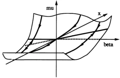
mu

beta

Figure 2-14: Two-dimensional center manifold for system 2.17

The conditions under which each of the four types of bifurcation occurs in multi-dimensional systems are now to be precised.

2.7.3

Saddle-node, transcritical and pitchfork bifurcations

Application of the center manifold reduction

It is now assumed that the system 2.15 has a zero real eigenvalue at (xo,1 o). This eigenvalue is also supposed to be simple: no other zero eigenvalue or pure imaginary eigenvalue occurs at (xo, io). Thus, one can figure out that, like in the previous example 2.16, it is possible to find a two-dimensional center manifold, in which the

system 2.15 can be reduced to X =

f1,((),

single zero eigenvalue is common to the first three types of bifurcation (saddle-node, transcritical and pitchfork) and one would now like to discriminate between these three possible cases. The answer is given in terms of the values of the coefficients of the series expansion of I with respect to F and p.

For the saddle-node bifurcation as well as for the transcritical and pitchfork bi-furcations, the zero real eigenvalue assumption implies that (Of 0

/O)(zo)

specifically for the saddle-node case, one has (8f,,0/0)(xo)

#

by the implicit function theorem that the curve of equilibria is tangent to the line

equilibria lies to one side of the line p = ito. Eventually, there is a quadratic tangency

with pt = ito and, therefore, the local phase portrait of the original system 2.15 is topologically equivalent to that of a family = ±(it - to)

+

The transcritical bifurcation is likely to occur in families where 0 is constrained to be a fixed point for any y: Vp E R, f,(Z) = 0. Thus, the hypothesis that (Of,o /ip)(Zo) 7 0 is no more valid and has to be replaced by (92f.0/&i(1)(Xo)

#

f,(-i)

0/a 2 )(xo) Z 0 is not valid and has to be replaced by

(0a3o

/4i3)(o)

0.

For a pitchfork bifurcation, one can see that the sign of (83fo 0/O 3)(xo) determines

the stability and the direction of the bifurcation branches. If ( 3fM0 /O53)(zo) is

negative, then the bifurcation is said to be supercritical. The non-zero branches are stable and occur above the bifurcation value io0. If (83f 0/& 3)(xo) is positive, then

the bifurcation is subcritical. These two kinds of pitchfork bifurcation are sketched on Figure 2-12.

Another theorem

This discrimination among the three kinds of bifurcation admitting a zero real eigen-value was based on the process of reducing the problem to a family of one dimensional

curves f,() in the center manifold. Then, the hypothesis were made on Af.

Actu-ally, a theorem can be stated which does not make use of this reduction process and whose hypothesis are done directly on the original system 2.15. Thus, for example, the following theorem can be stated for a saddle-node bifurcation:

Theorem 4 -If the original multi-dimensional system 2.15 depends on a single

pa-rameter pt and has a fixed point (xo, tPo),

-if, at (zo, to), the linearized system Df,,o has a simple zero real eigenvalue with

right eigenvector v and left eigenvector w,

-if w((Of,A/8O)(xo, 1to)

#

then (Xo, Po) is a saddle-node bifurcation point and the phase portrait is equivalent to that of Figure 2-10.

A more precise statement of this theorem appears in [25, p. 148]. Similar theorems can be formulated for pitchfork and transcritical bifurcations.

2.7.4

Hopf bifurcation

The last type of bifurcation is the Hopf bifurcation, which occurs when, at a fixed point (zo, Po), the linearized system Df,, has a simple pair of pure imaginary eigen-values. A similar but a little more complicated reduction process (which makes use of the so-called normal form theorem [25, p. 138-145]) leads to a system which can be expressed in polar coordinates as

r = (ap + br2)r

9 = c+di+er. (2.21)

If a and b are non zero, then r = lay/b|1/2 _{is the radius of a periodic orbit with}

0 = cste. This family of periodic orbits is obviously invariant and is tangent to

the center subspace in (xo, Po), thus constituting a three-dimensional center manifold passing through (xo, Io). The periodic orbits can be either stable or repelling, thus yielding subcritical or supercrtical bifurcations. The periodic orbits are also called limit cycles. The bifurcation diagram is sketched on Figure 2-13.

Chapter 3

Bifurcation Analysis of the

Longitudinal and Lateral

Dynamics of a fighter Aircraft

3.1

Introduction

The purpose of this chapter is to show how the bifurcation theory can be applied to dynamical systems in flight dynamics. An introductory example features an airplane model in a wind tunnel. It can be represented by a second order and one variable equation and has only one non-linearity. This non-linearity is due to the introduction of a nonlinear aerodynamic moment. This system exhibits a saddle node bifurca-tion. The main example features the equations of motion of an airplane in which an aerodynamic nonlinearity was also introduced. The system is of first order with five variables. Three control parameters, the aerodynamic controls provided by the

ailerons, the rudder and the elevator are also present. Their combination is responsi-ble for a wide variety of phenomena. On the various equilibrium diagrams presented below, saddle-nodes, pitchforks and Hopf bifurcations are present.

C.G.

Figure 3-1: Geometry and notations for the airplane model

3.2

Introductory example: an airplane model in

a wind tunnel

3.2.1

Description and equations of motion

In this example, an airplane model is placed in a wind tunnel. The model has only one degree of freedom, the angle of attack, since it can only rotate about a transversal axis passing through its center of gravity. On this model, the elevator is mobile and its deflection is measured by Se. This deflection is negative when the trailing edge of the elevator is up. The angle of attack is denoted a and is positive nose up. The geometry and the notations are represented on Figure 3-1. For a given elevator deflection Se, the equation of the motion about the transversal axis can be written as

I' = M + M6eSe, (3.1)

where M is the aerodynamic moment due to the whole airplane except the elevator and Ms,e is the aerodynamic moment due to the elevator. I is the moment of inertia about the transversal axis. Due to the fact that the transversal axis goes through the center of mass, there is no moment due to the weight of the aircraft.

Classically, M depends linearly on both a and & and can be written as

Mi,,,ear = 2pSIV2(Cmca + Cm~), (3.2)

where S and I are a reference surface and a reference length, p the air density, V the airspeed at infinity and where the coefficients Cma and Cma are constant.

25

2

0

Figure 3-2: Linear and nonlinear aerodynamic moments

Nevertheless, at high angle of attack, this assumption that M is linear with a and

& does not remain true and one has to introduce some non-linearities in aerodynamics.

In the real world, these aerodynamic nonlinearities are many, as it was stated in the Introduction. In this example, only the most simple non-linearity is introduced, a dependance of Cm in a2. Thus, the nonlinear form of the aerodynamic moment is

Mninea,,,, = -pSV 2(Cm,aC + Cmaa,

2

Upon substituting the expression of Mnonine,r into the equation of motion 3.1, one

obtains

Ia = 2pSV2(CM a + Cmoaa2 + Cma& + Cma₆ e), (3.4)

which can be rewritten as

a = ma + m,,a 2 + m&& + m6,6e, (3.5)

where ma, maa, ma and m6, are dimensional coefficients. The linear and non-linear "moments" mca and ma + maa,,a 2 are sketched on Figure 3-2, for mc = -10 and maa = 1.8. In this example m& and me, are also taken respectively equal to -0.25 and -30. Since m., is much smaller than ma, the linear and non-linear moments remain close to each other, but this slight difference is going to induce radical changes in the equilibrium of the model. The new equation of motion 3.5 is a second order equation

which can be rewritten as a first order system with two variables by letting x1 = a

and X2 = &. Then, equation 3.5 becomes

S= 22

i2 = macl + ma,,x + maX2 + m6ee. (3.6)

3.2.2

Equilibrium points

In the linear case (ma, = 0), there is a unique equilibrium point, regardless of the

value of the elevator deflection. This equilibrium point is characterized by

n

t-- _ m e, An = 0. (3.7)

M_a

The Jacobian matrix associated with this linear case is

Dfi= [ 0

1

The characteristic polynomial of this matrix is

A2 _ m6A - m = 0. (3.9)

The sum of the two eigenvalues is me and their product is -m,. As me, and ma are both negative, the two eigenvalues are also both negative and the equilibrium point is a stable node.

In the nonlinear case, there are one, two or no equilibrium points, which is the first significant difference with the linear case: beyond a certain value of the elevator deflection, there are no more equilibrium points. This lower value of 6e is given by the discriminant of

00 2- + 41 - A 2 0 0.2 04 0.6 0.8 1 do

At this point,

Figure 3-3: Bifurcation diagram for the airplane model. Equilibria marked with 'o' are unstable.

becoming zero i.e. for the value

2

6e = 6e

(3.11)

b e = 4mcr m6e'

At this point,

1 = Tsf = - ma (3.12)

and the point (lbif, z2 = 0, ebif) is a bifurcation point. The upper branch of

equi-libria is unstable, the lower branch is stable and tangent to the equilibrium curve of the linear case. The bifurcation diagram is sketched on Figure 3-3.

The main purpose of this example was to show how even a slight nonlinear per-turbation of an aerodynamic moment can modify the nature of the behavior of an airplane. As a matter of fact, one can see on Figure 3-3 that the stable equilibrium points in the linear and nonlinear cases remain close from each other when they both exist and that the disappearance of the nonlinear equilibrium point is very sudden.