Automated Image Analysis for NRC-IOT's Marine Icing Monitoring System and Impact Module

(1)

Publisher’s version / Version de l'éditeur:

Student Report, 2010

READ THESE TERMS AND CONDITIONS CAREFULLY BEFORE USING THIS WEBSITE. https://nrc-publications.canada.ca/eng/copyright

Vous avez des questions? Nous pouvons vous aider. Pour communiquer directement avec un auteur, consultez la première page de la revue dans laquelle son article a été publié afin de trouver ses coordonnées. Si vous n’arrivez pas à les repérer, communiquez avec nous à PublicationsArchive-ArchivesPublications@nrc-cnrc.gc.ca.

Questions? Contact the NRC Publications Archive team at

PublicationsArchive-ArchivesPublications@nrc-cnrc.gc.ca. If you wish to email the authors directly, please see the first page of the publication for their contact information.

NRC Publications Archive

Archives des publications du CNRC

For the publisher’s version, please access the DOI link below./ Pour consulter la version de l’éditeur, utilisez le lien DOI ci-dessous.

https://doi.org/10.4224/20001143

Access and use of this website and the material on it are subject to the Terms and Conditions set forth at

Automated Image Analysis for NRC-IOT's Marine Icing Monitoring

System and Impact Module

Groves, Joshua

https://publications-cnrc.canada.ca/fra/droits

L’accès à ce site Web et l’utilisation de son contenu sont assujettis aux conditions présentées dans le site LISEZ CES CONDITIONS ATTENTIVEMENT AVANT D’UTILISER CE SITE WEB.

NRC Publications Record / Notice d'Archives des publications de CNRC:

https://nrc-publications.canada.ca/eng/view/object/?id=88d88087-4db8-4db8-bb1e-c3326b960e83 https://publications-cnrc.canada.ca/fra/voir/objet/?id=88d88087-4db8-4db8-bb1e-c3326b960e83

(2)

DOCUMENTATION PAGE

REPORT NUMBER NRC REPORT NUMBER DATE

SR-2010-06 April 2010

REPORT SECURITY CLASSIFICATION DISTRIBUTION

Unclassified Unlimited

TITLE

Automated Image Analysis for NRC-IOT’s Marine Icing Monitoring System and Impact Module AUTHOR(S)

Joshua Groves

CORPORATE AUTHOR(S) / PERFORMING AGENCY(S)

PUBLICATION

SPONSORING AGENCY(S)

IOT PROJECT NUMBER NRC FILE NUMBER

42_2279_16

KEY WORDS PAGES FIGS. TABLES

Image Analysis, Marine Icing, Marine Icing Monitoring System, Data Extractor for Marine Icing Images, Impact Module, Impact Module Image Processor

79 27 0

SUMMARY

National Research Council’s Institute for Ocean Technology (NRC-IOT) has successfully applied image processing and data extraction techniques to measure structures and objects in images. This plays a key role in two major projects; IOT’s Marine Icing Monitoring System (MIMS) and Impact Module. By use of software developed at IOT, researchers are able to analyze ice accumulation remotely through cameras for MIMS, thus creating an automated warning system to identify hazardous icing events. Researchers are able to apply similar software to images captured by IOT’s Impact Module, to analyze pressure distribution for impacts. The impact module will be able to be mounted on vessels in the future for bergy bit trials, allowing for research of bergy bit collisions with vessels to occur. Image processing and data extraction has been proven to work effectively for both IOT’s Marine Icing Monitoring System and Impact Module, and will be used greatly in future analysis.

ADDRESS

National Research Council Institute for Ocean Technology Arctic Avenue, P.O.Box 12093 St. John’s, NL A1B 3T5

(3)

National Research Council Canada

Institute for Ocean Technology

Conseil national de recherches Canada

Institut des technologies océanique

Automated Image Analysis for NRC-IOT’s

Marine Icing Monitoring System and Impact Module

SR-2010-06 Joshua Groves April 23, 2010

(4)

List of Figures

1 MIMS components . . . 3

2 MIMS cameras mounted on upper deck rail of vessel . . . 3

a Starboard Camera . . . 3

b Port Camera . . . 3

3 Samples of MIMS Images Captured While Deployed on the Atlantic Eagle . . . 5

a Sea Spray . . . 5

b Water on Deck . . . 5

c Snow on Deck . . . 5

d Ice Covered Camera Window . . . 5

e Ice on Vessel . . . 5

4 Bruce’s process and sample output graph . . . 7

a Processing Steps . . . 7

b Sample Graph for Bruce’s Results . . . 7

5 Bruce’s Analysis Positions . . . 7

6 Li’s Sample Average Intensities Plot for a Processed Image . . . 8

7 Li’s Output for Two Positions . . . 9

a Original Pole . . . 9

b Sample Output Image for Pole . . . 9

c Output Graph for Pole . . . 9

d Original Ellipse . . . 9

e Sample Output Image for Ellipse . . . 9

f Output Graph for Ellipse . . . 9

8 DEMII Image Processing, Rotated/Cropped . . . 10

9 DEMII Image Processing, Anisotropic Diffusion . . . 11

10 DEMII Image Processing, Sobel Edge Detection . . . 11

11 DEMII Image Processing, Vertical Grey Erosion and Dilation . . . 11

12 DEMII Image Processing, Binary Threshold . . . 12

13 DEMII Image Processing, Custom Noise Reduction and Vertical Binary Dilation . . . 13

14 DEMII Interface, Main Window . . . 14

15 DEMII Interface, Settings Window . . . 17

16 Manual/DEMII/Li’s Results Compared for a Structure . . . 18

17 Graph of DEMII Results for Sample Positions . . . 19

a Graph for Sample Pole Position . . . 19

(6)

18 DEMII Compilation Image for Sample Pole Position (left: 1-21, right: 22-41) . . . 20

19 DEMII Compilation Image for Sample Rail Position (left: 1-21, right: 22-41) . . . 21

20 IOT’s Impact Module and Sensor Technology . . . 23

a Sectional View of IOT’s Impact Module . . . 23

b Sectional View of the Pressure Sensor . . . 23

c Bottom View of a Strip Under Pressure . . . 23

21 Ice Test for IOT’s Impact Module . . . 23

22 Li’s Method of Removing Support Structures . . . 24

a Original Image . . . 24

b Image with Support Structures Removed . . . 24

23 Li’s Method to Increase Measurement Precision . . . 25

a Original Image . . . 25

b Image After Linear Interpolation . . . 25

24 Li’s Image Processing Steps . . . 25

25 IMIP Sample Run . . . 28

26 Actual Load versus IMIP Measured Load (A*P) . . . 29

27 Processing Steps with IMIP for Sample Impact Module Image . . . 29

a Sample Blank Reference Image . . . 29

b Sample Image to be Processed . . . 29

c Image After Processing . . . 29

d Pressure Distribution and Magnitudes Mapped . . . 29

Appendices

Appendix A: Summaries of MIMS Observations (2007-2008, 2008-2009) Appendix B: IOT-DEMII Source Code

Appendix C: IOT-IMIP Source Code

Appendix D: Additional Development Images Appendix E: PTLens Software Configuration

(7)

1 Introduction

1.1 General Overview

With the rise of technology, researchers have taken advantage of computer processing in unforeseen ways. One of these researchers, Dr. Robert Gagnon of National Research Council - Institute for Ocean Technology (NRC-IOT), takes full advantage of computer processing with regards to image analysis using several techniques. In one of his projects, he analyzes marine icing events through an automated process in which data is collected about ice build-up on vessels. For this project, Dr. Gagnon designed the Marine Icing Monitoring System (MIMS) to research icing events on the vessel for a desired timeframe. In another project, Dr. Gagnon enables research of impact through an innovative impact module design. Both projects make use of image processing to conduct research of images that are collected by automated camera systems. The projects employ several techniques to refine and detect data that is observed through the images, in steps which are automated through computer programs. Computer programs for these projects are written in Python, an efficient programming language which enables rapid development of modern applications.

1.2 Application of Image Processing

Images collected from the Marine Icing Monitoring System (MIMS) are analyzed through edge detection tech-niques, which allows users to view data regarding the amount of ice build-up on the vessel in any image, at specific points on the deck. The settings dialog in this program allows users to adjust settings for effective use on virtually any vessel. This technology will be extended in the future to allow the MIMS to act as a warning system, to send signals when current ice build-up amount is detected to be hazardous to the vessel. In the other aforementioned project, the impact module developed by Dr. Gagnon uses a high speed camera to collect images of pressure devel-opments. These images are processed sequentially, by using a reference image to determine where pressure exists. The program uses intensities in the image to map local pressure values in great detail. This technology has many applications, and could enable researchers to analyze data with methods deemed to be previously impossible.

(8)

2 Automated Image Analysis for Marine Icing Events

2.1 Marine Icing Information

Ice accumulation is one of the greatest problems that vessels are faced with, especially in harsh conditions where rapid accumulation may occur. The freezing point of seawater is just−1.9◦_{C, due to its high salinity [7]. This}

means that freezing will occur when air temperature is below this point, and sea spray, rain, or fog cause moisture to be deposited on structures onboard the vessel. Oftentimes, sea spray contributes the highest amounts of mois-ture, and is the result of collisions between the hull of the vessel and sea waves. While vessels take measures to prevent seawater from being retained on the deck, the freezing of seawater may occur too rapidly, and ice becomes accumulated. The frozen seawater on structures of the vessel is referred to as marine ice.

The problem of marine icing events exists wherein a vast amount of ice accumulation occurs. Great amounts of ice accumulation can reduce the stability of vessels, since the center of mass for the vessel becomes shifted due to the nonuniform weight that is added. While the effects may be less noticeable with the more heterogenous ice accumulation on the vessel, such as in the case of freezing fog, it is highly noticeable for the case of sea spray. For sea spray, the majority of ice accumulation occurs on the bow of the vessel, which could potentially cause a shift in pitch. This rotation about the center of flotation of the vessel reduces stability and must be countered by a change in trim angle. However, changes in trim angle are limited, therefore this ice accumulation can often be extremely hazardous. Research on ice accumulation will allow for detailed data to be collected and analyzed, and to establish necessary warnings when ice accumulation becomes severe.

2.2 Marine Icing Monitoring System (MIMS)

2.2.1 Housing

The Marine Icing Monitoring System (MIMS) is a system designed to collect images of icing events on the vessel for data analysis. MIMS consists of two high-resolution cameras as well as a computer enclosure, telephone enclosure, and power enclosure. The devices are constantly supplied power through a 110 VAC power supply in the power enclosure, connected to the devices by power cables. MIMS is created with well-insulated, waterproof materials, which provides it with an ideal design for use in harsh sea environments. MIMS receives images from the cameras, and saves these images to its internal hard drive. The computer is connected to a telephone enclosure, which can be used as a remote control for an operator at the Institute for Ocean Technology (IOT). Since the camera images are large, MIMS creates thumbnail versions which can be streamed quickly. The operator is able to view these thumbnails through a satellite phone in the telephone enclosure. This feature therefore enables the operator to monitor MIMS to ensure that it is receiving images correctly, as well as allows for MIMS to be remotely turned off or restarted if desired. The total system weight is approximately 132 pounds, including cables, and the power consumption is approximately 250 Watts. All components are shown in Figure 1.

(9)

Marine Icing Monitoring System Components

Total system weight, including cables, is approximately 132 lb Total system power is approximately 250 Watts

200ft cable 20lb weight 16" 18" 8"

CPU Box

20 lbs weight 16" Satellite Phone Antenna 16" 14" 8" Transformer Box 20 lbs weight 110 VAC in 24 VAC out 12"

Camera Housing and Mount Aluminum or Stainless Steel

26 lbs weight

7.5"

22.5" 8"

Figure 1: MIMS components 2.2.2 Cameras

MIMS collects images at a specified time interval, from both starboard and port cameras mounted on the deck of the vessel. Currently, the cameras collect images every twelve minutes, with a six minute offset between acquisition. These images are stored on a hard drive, and are collected after the desired quantity of collection time has passed.

(a) Starboard Camera (b) Port Camera

Figure 2: MIMS cameras mounted on upper deck rail of vessel

Ice build-up or sea spray on the housing window was found to reduce visibility of the cameras. To deal with this issue, a heater was added to MIMS to ensure that the cameras were never affected by outside conditions. The heater is colorless and has high resistance, and was installed to the center of the housing window. The material is

(10)

electrified, which warms the window and effectively reduces any moisture from reducing visibility for the cameras. The cameras are shown in Figure 2.

As of now, MIMS has been used to collect data for the winter seasons for multiple years. The events of surveying six months of images, for both 2007-2008 and 2008-2009, are summarized in Appendix A. All images taken through MIMS are named based on the time at which they were taken, and the tables explain what events can be observed in each image. Through these tables, it is possible to quickly locate images that contain events of interest, such as spray images, or ice, water, and snow on the vessel. The summary tables also note when the camera visibility is reduced, due to low lighting or ice covering the window of the camera. These are important to researchers at IOT to ensure that the MIMS system can be adapted such that it will not be affected by these issues in the future. The issue of low lighting is currently being dealt with, by using higher resolution cameras with refined settings for automatic low lighting adjustments. If the window of the camera causes problems in the future, then the heater for MIMS will have to be adjusted as well. For the table, however, the event which draws most interest for MIMS is the occurrence of icing events. In these events, the various structures on the vessel become coated with ice. Through robust edge detection methods in image analysis, it is possible to calculate how much ice is observed to be present on the vessel. Therefore, from these calculations, MIMS can act as a warning system for hazardous ice build-up. Sample images captured by MIMS are shown in Figure 3 on the following page, where all images displayed are of interest to researchers at IOT for various reasons.

(11)

(a) Sea Spray (b) Water on Deck

(c) Snow on Deck (d) Ice Covered Camera Window

(e) Ice on Vessel

(12)

2.3 Previous Analysis Techniques

2.3.1 Previous Research

Several methods have been used to analyze these marine icing event images in previous years. Leah Gibling, Wayne Bruce, and Lian Li, working for the Institute for Ocean Technology have made attempts to read measure-ments from structures from the images. These attempts have proven to be successful in reading measuremeasure-ments of structures from images, and the analysis process has become very refined since the initial attempts.

2.3.2 Leah Gibling’s Method

The first method was used by Leah Gibling, to analyze images from the winter of 2006. In her analysis, she introduced a manual method of measuring ice thickness in her report “Marine Icing Events: An Analysis of Images Collected from the Marine Icing Monitoring System (MIMS).” Gibling’s method was to measure the quantity of pixels between two edges of the selected structure for each ice accumulation image. After this data is recorded, she compared the results with the image with no icing event. The difference between the two values was therefore an approximation the amount of ice on the structure. Gibling’s measurements were recorded in a Microsoft Excel spreadsheet, where they could then be graphed to show the trend of ice growth. While the measurements appeared to be accurate, it takes quite long to measure these structures manually. It was desireable to automate this process for increased speed and for future use with MIMS.

2.3.3 Wayne Bruce’s Method

After Gibling’s method was used for image analysis, Wayne Bruce created an automated analysis method by use of the technique. In his report, “Automated Image Analysis For Marine Icing Events,” Bruce created a program in Python, a programming language that was created for rapid development of software. Python has thousands of open-source modules which can be easily included in programs, such as implementations of many popular algorithms, for example. For Bruce’s program, he used the Python Imaging Library (PIL) to analyze images of marine icing events. PIL is commonly used for simple image processing. In Bruce’s method, PIL’s edge detection algorithm is used to raise and lower the intensities of edge and background pixels, respectively. By applying Gibling’s method and measuring the number of pixels between intensity peaks, Bruce was able to find measurements for the structure being analyzed.

The analysis process used by Bruce’s program can be divided into three steps. In the first step, image processing, the program rotated the image to make the selected position have vertical edges. The program then used PIL’s color enhance and then converts the image from RGB to greyscale, where a single intensity value could be extracted for each pixel in the image. Bruce’s program then cropped the selected position from the image. After this step, the program used PIL’s edge detection algorithm, which scaled the intensities of edge pixels as described above. Bruce’s method then records the position of the left and right peaks, which is where the sharpest edge is found to

(13)

have occurred. The width given by the difference of these two values was recorded. These two processing steps are outlined in the top part of Figure 4. The third step involved graphing the data points through an automated process. The program used a Python module called Matplotlib to produce a graph based on these measurements.

(a) Processing Steps (b) Sample Graph for Bruce’s Results

Figure 4: Bruce’s process and sample output graph

Figure 5: Bruce’s Analysis Positions

Automated image analysis through Python was found to be much faster than manually analyzing the images. How-ever, the measurements were shown to be less accurate through Bruce’s automatic measurements. For example, while there were 41 input images for a particular marine icing event, there were only 21 measurements plotted in the graph of Figure 4b. This means that the program automatically removed many measurements, since it was unable to detect many widths correctly. Therefore, it was necessary to refine this technique to improve it further. 2.3.4 Lian Li’s Method

To improve on Wayne Bruce’s method, Lian Li used techniques to make the edge measurements more accurate and robust. Li imported another module to the program, NumPy, which provides Python with the ability to use and manipulate arrays, as well as use some scientific algorithms on these arrays. In Li’s report, he discussed three

(14)

methods of automated edge measurement that he used to improve Bruce’s program.

For Li’s improved program, the images were pre-processed with enhancement and median filters that are included in PIL. Then, as in Bruce’s original method, the greyscaled versions of the images were rotated, cropped, and PIL edge detection was applied. The first method of measuring structure widths that Li discussed is to average the intensities at each column of the image, and to subtract the average left intensity peak location from the average right intensity peak location. Li assigned percentage values to scale these peak locations based on the structure, as he found that the actual edge was commonly a few pixels towards the middle beyond what he measured. All values that are measured are recorded and graphed for further analysis, and an output compilation image containing each analysis step is produced. An example of an average intensities plot produced by Li is shown in Figure 6. For ideal images where the only edges detected were for the structure being analyzed, there were clear peaks in intensity magnitude where the edges occurred.

Figure 6: Li’s Sample Average Intensities Plot for a Processed Image

Li also applied this method to structures other than vertical objects that were previously analyzed. For example, he found some success when analyzing an elliptical structure. To analyze this type of structure, Li’s program used a method which involved removing a piece at the object’s centerline, after it had been rotated. The program then found the maximum width of the structure that was detected, and drew points to indicate where the edges were found. Li noted that as the edge detection process yielded weak edges due to blurred or noisy images, the measurements became more uncertain.

Li then tested two alternative methods that he hypothesized. Li’s second method that he used to analyze the intensity matrix dealt with analyzing the intensities at each row of the cropped structure. In this process, the program analyzed each row and recorded the width that it found between edges. Li’s program then averaged these values to give a final width for the structure, and repeated this process for each image. The other alternative method that was used by Li to analyze structure widths, involved resizing the image to create more pixels for analysis by interpolation. By resizing the image, Li stated that he could find subpixel intensities and thus return

(15)

more precise measurements. Despite some good results with these alternative methods, they did not appear to work well on images with noisy backgrounds. As a end result, Li decided to use these methods to introduce data when his standard method failed. The program created by Li therefore had more options and was more robust than the initial automatic method introduced by Bruce. While this program worked quite well on several structures for the specific icing event that was analyzed, it had to be manually reprogrammed each time a different structure or imageset was to be analyzed. As well, it had many issues when it was used on images that were not ideal, and sometimes the program stopped running when faulty values were returned. Before being used with MIMS was possible, further refinement was required. Sample results from Li’s program for two sample positions are shown in Figure 7.

(a) Original Pole

(b) Sample Output Image for Pole

(c) Output Graph for Pole

(d) Original Ellipse

(e) Sample Output Image for Ellipse

(f) Output Graph for Ellipse

(16)

2.4 Data Extractor for Marine Icing Images (IOT-DEMII)

2.4.1 Purpose

Through research, it was found that there were several image processing techniques that could refine the program’s results. Trying to integrate these methods with the existing code proved to be a challenge, since some of the code required precise operating conditions. These operating conditions were required to be adaptable for use with MIMS. Using pieces from Li’s program’s code, a new program was created, entitled Institute for Ocean Technology’s “Data Extractor for Marine Icing Images” (IOT-DEMII). DEMII applies several techniques to ensure that the image processing step before data extraction was more robust and efficient than its predecessors.

2.4.2 Image Processing Techniques

The intial step for the program is to select and open the image, from a list of images that are part of a set. DEMII converts the image to grayscale, and then crops the structure and rotates it. It then automatically crops this rotated box, so the rotated box edge does not influence future processing steps. Since DEMII crops the image at the very start, it reduces the memory required to process the image. Both the crop co-ordinates and the angle of rotation are user-defined. This process is shown in Figure 8, where the left image is the original structure image after being cropped, and the right image is the rotated and cropped image.

Figure 8: DEMII Image Processing, Rotated/Cropped

DEMII then processes the image with an anisotropic diffusion filter. This filter is an edge-preserving blur, as described by Perona and Malik in their paper, “Scale-Space and Edge Detection Using Anisotropic Diffusion” [5]. The filter was translated to Python code from a 2D greyscale MATLAB implementation originally created by Daniel Lopes [3], so that it may be used in DEMII without any requirement for additional software. DEMII uses a conduction coefficient function for this filter that can be described by the following function:

g(∆I) = 1 1 + (||∆I||_k )2

where∆I = time step, ||∆I|| = current direction matrix, k = gradient modulus threshold

This filter replaces the median filter that was used previously. Anisotropic diffusion appears to be more ideal than the median filter. This is because it will not alter the edges that are to be extracted when the gradient modulus threshold is set to a proper value for the image, where the median filter blurred each pixel based on the intensities of its eight neighbouring pixels. The desired effect of the anistropic diffusion filter is demonstrated in Figure 9.

(17)

Figure 9: DEMII Image Processing, Anisotropic Diffusion

After the filter has been applied to the current image, DEMII uses the Sobel operator to detect the edges and alter the image to show where edges are located, by use of a Python implementation in the module SciPy [6, 2]. All strong edges are identified by high intensity values for the pixels at which they are detected, and the weak edges are identified by low intensity values. This edge mapping is similar to the edge detection technique previously used through PIL — however, the PIL edge detection algorithm is not documented and appears to yield worse results for MIMS images. The SciPy implementation of the Sobel edge detection operator is open source, and can be modified if desired. This allows DEMII to use a custom built Sobel filter if the step needs to be refined in the future, which is very advantangeous over the previous technique. The Sobel operator detects edges through approximations of the derivatives of intensity for each pixel, and appears to perform this task quite successfully, as shown below in Figure 10.

Figure 10: DEMII Image Processing, Sobel Edge Detection

Following edge detection, DEMII alters the current image through grey morphology operations. The program first erodes the image (Ioriginal) by a vertical structure of a user-defined length (V1), and then dilates the image using

another vertical structure of user-defined length (V2). Mathematically, it performs the following:

Iprocessed= (Ioriginal⊖ V1) ⊕ V2

where⊖ and ⊕ denote erosion and dilation, respectively

This operation is often synonymous to grey opening operation (I◦ V ), since the user-defined lengths for both vertical structures are commonly set to have the same value. However, DEMII allows a user to modify either of these lengths if a user desires. Sample results from the grey morphology operations are shown below in Figure 11, where it is shown that the desired vertical edge lines have been extracted successfully.

(18)

For the next step of image processing, DEMII uses a binary threshold. All values in the image that are above the threshold are assigned a binary value of one, while all other values are assigned a binary value of zero. This step is required to give all high intensity pixels equal weighting, since they are all considered to be strong edges after the previous steps have not removed them. The pixels having values less than the threshold are considered to be noise, and are therefore removed to prevent them from causing future issues in measuring the structure widths. The following equation describes the thresholding process for each row and column of the image from the previous step, and Figure 12 shows sample results of binary thresholding:

Iprocessed(r, c) =        1 if Ioriginal(r, c) > t, 0 otherwise.

where r= current row, c = current column, t = threshold value

Figure 12: DEMII Image Processing, Binary Threshold

DEMII then uses a custom noise reduction filter, which was created specifically for use with MIMS images. This filter is based on the consistency that is to be expected from neighbouring images, and the fact that ice growth is unlikely to undergo extreme amounts of growth between images. In this filter, a window is defined, which is just a square that will be used to examine pixels. Noise removal occurs by moving the window through the current image (In) for each row (r) and column (c) within the boundaries provided by the window size (w), and

comparing the selected pixels to the pixels in the neighbouring images. For the first and last image in the set, this cannot occur since they have less than two reference images to be compared to. For all other images in the set, the preceeding (In−1) and succeeding (In+1) images are compared to the current image for each window position.

In the comparison process, if all pixels in the window for the two comparison images have values of zero, and all pixels do not have values of zero for the window in the current image, then all pixels for the window in the current image are set to zero. To extend this process, every image except for the first and last image for this set are compared yet again to the images before and after the preceeding and succeeding images (In−2 and In+2),

respectively.

For the custom noise reduction filter, there are four parameters; the number of iterations through the image set for noise filtering, and the window size for noise reduction, for both steps. It shows great accuracy in removing outliers and noise from the processed image, however consideration should be taken into the amount of acceptable image shifting, since image shifting may cause valid data points to be removed if large amounts of inconsistencies occur between images.

(19)

The custom noise reduction filter can be summarized mathematically by the following statement, where∨ denotes logical disjunction: I(r − w : r + w, c − w : c + w)n= 0, if : if w X i=−w w X j=−w (I(r − w : r + w, c − w : c + w)n−1∨ I(r − w : r + w, c − w : c + w)n+1)ij= 0

when n-1 and n+1 exist and if w X i=−w w X j=−w (I(r − w : r + w, c − w : c + w)n−2∨ I(r − w : r + w, c − w : c + w)n+2)ij = 0

when n-2 and n+2 exist

After the noise reduction process, DEMII uses binary dilation with a vertical structure (V ) of user-defined length. This morphology operation is similar as described previously, but no erosion occurs in this step. This step joins any small gaps between vertical edges, and can ensure that measurements are taken from widest point of the structure when the width varies greatly between rows of the image. Expressed mathematically, this step consists of the following:

Iprocessed= Ioriginal⊕ V

Figure 13: DEMII Image Processing, Custom Noise Reduction and Vertical Binary Dilation

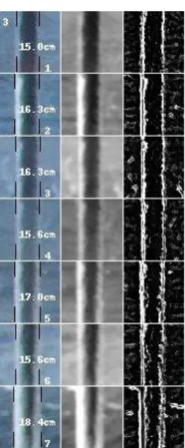
It is difficult to demonstrate the custom noise reduction filter without a set of images the filter requires to use for consistency. However, the results of the custom noise reduction filter are noticeable in sample output images in Figures 18 and 19, where unwanted pixels with intensity values were removed prior to vertical binary dilation. After vertical binary dilation, image processing is completed. The images should consist of pixels with values of one where edges are detected, and noise should be removed efficiently if the settings are adjusted properly. An example of a fully processed image is shown above, in Figure 13. DEMII is then able to easily extract data from the images in the set.

2.4.3 Data Extraction Process

For the data extraction process, DEMII analyzes each row of the binary dilated edge image. For each row, DEMII finds the leftmost and rightmost pixels that have values of one. It records the width and center of the structure for each row by recording the difference between and the average of the locations of these two active pixels, respectively. Both the differences and centers are averaged separately, to get average width and average center for

(20)

the structure. The width measurements are optionally multiplied by a calibration factor to convert widths from a pixel value to another unit, such as centimetres or inches. These values are output to DEMII’s console, and the edge positions are drawn on the original images. All measurements are saved to a comma-separated value file, and an output compilation image is saved which shows the major processing steps.

2.4.4 Usage Guide

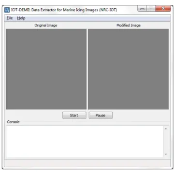
When DEMII is executed, users are presented with a window that provides a graphical user interface for processing and analyzing the images from MIMS. This interface is divided into five main “panels”, as shown in Figure 14 below.

Figure 14: DEMII Interface, Main Window

The first panel is the menu bar, which includes the following headers and subheaders: File Displays a menu with program commands.

Load Settings Load image processing settings from configuration file. Modify Settings Modify the current image processing settings.

Save Settings Save the current image processing settings to a configuration file. Image Directory Specify the path to the image directory for processing.

Clear Console Clear DEMII’s output console to prevent overflows for very large image sets. Exit Terminates the program.

(21)

The Modify Settings Dialog will be explained after all panels are discussed.

The second panel of DEMII is composed of two image panels to display scaled images that are being processed. These panels are displayed aligned horizontally such that the modified images can be easily compared to the original at each step. The panels are labelled according to this feature, and therefore they are named ‘Original Image’ and ‘Modified Image’. In the image processing stage, there are three images displayed in these panels for the current image being processed. For the first step of processing, the original cropped image and the rotat-ed/cropped image are displayed in the left and right panels, respectively. For the second step of processing, the rotated/cropped image is shifted to the left panel, while the right panel is updated with the image after the Sobel and morphological operations are applied. After the image processing has been completed, the data extraction process occurs. Images are displayed to visualize the results from this process. In the left panel, the cropped/ro-tated color image is shown again, but this time lines are drawn to indicate where the edges have been detected to occur. In the right panel, the final binary image is shown, which is the image that provides DEMII with the edge locations as shown in the left image.

DEMII’s third panel consists of two control buttons, that are used to begin, pause and resume processing. Once the start button has been clicked, it will be disabled until all images have been processed and measurements have been returned. The second button can be used to pause the program at any step, such that the user is able to view the displayed images if the image processing occurs too quickly to view normally. While DEMII is paused, clicking this button again will cause the processing to resume and continue at the current step.

The fourth panel is a text box that is used for output from each step of data processing. This can be useful to show how many images have been processed thus far, or to show the status of the program. For example, when settings are loaded from a file, this console will be updated with a message to reflect this change in settings. This eliminates any potential confusion when working with multiple configuration files.

The final panel in DEMII is the status bar. It is shown on the very bottom of the user interface, and displays messages about the current state of the program. After every major action, the status bar updates to show the user what step of the processing that DEMII is currently performing. This is useful if the user is not viewing the console in great detail, and would like an summary of the current process that is occurring.

Referring back to the Modify Settings menu button, clicking this menu results in the popup of a dialog window where the user can modify the settings for image processing, as shown in Figure 15. Each of these settings is described below, roughly in the order that they are used by DEMII. Assume that input values are to be any reasonable real number unless stated otherwise.

Image Properties settings relating to structure selection from each image

Calibation Factor which measurements are multiplied to convert from pixel units to centimetres or inches, etcetera.

(22)

Angle Angle of which the image will be rotated by. Manually adjusting this value may yield best results. Left Left column location for the crop box.

Top Top row location for the crop box. Right Right column location for the crop box. Bottom Bottom column location for the crop box.

Get Co-ordinates Opens the image specified, and allows the user to click on two positions. The first position will be used as the point for left and top co-ordinates, and the second position will be used as the point for the right and bottom co-ordinates. Clicking on the image a third time will bring the user back to the settings dialog.

Image Processing settings relating to the image processing stage

AF Iterations Number of iterations to run for anisotropic diffusion f ilter. Input should be a whole number. AF Kappa Gradient modulus threshold value for anisotropic diffusion f ilter. This value should be manually adjusted with various iteration settings, such that ideal conductance is found where the background is blurred but edges are well-defined.

GE Vertical Length Grey erosion structure length. Controls the magnitude of grey vertical erosion. Input should be a whole number.

GD Vertical Length Grey dilation structure length. Controls the magnitude of grey vertical dilation. Input should be a whole number. As this value is modified, grey erosion vertical length should be updated as well, unless the user desires to have different behaviour than a grey opening operation. Ideal values of this should extract all important lines, while discarding short lines that are not edges.

Threshold Threshold value to be used for binary thresholding. Intensity values greater than this value become ones, intensity values lower than this value become zeros.

NR Window 1 Size Noise reduction window size, used for all images in the set except for the first and last (where n-1 and n+1 exist, if n is the current image). Value is very sensitive to image shifting. Input should be a whole number.

NR Window 2 Size Noise reduction window size, used for all images in the set except for the first two and last two (where n-2 and n+2 exist, if n is the current image). Value is very sensitive to image shifting. Input should be a whole number.

NR Iterations Noise reduction iterations to perform. In most cases, this can be set to one or two for efficient noise reduction while not removing important data. Input should be a whole number.

BD Vertical Length Binary dilation structure length. Controls the magnitude of binary vertical dilation. Input should be a whole number.

(23)

Time Steps Amount of time that passes between MIMS captures images. Used for the output measurements. Delay Amount of time to pause between processing steps and displaying new images in DEMII’s image

panels. Useful if processing is too fast to view otherwise.

Apply Return to the main window storing the new values as the processing settings. This will not update the configuration file, only for the current process. The configuration file can be saved after this occurs to save any changes.

Cancel Return to the main window, discarding all modifications.

Figure 15: DEMII Interface, Settings Window

Another feature that is vital to DEMII’s use with MIMS is the support of command line arguments. If DEMII is called from the command line, three arguments can be given to specify the configuration, image directory, and exit option for automatic processing. This allows MIMS to call DEMII without requiring any manual execution. For example, the following calls demii with three arguments:

python demii.pyw "C:\config\position 1.ini" "C:\images" 1

This will cause DEMII to open the configuration file specified (“C:\config\position 1.ini”) and select the directory path for images (“C:\images”). The “1” gives DEMII the command to automatically exit after it is finished processing and the results have been saved. If this option is set to “0”, then DEMII will remain open after processing. The directory path should not have a trailing slash, and both arguments must use backslashes for the paths. Failure to follow this standard will result in program errors. As well, the first two arguments require to be enclosed in quotations, while the third argument requires only the option number. In the future, more error checking steps could be added to DEMII to ensure that user error does not prevent DEMII from running properly. These error checking steps could be applied not only to the command line arguments, but for all aspects of the program.

(24)

2.5 Analysis

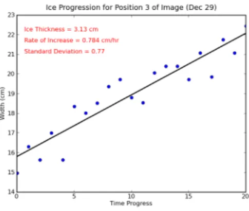
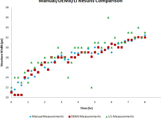
Using DEMII with images collected by MIMS proved to show great success. By comparing DEMII to Li’s program, it was found that DEMII returned results that had higher correlation with manually measured results. This means that DEMII’s new techniques perform more accurately than the techniques that were previous used. Below in Figure 16 is a graph comparing DEMII’s, Li’s, and manually measured results for a set of images.

Figure 16: Manual/DEMII/Li’s Results Compared for a Structure

DEMII was also used on other image sets to see how well it performs when various amounts of ice build-up occurs. It was found to effectively find the width of the ice accumulation on several structures. Figures 17, 18 and 19 show examples of output measurements and processed images from DEMII.

(25)

(a) Graph for Sample Pole Position

(b) Graph for Sample Rail Position

(26)

(27)

(28)

3 Automated Image Analysis for Impact Module

3.1 Impact Module Technology

Ice impact on ships that face harsh arctic conditions is a major issue. The collision of icebergs or bergy bits with vessels causes extremely high amounts of force to be transferred to a certain area of the vessel. The Titanic is one of the most famous cases in which ice impact has damaged a ship, where it was damaged by ice impact in 1902. The “unsinkable” ship struck an iceberg, and sank due to the damage caused by the collision between the iceberg and ship. Although modern ships are now built with stronger structures and can handle higher amounts of force than previous years, marine disasters due to ice impacts still occur. To research the forces applied to vessels during collisions with bergy bits, Dr. Gagnon of the National Research Council’s Institute for Ocean Technology designed an impact module to measure the ice impact forces and their distribution across the region being analyzed.

The Impact Module is comprised of several components; a sensor made up of many pressure strips, a large acrylic block, and a high-resolution camera. The pressure strips are shown in Figures 20a and 20b, where each strip has a slight curvature. They are arranged on the top of the acrylic block, and are oriented such that their curved surface will touch the face of the acrylic block. When pressure is applied to a strip, the curved surface starts to flattens and contacts the acrylic, thus creating a white region on the acrylic block. The white regions of a sample strip is shown in Figure 20c, where the width of each row of the strip is proportional to the amount of pressure applied to the strip. The sensor is covered by a thin metal sheet which protects the strips during impacts. The acrylic block is translucent, and has dimensions of one metre wide by one metre long by half a metre thick. Lights are distributed throughout the acrylic block to illuminate the regions where pressure is created. The strength of the acrylic block allows it to shield the high-resolution camera located behind it during impacts. White regions are visible by the camera in this manner, such that the camera is able to capture images of pressure distribution based on the light it receives from the regions. The camera is able to capture images at a rate of 250 pressure images per second, which gives researchers the ability to analyze collisions at any particular millisecond if so desired.

To test the feasibility of IOT’s Impact Module recording pressure distributions from bergy bit impacts, a sample ice collision test was conducted. In this test, a large block of ice was raised by crane, and moved over the center of the sensor. As the ice was released from the crane, images are captured by the camera and saved to a computer to be analyzed. The test procedure is demonstrated in Figure 21. The test was sucessful, and it was proven that the impact module can capture pressure distributions from ice collisions. Therefore, the impact module has been included in new design plans to be mounted onto a vessel and used in future bergy bit trials, as shown in Appendix D.2. The data collected from these trials will be useful to designing ships for safe operation in arctic conditions, where ice may be hazardous to ships.

(29)

(a) Sectional View of IOT’s Impact Module

(b) Sectional View of the Pressure Sensor (c) Bottom View of a Strip Under Pressure

Figure 20: IOT’s Impact Module and Sensor Technology

(30)

3.2 Previous Analysis Techniques

Lian Li’s program created for MIMS images, as discussed previously, was modified to be applied to the images captured by IOT’s Impact Module. In this modified program, edge detection is performed on each pressure strip. The difference between edge locations for each row in each strip represents a width, which is proportional to pressure applied on that row, as stated previously. The input images for this program are images that have already been processed by two additional pieces of software.

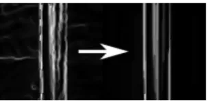
The camera lens causes the images captured to have fisheye distortion. This distortion causes the strips to not be perfectly parallel, which caused problems when trying to extract measurements from the images. To reverse the fisheye distortion, Dr. Gagnon used software called ‘PTLens’, with custom settings for the impact module. The images are batch processed, and the output files appeared to have parallel strips which is ideal for data extraction. The next step deals with imperfections in the fabrication of the impact module. The acrylic block contains many circular interference points which interferes with data extraction. As well, certain structures of the impact module used for the lighting system and to hold the acrylic block and camera in place are present in the images. These structures interfere with data extraction, and therefore must be removed. In this step, the software ‘Corel Paint Shop Pro’ (PSP) was used to black out the support structures. This is shown in Figure 22. Afterwards, PSP was used to find the difference between each load image and a blank reference image with no load, resulting in an image with only the pressure changes present. The image often required manually shifting in order to get ideal results from this step. After this, the remaining support structures and lighting were removed manually. Thus the image was processed such that only the pressure regions remained. Following this step, edge detection in PSP was used. This gave left and right edges of each row for all strips.

(a) Original Image (b) Image with Support Structures Removed

Figure 22: Li’s Method of Removing Support Structures

The data extraction process could then be applied to these images. To process the images, Li noted that the width of each row in each strip is equal to the difference between the location of edges for that row. Li also hypothesized that by interpolating to find the brightest two edge pixels, the results that were obtained would have greater precision. He implemented this in his program, as shown in Figure 23.

(31)

(a) Original Image (b) Image After Linear Interpolation

Figure 23: Li’s Method to Increase Measurement Precision

For data extraction, Li’s program sliced the image to extract individual strips, based on the fact that each strip had the same width. The program would then automatically find widths for all rows in each of these strips, by attempting to find the middle of each strip and moving outwards to find the brightest pixels on the left and right. The program drew lines where the edges and middle were found to be located. This process seemed to work as expected, despite sometimes requiring additional manual alterations to images that were to be processed. Some other noise that was created by the acrylic block could not be avoided, due to issues such as subpixel amounts of shifting. The images with their detected widths for all rows of the strips were saved by the program.

Li’s program also output a map of pressure distribution for each image, as well as recorded maximum pressure, average pressure, total load, and total contact area, in appropriate units. To do this, it used the Python module ‘Matplotlib’, to assign a color value to each row of the current strip based on the width that was detected. Then the strips were combined together to create a representation of where pressure was found for each image. This com-bined image also included a colorbar to show which colors were associated with various magnitudes of pressure. Shown below in Figure 24 are the image processing steps that Li used to create the pressure distribution image and record pressure/area/load measurements.

Figure 24: Li’s Image Processing Steps

While Li’s program accomplished the process of extracting data from IOT’s impact module, it had long runtimes and required the creation of many temporary files, which is not very desireable when batch processing thousands of images from the impact module. Also, it was realized that edge detection was probably not necessary, since the strip row widths could be estimated by comparing averages of maximum intensities of the row to the average for the row. To test this hypothesis, a new program was developed.

(32)

3.3 Impact Module Image Processor (IOT-IMIP)

3.3.1 Purpose

The “Impact Module Image Processor” (IOT-IMIP) uses the concept that strip row widths could easily be estimated based upon the average row intensity for the entire strip width and the average of the top three intensities in that strip row. The number three is chosen since this amount of intensities should provide an accurate value to compare the row average to. It can be easily modified by the user if desired, however excellent results have been output through the use of three maxima. With these variables, fractional width can be calculated from the following equation:

F WSR=

average(SR)

average(three maxima of SR)

where SR= current strip row, F WSR= fractional width of current strip row

The fractional width of each strip row is converted to pressure value by a polynomial that relates the two variables. The coefficients for this polynomial are generated through calibration of the impact module at various loads. For IMIP, the polynomial that is used has been calibrated to use the coefficients in the following equation:

PSR=

−1.949785 + 11.88292 ∗ F W + 12.0485 ∗ F W2

1 − 0.758968 ∗ F W where PSR= pressure for current strip row

3.3.2 Process

As in the program developed previously by Lian Li, IMIP batch processes all images for a set of images provided by IOT’s Impact Module. IMIP shares some similarities in the first processing steps as Li’s program. First, images are batch processed and upscaled to 16 million colors by software called “IrfanView”. This step is necessary so the PTLens software can open and alter each image of the set, to reverse the fisheye distortion effects caused by the camera lens as discussed previously. PTLens then batch processes the image set so the strips are completely parallel. After PTLens has been used on the image set, the images are ready to be processed by IMIP. There is no need for use of Corel Paint Shop Pro as required by the last processing techniques used, eliminating the need to manually modify the images.

IMIP tries to align the current image with a blank reference image, such that the results for the next processing step are ideal. It does this by looking at feature points, where the program tries to track the weighted center for several high intensity pixels. The change in these points must be multiplied by a calibration factor and offset, for both horizontal and vertical shifts. After the shifting step, IMIP finds the difference between the current image and the blank image, which removes most noise and structures from the image. For the remaining interference caused by the center support for the impact module, pieces for two strips are removed. A threshold is then applied

(33)

to the image to filter out any remaining background noise. After this step, the majority of the pixels remaining with non-zero values are regions where pressure is acting on the impact module.

IMIP finds fractional widths of each strip row as described above in the concept behind this technique. The program slices the image into individual strips based on the strip width, and measures fractional widths for each row for all strips. The fractional width is converted to a pressure value, and this pressure value is used for each strip row to output the pressure distribution image later. The number of active strip rows is stored, and multiplied by a factor to be converted to an area value to give total contact area for the load applied. This contact area is output on the pressure distribution image. The summation of all pressure values for active strip rows divided by the number of active strip rows gives the average pressure of the collision, which is output on the pressure distribution image. As well, the maximum pressure and total force are output on the pressure distribution image. Also, a colorbar is added to the image, to indicate which colors correspond to various pressure magnitudes for the strip rows. The recorded values are also output to a comma-separated value file for further analysis by the user.

The Impact Module Image Processor performs very efficiently, with no wasted memory resources. Runtimes for this program are small, enabling the program to easily analyze thousands of images in little amounts of time. In testing, it was found that IMIP analyzed images at a rate of approximately two seconds per image, estimated to be approximately thirty times faster than the previous program that was developed. IMIP uses fast array process-ing functions provided by the Python modules NumPy and SciPy, and uses the module Matplotlib to create the pressure distribution images.

3.3.3 Usage Guide

The Impact Module Image Processor requires a few basic settings to run. After running the program, the user specifies the path to the image directory for the image set, and the blank reference image filename. Other than this, the entire process is automated and no further manual input is required. All pressure distribution images and measurements are output to a data folder in the image directory. Examples of the image processing steps are displayed in Figures 25 and 27.

After processing all images, they can be loaded in an external viewer to be played as an animation, if desired. One program that supports this is named “MIDAS”, and is able to view the set of images after they have been batch renamed using IrfanView to have filenames ending with a number for their position in the sequence. By viewing this animation, it can be useful to see where collision points first occur and how the pressure increases as the impact proceeds.

3.3.4 Future Additions

There are still a few refinements that could potentially allow IMIP to process these images much better. One of these involves the inclusion of a cross structure on the actual sensor, which will be captured by the camera. This

(34)

is to allow for better shifting to occur. Instead of looking at feature points, IMIP could compare the position of the cross to the position of the cross on the reference image, and hence would be able to shift the image based on these values much more accurately. Another improvement that could be added to IMIP deals with reversing the motion blurring effects caused by camera vibration. The blurring causes some nosie to be detected as pressure during data extraction. Some blind deconvolution methods have been attempted to deblur the impact module images, but further calibration for these methods is required before it could be used in IMIP reliably. One method that seems to be quite robust and has the ability to be modified is the ‘Image Deblur’ algorithm for MATLAB, created by several researchers from Massachusets Insitute of Technology and University of Toronto. Initial attempts have been made using this algorithm, and it seems that by using ideal settings, it may be possible to use this algorithm to deblur all impact module images successfully.

Figure 25: IMIP Sample Run

In the future, IMIP may require additional configuration settings. However, main box ordinates, feature co-ordinates, calibration for the relationship between fractional widths and pressure, feature calibration factors and offsets, and the co-ordinates for structure removal should only need to be updated when major changes in the impact panel occurs, or a new panel is created. Otherwise, the current settings should work effectively for all images captured by the impact module, where no major motion blurring effects or high amounts of shifting occur.

3.4 Analysis

Shown in Figure 26 is a graph of a impact test’s actual load versus the load that IMIP measured, over a short period of time. The difference in scale of the data is due to the calibration for IMIP’s polynomial coefficients at 0◦C, while the actual testing was completed at approximately 20◦C. By comparing these results, it is clear that IMIP has effectively recorded all important variations in the collision, such as the small local peaks that occur.

(35)

Figure 26: Actual Load versus IMIP Measured Load (A*P)

(a) Sample Blank Reference Image (b) Sample Image to be Processed

(c) Image After Processing (d) Pressure Distribution and Magnitudes Mapped

(36)

4 Conclusion

National Research Council’s Institute for Ocean Technology (NRC-IOT) has successfully applied image process-ing and data extraction techniques to measure structures and objects in images. This plays a key role in two major projects; IOT’s Marine Icing Monitoring System (MIMS) and Impact Module. By use of software developed at IOT, researchers are able to analyze ice accumulation remotely through cameras for MIMS, thus creating an automated warning system to identify hazardous icing events. Researchers are able to apply similar software to images captured by IOT’s Impact Module, to analyze pressure distribution for impacts. The impact module will be able to be mounted on vessels in the future for bergy bit trials, allowing for research of bergy bit collisions with vessels to occur. Image processing and data extraction has been proven to work effectively for both IOT’s Marine Icing Monitoring System and Impact Module, and will be used greatly in future analysis.

(37)

5 References

[1] R. Fergus, B. Singh, A. Hertzmann, S. T. Roweis, and W.T. Freeman. Removing camera shake from a sin-gle photograph. ACM Transactions on Graphics, SIGGRAPH 2006 Conference Proceedings, Boston, MA, 25:787–794, 2006.

[2] E. Jones, T. Oliphant, and P. Peterson. SciPy: Open source scientific tools for Python, 2001. [3] D. Lopes. Convential 2D Anisotropic Diffusion, May 2007.

[4] J. Miskin and D. MacKay. Ensemble Learning for Blind Image Separation and Deconvolution. In M. Girolani, editor, Adv. in Independent Component Analysis. Springer-Verlag, 2000.

[5] P. Perona and J. Malik. Scale-space and edge detection using anisotropic diffusion. Pattern Analysis and Machine Intelligence, IEEE Transactions on, 12(7):629–639, July 1990.

[6] I. Sobel and G. Feldman. A 3x3 isotropic gradient operator for image processing. Presented at a talk at the Stanford Artificial Project, 1968.

[7] U.S. Department of Commerce: National Oceanic and Atmospheric Administration. Ocean facts, March 2009.

(38)

Appendix A

(39)

Appendix A.1: Summary of MIMS observations on the Atlantic Eagle in winter 2007-2008

Date Time (GMT+1) Event Camera Condition Comments Key Image(s)

11/28/07 Starboard Camera

11:00am-4:36pm Spray on window, water on deck

Window partially covered by water droplets from 11:00am to 12:00pm and 12:36pm to 4:36pm

Water on deck from 11:00am to 3:12pm

2:36pm, water on deck, spray on window

11/28/07 Port Camera

Window partially covered by water droplets from 10:19am to 6:30pm

Water on deck at 6:30pm, and from 10:42am to 2:54pm

10:54am, spray image

6:00pm-8:01pm Spray on window, water on deck

Window partially covered by water droplets from 6:00pm to 8:01pm

Water on deck at 6:00pm 6:00pm, water on deck

Water on deck from 3:18pm to 6:54pm 6:54pm, water on deck 12/01/07 Starboard Camera 12:00pm-12:48pm Spray on window, water on deck

Water on deck from 12:24pm to 12:48pm

12:06pm-1:06pm Water on deck Clear Water on deck from 12:06pm to 1:06pm

12/02/07 Starboard/Port Cameras

5:25am-9:01pm Spray on window Window partly covered by water droplets from 5:25am to 9:01am, 10:13am to 10:48am and 8:25pm to 9:01pm (per-haps caused by rain)

Water on deck at 3:24pm and from 12:24pm to 1:00pm, 4:00pm to 4:36pm 6:00pm, wave/spray image; 2:36pm, spray image 12/03/07 Port Camera

12:42pm-2:18pm Water on deck Clear Water on deck from 2:06pm to 2:18pm

12:42pm, wave/spray image

Continued on next page

(40)

Appendix A.1 – continued from previous page

12:12pm-5:36pm Spray/ice on win-dow, water on deck

Window partially covered by water droplets from 1:00pm to 1:24pm and 4:00pm to 5:36. Camera fully cov-ered by ice from 2:36pm to 2:48pm, and partially covered from 1:36pm to 1:48pm

Water on deck from 12:12pm to 2:24pm and 3:00pm to 3:24pm. Ice on window may be caused by frozen rain 2:36pm, some ice on window; 3:12pm, water on deck 12/04/07 Port Camera

2:30pm-4:18pm Spray and ice on window, ice on deck

Window partially covered by water droplets from 2:30pm to 2:54pm, 3:54pm to 4:18, 4:59pm to 5:30pm. Cam-era fully covered with ice at 1:54pm and 2:42pm (perhaps caused by frozen rain)

Ice on deck from 2:54pm to 3:54pm (perhaps caused by frozen rain)

Window partially covered by water droplets at 12:12pm, 1:12pm and 4:36pm

4:00pm, water on deck

4:42pm-5:42pm Spray on window Window partially covered by water droplets from 4:42pm to 4:54pm

4:54pm, wave/spray image

8:01am-7:24pm Ice on window, ice and water on deck

Window partially covered by ice from 8:01am to 8:37am and 10:12am to 12:36pm

Ice on deck melted at 7:24pm, water on deck from 1:00pm to 4:12pm

1:00pm, water and ice on deck, ice on window

10:19am-7:55pm Spray and ice on window, ice and water on deck

Window partially covered by ice from 10:19am to 10:42am, partially covered by water droplets from 11:42am to 12:06pm (perhaps caused by rain)

Ice on deck melted at 3:54pm, water on deck from 7:30pm to 7:55pm

(41)

6:00pm-7:00pm Ice/spray on win-dow, ice on deck

Window partially covered by water at 6:00pm, and from 7:12pm to 7:49pm. Win-dow fully covered by ice at 6:12pm, and partially covered from 6:24pm to 7:00pm

6:12pm, ice on window

5:42pm-11:43pm Snow and ice on deck, spray and ice on window

Window partially covered by ice from 6:06pm to 6:30pm, and covered by water droplets since 6:42pm (perhaps caused by frozen rain)

Snow on deck from 5:42pm to 8:07pm, ice on deck from 11:20pm to 11:43pm (perhaps caused by snow or rain)

10:37am-12:38am Ice on window Window fully covered by ice from 10:37am to 12:48pm, and partially covered after 1:00pm

Ice melted after 12/14/2008 12:38am 11:24am, ice on win-dow

2:31am-3:06pm Ice/snow on deck, spray on window

Window partially covered by water droplets from 3:19am to 3:31am (perhaps caused by frozen rain)

Ice on deck from 2:31am to 3:31am. Snow on deck since 10:31am. Water on deck, pushing snow from 1:30pm to 2:06pm

1:30pm, spray image, water on deck, snow on deck

4:36pm-10:37pm Ice on deck, ice on window

Window partially covered by ice from 10:25pm to 10:37pm

10:25pm, ice on win-dow

11:00am-4:00pm Ice on deck, ice on vessel

Clear Crews clear some ice at 4:00pm 1:48pm, spray image, ice on vessel

10:31am-4:06pm Ice on deck, ice on vessel

Clear Crews clear some ice from 3:54pm to 4:06pm

11:42am, spray image, ice on vessel

11:00am-7:48pm Ice on vessel Clear Ice created on 12/20/2008

(42)

1:12pm-3:24pm Water on deck Clear Water on deck at 1:12pm, 1:48pm and 3:24pm

11:42am-7:30pm Water on deck Clear Water on deck at 11:42am, 2:54pm and 7:30pm

7:30pm, Spray image, water on deck

7:12am-6:48pm Ice on window, spray on window

Window partially covered by ice at 7:12am, 9:12am and 9:36am. Window partially covered by water droplets from 10:36am to 4:00pm and 5:12pm to 6:48pm

9:36am, ice on window; 5:36pm, spray image

6:55am-9:31am Ice on window Window partially covered by ice from 6:55am to 7:07am and 9:07am to 9:31am

6:55am, ice on window

1:25am-1:00pm Spray and ice on window

Window partially covered by water droplets from 1:25am to 3:13am and 8:13am to 9:25am. Window partially covered by ice at 3:25am, and from 6:19am to 6:49am

11:36am, water on deck

11:01am-7:24pm Spray/ice on win-dow, ice and snow on deck, water on deck

Window partially covered by water droplets from 11:01am to 11:14am and 1:00pm to 2:24pm. Window partially covered by ice from 11:24am to 12:00am, and fully covered at 11:36am

Wet snow on deck from 11:01am to 12:24am, ice on the deck from 11:01am to 1:24pm, water on deck at 3:00pm and 3:24pm,and from 5:48pm to 7:24pm

12:12pm, snow and ice on deck; 6:36pm, water on deck

(43)

10:31am-8:07pm Ice and spray on window, water on deck

Window fully covered by ice at 10:31am, and from 11:18am to 12:18pm, and par-tially covered from 10:54am to 11:06am. Window partially covered by water droplets from 2:30pm to 8:07pm

Water on deck at 2:30pm, and from 3:42pm to 8:07pm

11:30am, ice on win-dow; 7:06pm, water on deck, spray on window

Window partially covered by water droplets from 10:00am to 12:00pm

10:37am-1:48pm Snow and water on deck

Window partially covered by water droplets from 11:01am to 12:12pm (perhaps caused by rain)

Wet snow on deck from 10:37am to 1:00pm

4:43am-4:54pm Snow and water on deck, spray on window

Window partially covered by water droplets from 5:19am to 6:55am, 8:31am to 10:07am, 10:54am to 12:18pm (perhaps caused by snow)

Snow on deck from 4:43am to 12:06pm. Water on deck from 12:30pm to 4:54pm. Ice on deck melted at 2:30pm

12:30pm, water and ice on deck

11:18am-11:36am Water on deck Clear Water on deck from 11:24am to 11:36am

11:06am-6:42pm Water on deck, spray on window

Window partially covered by spray at 12:54pm

Water on deck at 11:06am, 12:06, 1:42pm, and from 12:54pm to 1:06pm and 2:42pm to 6:42pm 12:54pm, water on deck 01/21/08 Starboard/Port Cameras

10:00am-11:00am Ice on window Window fully covered by ice from 10:49am to 11:00am

10:49am, ice on window (starboard)

Automated Image Analysis for NRC-IOT's Marine Icing Monitoring System and Impact Module

Publisher’s version / Version de l'éditeur:

Student Report, 2010

NRC Publications Archive

Archives des publications du CNRC

Automated Image Analysis for NRC-IOT's Marine Icing Monitoring

System and Impact Module

Groves, Joshua

NRC Publications Record / Notice d'Archives des publications de CNRC:

DOCUMENTATION PAGE

Automated Image Analysis for NRC-IOT’s

Marine Icing Monitoring System and Impact Module

Table of Contents

List of Figures

Appendices

1

Introduction

1.1

General Overview

1.2

Application of Image Processing

2

Automated Image Analysis for Marine Icing Events

2.1

Marine Icing Information

2.2

Marine Icing Monitoring System (MIMS)

Marine Icing Monitoring System Components

CPU Box

2.3

Previous Analysis Techniques

2.4

Data Extractor for Marine Icing Images (IOT-DEMII)

2.5

Analysis

3

Automated Image Analysis for Impact Module

3.1

Impact Module Technology

3.2

Previous Analysis Techniques

3.3

Impact Module Image Processor (IOT-IMIP)

3.4

Analysis

4

Conclusion

5

References

Appendix A