An assessment of reverse electrodialysis for application to small-scale aquatic systems

(1)

An Assessment of Reverse Electrodialysis for Application to

Small-Scale Aquatic Systems

by

Marc C. Samland

B.S. Mechanical Engineering United States Military Academy, 2016

Submitted to the

Department of Mechanical Engineering

in Partial Fulfillment of the Requirements for the Degree of

Master of Science in Mechanical Engineering at the

Massachusetts Institute of Technology

June 2018

The author hereby grants to MIT permission to reproduce and to distribute publicly paper and electronic copies of this thesis document in whole or in part

in any medium now known or hereafter created.

Signature of Author:

Department of Mechanical Engineering May 25, 2018

Certified by:

Douglas P. Hart Professor of Mechanical Engineering Thesis Supervisor

Accepted by:

Rohan Abeyaratne Professor of Mechanical Engineering Chairman, Committee for Graduate Students

(2)

2

(3)

3

An Assessment of Reverse Electrodialysis for Application to

Small-Scale Aquatic Systems

by

Marc C. Samland

Submitted to the Department of Mechanical Engineering on May 25, 2018 in Partial Fulfillment of the

Requirements for the Degree of

Master of Science in Mechanical Engineering

ABSTRACT

Reverse electrodialysis (RED) is a means by which to produce electrical power through the flow of Na+_{and Cl}−_{ions from seawater to fresh water across ion selective membranes. While current} research has largely focused on utilizing RED for large-scale commercial power, this thesis explores the feasibility of using RED as a power source for remote sensing devices and

unmanned underwater vehicles, with a specific focus on the Arctic Ocean. A parameter sweep is developed using MATLAB in order to estimate the ideal dimensions and flow rates for an RED stack with respect to its volumetric power density. Unlike previous models, this model accounts for considerations unique to RED’s application to unmanned underwater vehicles and remote sensing devices in variable environmental conditions. The model maintains broad generality for use with a variety of RED design configurations, while also demonstrating agreement with empirical data collected from specific experimental tests. The computational model is validated by empirical data from three previous studies and used to find a specific and volumetric power density for RED of 2.35 W/kg and 206 × 10−3_W/cm3_{at 298K with salt concentrations of 0.7} and 35 g NaCl/ kg H₂O. This thesis then compares RED to other environmental energy

harvesting systems and determines RED to be a competitive power source within the

environmental constraints of the Artic. Regarding the use of RED as a secondary power source to charge lithium ion batteries, it is found that it would require an RED stack over four days to recharge a lithium ion battery of equal mass and over thirteen days for a battery of equal volume. For use with low power systems requiring constant power, an RED stack could supply more power than a lithium ion battery of equivalent mass for durations longer than three days and ten days for one of equivalent volume.

Thesis Supervisor: Douglas P. Hart

(4)

4

(5)

5

Acknowledgments

I would like to thank all my friends and family for their encouragement and constant support in

the midst of this endeavor! Without you I am certain that I never would have come this far. Your

love and friendship have helped me persevere as I have been molded into the officer and

engineer that I am today.

To my parents, Jim and Debbie, you guys have always been a source of encouragement

and wisdom, even when I didn’t care for it at the time. Thank you for your unconditional love

and support through thick and thin. You have always been there to help me achieve my dreams

from attending USMA to now studying at MIT. Dad, I owe you special thanks for acting as the

ultimate grammar check for all of my written work. Your last minute proofreading has been such

a boon during my academic career!

To my siblings, Alex and Anna, your encouragement never ceases to put a smile on my

face. You continue to play a huge role in my life, even as we are scattered across the world.

To Chris Swanson and Chris Lawson, the instrumentality of your discipleship and

mentorship on my life here at MIT cannot be adequately expressed in words. You have made my

learning experience at MIT so much more than merely academic, teaching me how godly men

navigate life. I hope I can emulate the character and steadfastness that you have shown me.

To Eric Morgan, thank you for your mentorship and guidance these past two years. I’m

certain that without your encouragement, guidance, and understanding in the midst of difficult

times that I would never have made it. My only regret is that I never got to writing this thesis in

(6)

6

To Doug Hart, thank you for adopting me into your lab family and for teaching me all

about the world of academia. Your insight and stories taught me so much! Thank you again for

your flexibility in helping me to finish this thesis.

To all of those in Doug’s Fun House, thank you for making the lab a fun place to be and

for all your advice and insight over the last two years. To Mark, I never get tired of hearing about

your adventures around the globe. Maybe one day I will even catch up to your country count. To

Brandon, your help and patience with my research can’t be quantified. To Thanasi, thank you for

your mentorship and not blinding me with your laser. To Alban, without you our lab group would be a mess. To Peter, I wish I could cross match my socks and spend Doug’s money as

well as you. To Jason, I hope your enthusiasm for research never fades! Finally, to that old

Annapolis grad, thank you for teaching me the ropes of how to survive MIT as an Academy

grad. Too bad Navy can’t seem to pull it together… Go Army, Beat Navy!

To Vicki Dydek and the members of Group 73 at Lincoln Laboratory, thank you for your

assistance these past two years. Your feedback, advice, and support have played a significant

role in making this research possible.

To Jason Vincent, and Jake, you guys introduced me to MIT and ensured I stuck around with Cru. Your friendship has been huge and I’ve missed you guys. To Jasper and Rich, you

guys have helped me survive these past two years, holding me accountable and devising

activities to give me a break from research. Your loyal friendship has meant a lot. Finally, to

SWAT, I love you guys and can’t wait to hear about the impact you’ll make these next few

years.

(7)

7

(8)

8

List of Figures

FIGURE 1-1:FOUR-STEP OVERVIEW OF THE CAPACITIVE MIXING CYCLE HIGHLIGHTING THE

SYSTEM’S CONVERSION OF CHEMICAL TO ELECTRIC POTENTIAL ... 20

FIGURE 1-2:(A)DIAGRAM ILLUSTRATING THE OPERATION OF PRO WITH WATER FLOWING ACROSS THE SEMIPERMEABLE MEMBRANE FROM THE LOW CONCENTRATION SOLUTION TO THE HIGH CONCENTRATION SOLUTION AND BEING HARNESSED TO PRODUCE POWER.(B)GRAPH OF THE OSMOTIC PRESSURE ∆𝜋 VERSUS THE DISPLACED WATER,𝑉𝑝 AND THE RESULTANT USEFUL WORK THAT CAN BE ACHIEVED FROM A PRO SYSTEM AT A FIXED APPLIED PRESSURE ∆𝑝[6]. 22

FIGURE 1-3:STATKRAFT PROPOWER PLANT IN TOFTE,NORWAY [17] ... 23

FIGURE 1-4:SCHEMATIC OF AN RED CELL WHERE A 𝐾4𝐹𝑒𝐶𝑁6/𝐾3𝐹𝑒𝐶𝑁6 SOLUTION IS USED AS THE ELECTROLYTE WITH INERT ELECTRODES ... 25

FIGURE 1-5:REDSTACK POWER PLANT SITUATED ON THE AFSLUITDIJK DAM BETWEEN THE

IJSSELMEER AND THE WADDENZEE [46] ... 28

FIGURE 1-6:GLOBAL SALINITY RATIO OF THE HIGHEST TO LOWEST CONCENTRATIONS BETWEEN 0 AND 30M FOR THE MONTH OF AUGUST WITH DATA COMPILED FROM GDEM[47] ... 29

FIGURE 1-7:MAP OF THE ARCTIC CIRCLE SHOWING THE MINIMUM EXTENT OF SEA ICE BOTH IN

2012(RED LINE) AND ON AVERAGE FOR THE PAST 30 YEARS [48] ... 30

FIGURE 1-8:ILLUSTRATION OF HOW MELT PONDS ON THE SURFACE PERCOLATE THROUGH THE ICE TO CREATE A BOUNDARY LAYER OF FRESH WATER [49] ... 31

FIGURE 1-9:SALINITY CONCENTRATION DIRECTLY UNDER AN ICE FLOE BETWEEN THE MONTHS OF

JULY AND AUGUST [50] ... 31

FIGURE 1-10:PROPOSED DIVE PROFILE OF A RED POWERED UUV ... 33

FIGURE 2-1:SCHEMATIC OF THE MEMBRANE ORIENTATION IN A RED STACK HIGHLIGHTING THE KEY PARAMETERS WHICH IMPACT THE STACK’S PERFORMANCE AND WERE THE SUBSEQUENT FOCUS OF THE COMPUTATIONAL MODELING ... 38

FIGURE 2-2:COMPARISON BETWEEN THE MODEL AND EMPIRICAL RESULTS FOR THE AREA RESISTANCE PER CELL PRODUCED BY A FIVE CELL RED STACK WITH NOMINAL

(11)

11

FIGURE 2-3:COMPARISON BETWEEN THE MODEL AND EMPIRICAL RESULTS FOR THE GROSS POWER PER MEMBRANE AREA PRODUCED BY A FIVE CELL RED STACK WITH NOMINAL

INTERMEMBRANE WIDTHS OF 100M [35] ... 45

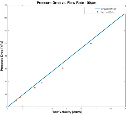
FIGURE 2-4:COMPARISON BETWEEN THE MODEL AND EMPIRICAL RESULTS FOR THE PRESSURE DROP ACROSS THE LENGTH OF A SINGLE CHANNEL IN A FIVE CELL RED STACK WITH NOMINAL INTERMEMBRANE WIDTHS OF 100M [35] ... 46

FIGURE 2-5:COMPARISON BETWEEN THE MODEL AND THE EMPIRICAL RESULTS FOR THE TOTAL OHMIC AREA RESISTANCE PER CELL IN A TWO CELL RED STACK WITH PILLAR PROFILED AEMS

[39] ... 47 FIGURE 2-6:COMPARISON BETWEEN THE PREDICTED AND MEASURED GROSS POWER DENSITY FOR A

RED STACK WITH PILLAR PROFILED AEMS [39] ... 48

FIGURE 2-7:COMPARISON BETWEEN THE MODEL AND EMPIRICAL RESULTS FOR THE PRESSURE DROP ACROSS THE LENGTH OF A SINGLE PROFILED CHANNEL IN A TWO CELL RED STACK WITH NOMINAL INTERMEMBRANE WIDTHS OF 100M [39] ... 49

FIGURE 3-1:NET POWER PER RED STACK VOLUME AS A FUNCTION OF TWO RED STACK DESIGN PARAMETERS USING PROFILED MEMBRANE CHARACTERISTICS FROM GÜLER ET AL.[39] ... 54 FIGURE 3-2:DESIGN OPTIMIZATION CURVES FOR A RED STACK WITH PROFILED MEMBRANES

WHICH SHOW THE MAXIMUM POWER DENSITY ACHIEVABLE WHILE HOLDING ALL OTHER

VARIABLES CONSTANT AT PREVIOUSLY DETERMINED OPTIMUMS ... 56

FIGURE 3-3:OPTIMIZATION CURVES DEPICTING THE THERMODYNAMIC EFFICIENCY OF A RED STACK WHILE HOLDING ALL OTHER VARIABLES AT THEIR DESIGNATED OPTIMUM IN ORDER TO ACHIEVE THE HIGHEST VOLUMETRIC POWER DENSITY ... 57

FIGURE 3-4:DESIGN OPTIMZATION CURVES (USING 504 DATA POINTS) FOR A 50 CELL RED STACK USING PILLARED PROFILED MEMBREANES WITH A FIXED FLOW LENGTH OF 10 CM AND HEIGHT OF 20 CM WITH VARIED HIGH AND LOW CONCENTRATION CHANNEL WIDTHS AND FLOW RATES. THE OPTIMUM CHANNEL WIDTH AND FLOW VELOCITY WERE FOUND TO BE 53.2M AND 81.5

M AND 3.91 CM/S AND 7.54 CM/S FOR THE LOW AND HIGH CONCENTRATION CHANNELS RESPECTIVELY. ... 59

(12)

12

FIGURE 3-5:NET POWER PRODUCTION FOR A 100 CELL RED STACK OPERATING AROUND 4C OVER A DEPTH OF 30M AS A FUNCTION OF DRAW AND FEED SOLUTION CONCENTRATION IN

PRACTICAL SALINITY UNITS ... 61

FIGURE 3-6:TORNADO PLOT OF RED NET POWER COMPARED TO BASELINE VALUES ... 63

FIGURE 3-7:VOLUMETRIC AND SPECIFIC POWER DENSITY COMPARISON BETWEEN VARIOUS

ENVIRONMENTAL ELECTRICAL ENERGY HARVESTING DEVICES THAT COULD BE UTILIZED BY A MOVING SYSTEM [65]–[67]. ... 65

FIGURE 3-8:COMPARISON BETWEEN LITHIUM ION BATTERIES AND RED ON A VOLUMETRIC (TOP) AND SPECIFIC (BOTTOM) POWER DENSITY BASIS.THE POINT OF INTERSECTION

(APPROXIMATELY 10.4 DAYS FOR THE VOLUMETRIC COMPARISON AND 3 DAYS FOR THE MASS BASED) IS THE DURATION OF TIME AT WHICH A RED CELL WOULD BE ABLE TO PROVIDE THE SAME ENERGY TO A SYSTEM AS A COMPARABLE VOLUME OR MASS OF LITHIUM ION BATTERIES.

... 67 FIGURE B-1:PRESSURE DROP VERSUS FLOW RATE PER UNIT HEIGHT (MM2/S) FROM VERMAAS ET

AL.[35] FOR A SPACER-FILLED RED STACK WITH AN INTERMEMBRANE WIDTH OF 60M.THE CORRESPONDING SLOPE OF THE TRENDLINE WAS USED AS A CORRECTION FACTOR FOR THE PUMPING LOSSES, AS THE PRESSURE DROP IS LINEAR WITH THE FLOW VELOCITY. ... 74

FIGURE B-2:PRESSURE DROP VERSUS FLOW RATE PER UNIT HEIGHT (MM2/S) FROM VERMAAS ET AL.[35] FOR A RED STACK WITH A NOMINAL INTERMEMBRANE WIDTH OF 100M ... 75

FIGURE B-5:GRAPH OF THE FOUR SLOPES FROM THE TRENDLINES IN FIGURES A-1 TO A-4 VERSUS THE INTERMEMBRANE WIDTH OF THE STACK ... 76

FIGURE B-6:GRAPH OF THE PUMPING LOSS CONSTANTS FOR THE DILUTE CHANNEL CALCULATED FROM THE CONSTANTS IN FIGURE A-5 AND MODIFIED SO AS TO BE USED WITH THE DARCY -WEISBACH EQUATION.THE RESULTING CURVE WAS USED TO PREDICT THE CORRECTION FACTOR FOR THE PUMPING LOSS OF VARIOUS RED STACKS AT INTERMEMBRANE DISTANCES BETWEEN 60 AND 485M. ... 77

(13)

13

FIGURE B-7:GRAPH OF THE PUMPING LOSS CONSTANT FOR THE CONCENTRATED CHANNEL

CALCULATED FROM THE CONSTANT IN FIGURE A-5 AND MODIFIED SO AS TO BE USED WITH THE

DARCY-WEISBACH EQUATION.THE RESULTING CURVE WAS USED TO PREDICT THE

CORRECTION FACTOR FOR THE PUMPING LOSS OF VARIOUS RED STACKS AT INTERMEMBRANE DISTANCES BETWEEN 60 AND 485M. ... 77

FIGURE B-8:PRESSURE DROP VERSUS FLOW RATE PER UNIT HEIGHT (MM2/S) FROM GÜLER ET AL.

[39] FOR A RED STACK WITH PROFILED MEMBRANES AT AN INTERMEMBRANE DISTANCE OF

100M.THE CORRESPONDING SLOPE OF THE TRENDLINE WAS USED TO DERIVE A CORRECTION FACTOR FOR DARCY-WEISBACH EQUATION FOR PROFILED CHANNELS. ... 78

FIGURE C-1:COMPARISON BETWEEN THE MODEL AND EMPIRICAL RESULTS FOR THE TOTAL RESISTANCE PER CELL (TOP LEFT), GROSS POWER PER MEMBRANE AREA (TOP RIGHT),

PRESSURE DROP ALONG A CHANNEL (BOTTOM LEFT), AND NET POWER PER MEMBRANE AREA

(BOTTOM RIGHT) PRODUCED BY A FIVE CELL RED STACK WITH NOMINAL INTERMEMBRANE WIDTHS OF 60M (61M MEASURED)[35] ... 79

(BOTTOM RIGHT) PRODUCED BY A FIVE CELL RED STACK WITH NOMINAL INTERMEMBRANE WIDTHS OF 485M (455M MEASURED) [35] ... 81

(14)

14

FIGURE C-5:COMPARISON BETWEEN THE MODEL AND EMPIRICAL RESULTS FOR THE GROSS POWER PER MEMBRANE AREA, PUMPING POWER PER MEMBRANE AREA, AND NET POWER PER PUMPING AREA FOR A 50 CELL RED STACK WITH NOMINAL SPACING OF 200M [64] ... 81

FIGURE C-6:COMPARISON BETWEEN THE MODEL AND EMPIRICAL RESULTS FOR THE NET POWER PER MEMBRANE AREA OF A PROFILED CHANNEL IN A TWO CELL RED STACK WITH NOMINAL INTERMEMBRANE WIDTHS OF 100M [39] ... 82

FIGURE D-1:PUMPING POWER LOSSES FOR RED STACKS OF VARIOUS INTERMEMBRANE WIDTHS AS A FUNCTION OF TEMPERATURE.THE STACKS’ HEIGHT AND LENGTH ARE 10 CM RESPECTIVELY AND THE FLOW RATE SIMULATED IS 1 CM/S.THIS GRAPH ILLUSTRATES THE LARGE ROLE THAT TEMPERATURE HAS IN INCREASING THE PUMPING LOSSES FOR SMALL CHANNEL STACKS DUE TO THE SENSITIVITY OF WATER’S DYNAMIC VISCOSITY TO LOW TEMPERATURES. ... 83

(15)

15

List of Tables

TABLE 2.1:ROOT MEAN SQUARE DEVIATIONS OF THE MODEL COMPARED TO EXPERIMENTAL

DATA ... 50

TABLE 3.1:BASELINE VALUES FOR TORNADO PLOT ... 62

(16)

16

(17)

17

Chapter 1 Introduction and Background

One form of renewable energy that has received increased interest due to its enormous

untapped potential is salinity gradient power (SGP), which is the controlled Gibbs free energy of

mixing between two water sources of differing salt concentrations. This mixing occurs naturally at river estuaries, beneath icebergs, and along the ocean’s surface following heavy rainfall, but

the energy is often dissipated as entropy. This represents wasted chemical energy, which is

released during this mixing process. The energy released is equivalent to the kinetic energy of an equal mass of water falling from a 270m waterfall, with an energy density of 0.81 kWh/m3_of water [1]. It has been estimated that the global theoretical potential of SGP is 1.4-2.6 TW, of

which 60% is thought to be harvestable [2], [3], [4]. Consequently, SGP holds significant

promise as an alternative energy source.

The concept of SGP was first proposed by Pattle in 1954 [5] and has since expanded into

a variety of methods by which to harness this chemical potential of mixing. The three primary

means of producing salinity gradient power that have received the most attention are capacitive

mixing, pressure-retarded osmosis (PRO), and reverse electrodialysis (RED) [6]. However, while

recent research has focused primarily on the use of SGP for large-scale commercial power plants

[6]–[10], little research has concentrated on the applications of SGP with regards to energy

harvesting for small systems, such as unmanned underwater vehicles (UUV) or remote sensing

devices. For such applications, specific and volumetric power density take precedence over those

(18)

18

metric of power per cost) or the levelized cost of electricity. This thesis explores the feasibility of

using RED as an environmental energy harvester for remote sensing devices and unmanned

underwater vehicles, with a specific focus on the Arctic Ocean.

1.1 Salinity Gradient Power

1.1.1 Gibbs Free Energy of Mixing

During the uncontrolled mixing of two solutions of dissimilar concentrations the Gibbs free energy

of mixing, ∆𝑮_𝒎𝒊𝒙, is released to the environment. This released chemical energy represents the maximum potential energy that can be harvested through an engineering process. The Gibbs free

energy released per mole during the mixture of two solutions is given below:

−∆𝐺_𝑚𝑖𝑥 = 𝑅_𝑔𝑎𝑠𝑇 ( [∑ 𝑥_𝑖ln(𝛾_𝑖𝑥_𝑖)] 𝑀− 𝜙𝐴[∑ 𝑥𝑖ln(𝛾𝑖𝑥𝑖)]𝐴 −𝜙_𝐵[∑ 𝑥_𝑖ln(𝛾_𝑖𝑥_𝑖)] 𝐵 )

where 𝑅𝑔𝑎𝑠 is the ideal gas constant, 𝑇 is the temperature of the mixture, 𝑥𝑖 is the mole fraction of component 𝑖, 𝛾_𝑖 is the activity coefficient of component 𝑖 which accounts for the non-ideal behavior of the solution, and 𝜙 is the ratio of moles in solution A or B to that of the final solution

M [1].

In the specific case of fresh and salt water mixing, both of which have relatively low

concentrations, the mole fraction 𝑥_𝑤 and activity coefficient 𝑦_𝑤 of water are close to unity, causing their respective terms to drop out. Additionally, the concentrations of all other solutes are

neglected, while the contributions of NaCl to the total volume and number of moles is minor. Then, (0.1)

(19)

19

by assuming that the total volume of the mixing solutions is constant, one can approximate the

mole fraction with the molar salt concentration as seen in equation ((1.2):

−∆𝐺𝑚𝑖𝑥,𝑉𝐴 𝜐𝑅_𝑔𝑎𝑠𝑇 ≈ 𝑐_𝑀 𝜙_𝐴ln 𝛾𝑠,𝑀𝑐𝑀− 𝑐𝐴ln 𝛾𝑠,𝐴𝑐𝐴− (1 − 𝜙_𝐴) 𝜙_𝐴 𝑐𝐵ln 𝛾𝑠,𝐵𝑐𝐵

where ∆𝐺_{𝑚𝑖𝑥,𝑉}_𝐴 is the Gibbs free energy per volume of solution A, υ is the number of ions into which each electrolyte molecule will dissociate into (2 for 𝑁𝑎𝐶𝑙), and c is the molar

concentration of 𝑁𝑎𝐶𝑙 in solutions A, B, or M, and the subscript s denotes the activity coefficient specifically for salt [1].

Finally, one can assume ideal behavior such that the activity coefficients are negligible.

Equation 1.2 can then be simplified to equation (1.3) [1]:

−∆𝐺𝑚𝑖𝑥,𝑉𝐴 𝜐𝑅_𝑔𝑎𝑠𝑇 ≈ 𝑐_𝑀 𝜙_𝐴ln 𝑐𝑀 − 𝑐𝐴ln 𝑐𝐴 − (1 − 𝜙𝐴) 𝜙_𝐴 𝑐𝐵ln 𝑐𝐵

1.1.2. Capacitive Mixing (CapMix)

Capacitive mixing was first proposed in 2009 [11] as an electrochemical means of directly

producing electrical power, with RED previously being the only means of direct conversion. A

capacitive mixing cell includes two electrodes, which are initially immersed in a high

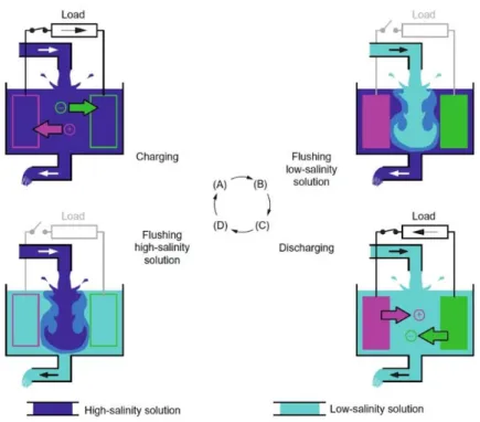
concentration salt solution and are connected via an electrical circuit. As shown in Figure 0-1,

the process consists of four distinct parts:

(0.3) (0.2)

(20)

20

Figure 0-1: Four-step overview of the capacitive mixing cycle highlighting the system’s conversion of chemical to electric potential

A. Current is applied to the electrodes, causing the electrodes to become charged. This induces cations (Na+_{) and anions (Cl}−_{) to migrate to and form a thin layer on the} negatively and positively charged electrodes respectively, in order to balance the local

charges.

B. The circuit is disconnected and the high concentration solution is flushed with a low

concentration solution. Replacing the high concentration solution with one of a lower

ionic strength causes the thickness of the charged layer surrounding the electrodes to

increase. This increases the electrical potential of the cell.

C. The circuit is reconnected. The lower concentration of the dilute solution induces

some of the ions that have collected on the electrodes to discharge in order to approach

(21)

21

charge collected on the electrodes flows through the circuit producing a current in the

direction opposite to that applied in part A.

D. The circuit is opened and the low concentration solution is replaced with high

concentration solution. Since the discharge of electrons in part C occurs at a higher

electrical potential than when the current is applied in part A, net work is produced [7],

[13].

While novel, capacitive mixing is still in the very early phases of its development and has

not yet been put to use in real world applications. Its highest reported experimental power density of 0.2 W/m2_{is an order of magnitude smaller than those obtained for both PRO and} RED [13]. Consequently, while it may hold future potential, capacitive mixing was not deemed a

currently viable means of powering UUVs and remote sensing systems.

1.1.3 Pressure Retarded Osmosis (PRO)

The concept of PRO, first articulated by Sidney Loeb in 1975 [14], involves the production of

mechanical power through the use of a water selective membrane to produce a pressure gradient.

Figure 0-2 illustrates how PRO works. Two volumes of high concentration and low

concentration fluids are separated by a semipermeable membrane that prevents the flow of ions

from one solution to the other. Consequently, an osmotic pressure gradient is produced across the

membrane, which drives water from the low concentration solution to the more concentrated

solution. This increase in volume in the concentrated solution compartment can be directly

(22)

22

Figure 0-2: (A) Diagram illustrating the operation of PRO with water flowing across the semipermeable membrane from the low concentration solution to the high concentration solution

and being harnessed to produce power. (B) Graph of the osmotic pressure ∆𝜋 versus the displaced water, 𝑉_𝑝 and the resultant useful work that can be achieved from a PRO system at a

fixed applied pressure ∆𝑝 [6].

The useful work that can be harnessed from PRO is found by integrating the applied hydraulic pressure, ∆𝑝, which in practical applications is constant, by the displaced volume of water, 𝑉_𝑝, as given in equation (1.4) [6]:

𝑊 = ∫ ∆𝑝𝑑𝑉_𝑝

This useful work is depicted in Figure 0-2 (B) as the blue shaded region and is highly dependent

on the selectivity and structural strength of the semipermeable membrane used [15]. A study by

Yin Yip and Elimelech estimated the theoretical power density per membrane area and

thermodynamic efficiency of PRO given the current technological state of PRO membranes to be between 2.4-3.7 W/m2_{and 44-54% respectively, depending on the concentration of the two} mixing solutions [16].

PRO has seen a large growth in academic and commercial interest in the last ten years.

Recent research has focused largely on improving membrane selectivity and structural strength,

in addition to the application of PRO to areas with highly concentrated salt water, i.e. the Dead (0.4)

(23)

23

Sea, and its use with reverse osmosis plants [15]. The power company Statkraft opened the first

PRO power plant in Tofte, Norway in 2009, as can be seen in Figure 0-3, although plans for the plant’s expansion were discontinued in 2014, due to the plant’s low efficiency and uneconomical

returns on investment [6].

Figure 0-3: Statkraft PRO Power plant in Tofte, Norway [17]

However, for the purpose of applying SGP to small unmanned vehicles or remote sensing

devices, PRO was deemed a poor candidate. This decision was made because PRO would require

a microturbine to provide electrical power, which generally has low efficiency. While PRO could

be used as a direct propulsion system for UUVs, such a use would require a complete redesign of

current long-range UUV platforms, which are largely powered electrically by lithium ion

(24)

24

1.1.4 Reverse Electrodialysis (RED)

RED was first proposed and demonstrated by Richard Pattle between 1954 and 1955 [5], [19] and saw further development with George Murphy’s use of RED to power an electrodialysis

(ED) desalination process, a process he named “osmionic demineralization” [20], [21]. Lacey further developed Murphy’s concept in 1960 [22], but it was not until an impetus from the first

and second oil crisis in 1973 and 1979 that interest in RED was truly heightened [23]. In 1976

Weinstein and Leitz improved the previous experimental power density achieved by Pattle by a factor of three to 170 mW/𝑚2_{[24] and in 1980 Lacey published a paper modeling RED power} production with varying parameters and the consequent costs associated with a commercial RED

power plant [25]. In 2001Veleriy Knyazhev reportedly conducted the first RED test in the field,

using river and seawater [26]. In the following years extensive research has been carried out by

the Wetsus Institute in the Netherlands on the topic, including five doctoral theses dedicated to the various aspects of RED [27]–[31]. Additionally, Bruce Logan from Pennsylvania State, Menachem Ehimelech from Yale, and Ngai Yin Yip from Columbia have published several

articles analyzing the broader thermodynamic potential and constraints of RED and comparing it

(25)

25

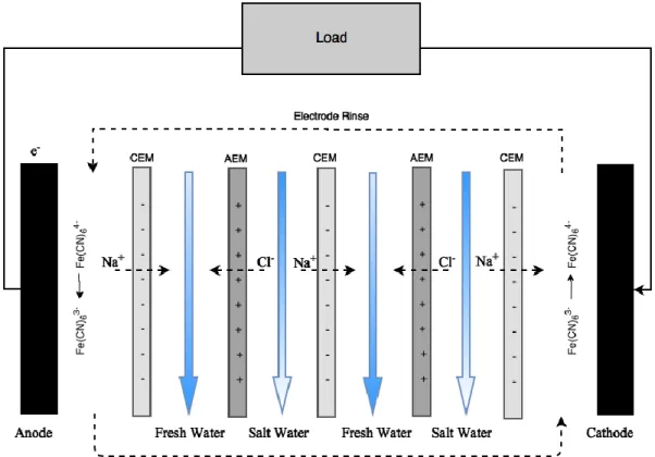
Figure 0-4: Schematic of an RED cell where a 𝐾4𝐹𝑒(𝐶𝑁)6/ 𝐾3𝐹𝑒(𝐶𝑁)6 solution is used as the electrolyte with inert electrodes

Figure 0-4 illustrates how an RED stack operates. High and low concentration water flow

through alternating channels separated by a series of cation exchange membranes (CEM) and

anion exchange membranes (AEM), which only allow the permeation of cations or anions

respectively. As the water flows through the varying channels, ions from the high concentration

solution will travel across the CEMs and AEMs due to osmosis to the less concentrated solution,

creating an ion flux across the stack. In order to balance the charge at the respective electrodes, a

redox reaction occurs and an electrical current is generated.

Analytically, the power generated by an RED stack is dependent on the total voltage across

(26)

26 𝑉_{𝑠𝑡𝑎𝑐𝑘} = 𝑛_{𝑐𝑒𝑙𝑙}(𝛼𝐴𝐸𝑀 𝑧₋ + 𝛼_𝐶𝐸𝑀 𝑧₊ ) 𝑅_𝑔𝑎𝑠𝑇 𝐹 ln ( 𝐶_𝐻 𝐶_𝐿)

For equation (1.5) 𝑛_{𝑐𝑒𝑙𝑙} is the number of cells, 𝛼 is the permselectivity of the anion and cation exchange membranes, 𝑧 is the ion valence (1 for 𝑁𝑎+_{and 𝐶𝑙}−_{), 𝐹 is Faraday’s constant, and C is} the concentration in g NaCl per kg of solution of the high (H) and low (L) concentration solutions respectively. Assuming that maximum power is achieved by matching the impedance, the power

applied to the load is then:

𝑃_{𝑠𝑡𝑎𝑐𝑘} = 𝑉𝑠𝑡𝑎𝑐𝑘 2 4𝑅_{𝑠𝑡𝑎𝑐𝑘} where 𝑅𝑠𝑡𝑎𝑐𝑘 is the stack’s resistance.

Accounting for the pumping power the net power becomes

𝑃_𝑛𝑒𝑡 = 𝑃_{𝑠𝑡𝑎𝑐𝑘}− 𝑃_{𝑝𝑢𝑚𝑝}

The highest reported net power density per membrane area produced using fresh and

seawater is 1.2 W/m2_{and was achieved by Vermaas in 2011[35], while the highest overall power} density is 6.7 W/m2_{, which Daniilidis et al. achieved in 2014 using fresh water and concentrated} brine [36]. The characteristics of CEMs and AEMs have been the focus of much recent research

with some studies exploring the effects of lowering membrane resistances through creating thinner

stronger membranes [37]. Additionally, research has explored the possibility of using counter flow

or cross flow (where the flows are 90 to one another), which have been shown to increase power

output and efficiency, although once again stronger membranes would need to be developed to

deal with the potential bending induced by dissimilar pressures along the channels [33]. New

profiled membranes which omit the need for spacers, and consequently omit the spacer shadow

effect (blockage of the membrane by the spacer), have also been shown to reduce the pressure drop (0.6)

(0.7) (0.5)

(27)

27

along the channel length, thus reducing pumping losses and greatly improving the overall net

power [38]–[41]. The need to improve the monovalent permselectivity of CEMs and AEM has

been identified as one area that could lead to significant improvements in the performance of RED,

as the flux of even a few multivalent ions greatly reduces the power generated by 29% to 50%

[42]. While RED research has focused heavily on membrane technology, the use of segmented

electrodes along the length of the RED channel to better match the load and increase the maximum

power output has also been proposed [43], [44].

Currently, two RED test power plants are in operation, one on the Afsluitdijk dam in the

Netherlands and the other in Marsala, Italy. The RED plant in the Netherlands, pictured in Figure

0-5 was opened in 2014 with the aim of eventually producing between 0.5-2MW and is operated

by REDstack, a spinoff from the Wetsus Institute in collaboration with Fujifilm. The plant utilized

fresh water flowing from the Rhine and seawater from the Waddenzee to produce power,

discharging the brine back into the sea to prevent the dam from flooding [45]. In contrast, the

Reverse Electrodialysis Alternative Power (REAPower) Project in Sicily, sponsored by the

European Union and REDstack, uses concentrated brine from a nearby salt works and brackish

water. Research at the plant aims to achieve 1kW, with recent efforts achieving 700W using

(28)

28

Figure 0-5: REDstack power plant situated on the Afsluitdijk dam between the Ijsselmeer and the Waddenzee [46]

In assessing RED’s potential for use with small-scale mobile platforms, it is worth noting

that while recent studies comparing RED and PRO have predicted a higher theoretical power

density for PRO [16], RED has several unique advantages. These advantages include RED’s

ability to directly produce electrical power and a design that allows for more ready integration

into current UUV and sensor systems, which rely on battery power. Consequently, RED was

selected as the SGP technology best suited for potential future application into UUV and remote

sensing systems.

1.2. RED Applications

1.2.1 Geographic Areas of Interest

As illustrated in equation (1.5) and equation (1.6), the power output from RED is proportional to

the square of the logarithmic ratio of the high to low concentration. Consequently, the areas

where RED can be applied are restricted to a limited number of key geographic regions. In

(29)

29

River Delta, the Rhine River, the St. Lawrence River, etc., the polar regions also contain a

significant salinity gradient during the summer months.

Figure 0-6: Global salinity ratio of the highest to lowest concentrations between 0 and 30m for the month of August with data compiled from GDEM [47]

As shown in Figure 0-6, in addition to the mouths of large rivers, such as the Ganges and

Amazon, a substantial ratio of salt to fresh water can be found within the top 30 meters below

sea surface in the Arctic region. Additionally, it should be noted that the data in Figure 0-6 does

not accurately capture much of the local concentration gradient found in the Artic.

1.2.2 Application to the Arctic

The Arctic Circle has become a region of increased attention to both the scientific and defense

communities as of late. As the effects of global warming increasingly make their presence felt on

the world, the need to collect climate data for sustained periods in the Arctic region has grown in

importance. Additionally, from a security perspective, the melting of the icecaps will increase demand for access to the region’s new trade routes and abundant natural resources [48].

(30)

30

However, the region’s harsh weather and currently significant ice-coverage, as depicted in Figure

0-7, continues to present a challenging operational environment. The predominant power sources

in the region are diesel generators or batteries, both of which rely on costly periodic resupplies of

fuel or, in the case of primary batteries, replacement.

Figure 0-7: Map of the Arctic Circle showing the minimum extent of sea ice both in 2012 (red line) and on average for the past 30 years [48]

As previously depicted in Figure 0-6, substantial salinity gradients develop in the Arctic

during the summer months. Increased periods of exposure to sunlight cause small ponds of fresh

water to form on the surface of the ice. Since the fresh water is denser than the ice, some of this

water will percolate through the ice, forming small fresh water ponds on top of the denser

(31)

31

Figure 0-8: Illustration of how melt ponds on the surface percolate through the ice to create a boundary layer of fresh water [49]

These ponds lead to thin boundary layers directly below the ice with extremely sharp salinity

gradients ideal for SGP. Protected from wind, these freshwater “ponds” persist for a sustained

period of time, as shown inFigure 0-9, until a storm or other phenomena induces mixing.

Through SGP, these sharp salinity gradients represent readily accessible energy reservoirs in an

otherwise bleak and austere environment, barren of otherwise readily accessible power sources.

Figure 0-9: Salinity concentration directly under an ice floe between the months of July and August [50]

Salinity (g NaCl/ kg 𝐇

𝟐

𝐎

)

D

ept

h

(m

)

0

1.5 Time (day)

10 July 10 Aug

(32)

32

1.2.3 Applications to Small Mobile Platforms

As previously mentioned, RED holds potential for application to small UUV platforms or remote

sensing devices facing certain environmental constraints. According to the U.S. Navy, lithium ion

batteries are currently the power system of choice for small scale UUVs, due to their ability to be

easily downscaled for platforms with volumetric limitations (in contrast to fuel cells or hybrid

diesel/ rechargeable battery systems) and their high energy density in comparison to other battery

systems [51]. However, lithium ion batteries are presently not sufficient to power a UUV for the

breadth of the polar regions, where the smallest expanse covered by Arctic sea ice in recorded

history is 1.3 million square miles [48]. While solar power has often been implemented to extend

battery ranges in the past, photovoltaic power is not a viable option for travel under the ice or at

significant underwater depths, with power outputs at depths of 8m falling to levels as low as 1.5%

of that at the surface [52], [53]. Consequently, RED poses a potential means of energy harvesting

to supplement traditional energy storage systems such as lithium ion batteries.

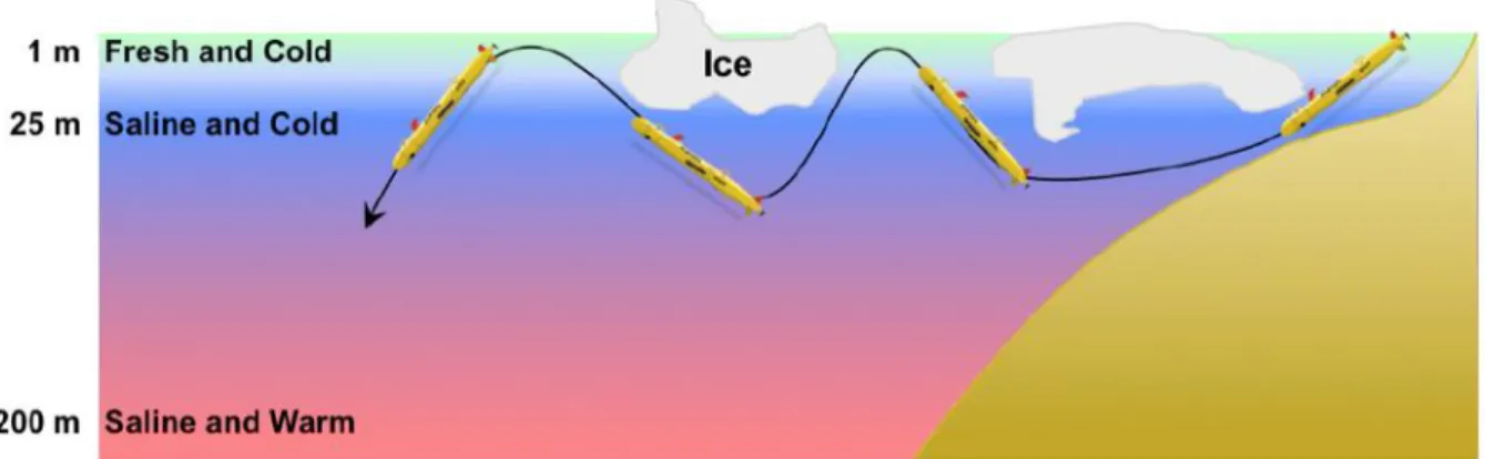
One potential means of travel for such a system would be a sinusoidal dive pattern, as

depicted in Error! Reference source not found., collecting fresh water at the surface and then

travelling downward to collect salt water at around 25-30m underwater. A UUV could also

consistently float under one iceberg where the salinity gradient is significantly shallow, as in Figure

(33)

33

Figure 0-10: Proposed dive profile of a RED powered UUV

In addition to potentially supplementing existing UUV power systems, RED also holds

potential for use with remote sensing devices. By tethering a remote sensing system under an

iceberg, a sensor would be able to float around a region while harvesting power through RED,

requiring only a means of vertical transport between the regions of differing concentration. RED

could also be employed using the surface melt pond, depicted in Figure 0-8, as a fresh water

reservoir and seawater for a high concentration source in order to produce power for a small

sensing device on the surface. An application to river delta regions, where tidal currents allow for

a predictable cycle of fresh and salt water, is the concept of tethering a buoy to the sea floor, which

would collect fresh and salt water with the tides in order to produce power. Such a device could

discretely collect data without any moving parts for an extended period of time, without having to

(34)

34

(35)

35

Chapter 2 Computational Modeling

In order to form an analytical assessment of RED and its potential as a power source for

remotely operated vehicles and sensing devices, a computational code modeling the underlying

phenomena of RED was created from a combination of fundamental theoretical and empirical

equations. The code was modeled on a similar approach taken by Vermaas [54], with additional

adjustments made to focus on various aspects of RED pertaining to potential use by naval

vessels. The model consisted of a parameter sweep of the key variables affecting a RED stack, i.e. the height h and length l of the active membrane area, the width between the membranes w,

and flow velocity v, which are depicted in Figure 0-1. This parameter sweep then found the

optimal dimensions and flow rates for a theoretical RED stack in order to maximize the net

power density of the system at the optimal naturally occurring concentrations.

While past studies have either limited their models to specific RED stack designs with

ample empirical validation or focused on broad assessments with limited experimental

validation, this model assesses a wide range of possible RED stack parameters, while generating

results largely consistent with a diverse range of past experimental studies. Unlike past studies, it

focuses on optimizing the net volumetric power density, rather than the net power density per

membrane area, as the volumetric power density is of greater concern for utilization in small

mobile platforms. Additionally, the model accounts for the buoyant energy losses incurred by

having to transport volumes of water of dissimilar densities from a specified depth to the surface

(36)

36

commercial power. The model also incorporates the flexibility to estimate the net power

densities for both spacer-filled channels and those with profiled membranes, while providing

empirical validation for both designs. Finally, it considers the viscosity and density of water as

variables of the input temperature, pressure, and water concentrations, allowing for more

accurate power predictions in a diverse set of environmental conditions. These features allow for an initially broad optimization of RED’s design parameters followed by a more precise analysis

of its potential in the Artic versus other potential environmental energy harvesters.

2.1 Governing Equations and Assumptions

2.1.1 Key Assumptions

In constructing the computational model, several key assumptions were made in order to

simplify the modeling. These assumptions include:

1. Matched impedance between the stack and load (𝑅_{𝑙𝑜𝑎𝑑} = 𝑅_{𝑠𝑡𝑎𝑐𝑘})

2. Flow between the channels can be modeled as laminar flow between two infinite parallel

plates

3. A linear salinity gradient from the surface to the depth of 30m

4. The effects of parasitic currents are negligible.

5. The effects of membrane fouling are negligible.

For electrical power systems, maximum power is often achieved by matching the

impedance of the stack and load. While Weiner et al. showed that this is not the case, due to the

drop in voltage along the RED channel, this assumption nevertheless provides a conservative

estimate as to the maximum achievable power [10]. The assumption that the flow can be

(37)

37

rates and small hydraulic diameter of the channels led to low Reynolds numbers for the

parameter space of interest. This was verified by calculating the percentage of computational

data points for which the flow was laminar, with the results coming close to unity. Additionally,

the channel height in a RED stack is often several orders of magnitude greater than the channel

width, thus justifying the approach of modeling the membranes as infinite parallel plates. The

third assumption was necessary, primarily to effectively model the buoyant force losses incurred

by transporting volumes of water with dissimilar densities. Regarding the effect of parasitic

currents, Veerman et al. showed that through careful stack design these losses in efficiency could

be reduced from 25% to 5%, mitigating these losses even for large stacks [55]. While the effects of membrane fouling have been shown to decrease net power density by as much as 40% within

one day of testing [56], methods such as reversing the fresh and concentrated water channels and

the development of membranes with improved monovalent selection can reduce these losses

[57], [58].

2.1.2 Fundamental Equations

Stemming from the Nernst equation, equation (1.5) gives the theoretical voltage that is produced

from the ion flux across the stack (refer to Appendix A for a table of the key variables and their

units). 𝑉𝑠𝑡𝑎𝑐𝑘 = 𝑛𝑐𝑒𝑙𝑙( 𝛼_𝐴𝐸𝑀 𝑧− + 𝛼_𝐶𝐸𝑀 𝑧+ ) 𝑅_𝑔𝑎𝑠𝑇 𝐹 ln ( 𝐶_𝐻 𝐶𝐿) The power applied to the load is then

𝑃_{𝑠𝑡𝑎𝑐𝑘} = 𝐼_{𝑠𝑡𝑎𝑐𝑘}2 𝑅_{𝑙𝑜𝑎𝑑} 𝑃_{𝑠𝑡𝑎𝑐𝑘} = 𝑉𝑠𝑡𝑎𝑐𝑘2𝑅𝑙𝑜𝑎𝑑 (𝑅𝑠𝑡𝑎𝑐𝑘+𝑅𝑙𝑜𝑎𝑑)2 (0.1a) (2.1b) (1.5)

(38)

38 𝑃𝑠𝑡𝑎𝑐𝑘 = 𝑉𝑠𝑡𝑎𝑐𝑘

2_𝑅 𝑙𝑜𝑎𝑑

[𝑛𝑐𝑒𝑙𝑙×(𝑅𝑜ℎ𝑚𝑖𝑐+𝑅𝐵𝑙+𝑅∆𝐶)+𝑅𝑙𝑜𝑎𝑑]2

where 𝐼_{𝑠𝑡𝑎𝑐𝑘} is the current and R is the resistance due to the load, ohmic losses, boundary layer losses, and losses along the channel’s length due to a decrease in the difference of concentration

between the flows [54]. These resistances are dependent on various membrane and spacer

properties, solution concentrations, and the specific dimensions of the stack itself as pictured in

Figure 0-1.

Figure 0-1: Schematic of the membrane orientation in a RED stack highlighting the key parameters which impact the stack’s performance and were the subsequent focus of the

computational modeling

The ohmic area resistance 𝑟_{𝑜ℎ𝑚𝑖𝑐} is due to electrical resistance from the membranes and the channels themselves as given below.

𝑟_{𝑜ℎ𝑚𝑖𝑐} = 1 1 − 𝛽∙ (𝑟𝐶𝐸𝑀 + 𝑟𝐴𝐸𝑀) + 1 𝜀2_{∙ 𝑘}0 𝐶₀ ∙ (𝑤𝐻 𝐶_𝐻 + 𝑤_𝐿 𝐶_𝐿) (2.1c) (0.2)

(39)

39

𝛽 is the masking factor due to the spacer shadow effect on the membrane, r is the area resistance of the CEM and AEM respectively, w is the intermembrane width of the high and low

concentration channels, 𝜀 is the porosity of the channel between the membranes, 𝑘₀ is the electrical conductivity of seawater at standard temperature and pressure, and 𝐶₀ is the reference concentration of seawater (35 g NaCl per kg).

The boundary layer resistance due to concentration polarization across the membrane is

given empirically by Vermaas et al. for both spacer-filled channels and profiled membranes [54].

𝑟_{𝐵𝐿,𝑠𝑝𝑎𝑐𝑒𝑟𝑠} = (0.62 ∙ 𝑡_𝑟𝑒𝑠∙𝑤

𝐿 + 0.05 ) 𝑟_{𝐵𝐿,𝑝𝑟𝑜𝑓𝑖𝑙𝑒𝑑} = (0.96 ∙ 𝑡_𝑟𝑒𝑠 ∙𝑤

𝐿 + 0.35 )

with 𝑡_𝑟𝑒𝑠 as the residence time, which is the quotient of flow velocity v and the membrane length

L. The resistance due to a decrease in concentration along the membrane length L can be

approximated by (2.4a): 𝑟_∆𝐶 = (𝛼𝐴𝐸𝑀+ 𝛼𝐶𝐸𝑀 2 ) 𝑅_𝑔𝑎𝑠∙ 𝑇 𝑧 ∙ 𝐹 ∙ 𝑗 ln( 𝐴𝐿 𝐴_𝐻) Where 𝐴_𝐿 = 1 + 𝑗 ∙ 𝑡𝑟𝑒𝑠 𝐹 ∙ 𝜀 ∙ 𝑤_𝐿∙ 𝐶𝐿 𝑀_𝑆 𝐴_𝐻 = 1 − 𝑗 ∙ 𝑡𝑟𝑒𝑠 𝐹 ∙ 𝜀 ∙ 𝑤_𝐻∙ 𝐶𝐻 𝑀_𝑆

With M being the molecular weight of NaCl and where 𝑗, the current density is given by: 𝑗 = 𝑉𝑡𝑜𝑡𝑎𝑙 𝑟_{𝑠𝑡𝑎𝑐𝑘}+ 𝑟_{𝑙𝑜𝑎𝑑} (0.3a) (2.3b) (0.4a) (2.4b) (2.4c) (0.5)

(40)

40

The derivation of equations (2.4a)-c) is given by Vermaas et al. [35]. Assuming a matched

impedance equation, (2.1b) then becomes equation (1.5)

The pressure drop ∆𝑝 along one channel was estimated using the Darcy-Weisbach equation for laminar flow between two infinite parallel plates as shown in equation (2.6) [59],

∆𝑝 = 𝑓 𝐿 𝑑𝐻 𝜌𝑣2 2 = 48𝜇𝐿𝑣 𝑑_𝐻2

where 𝑑𝐻 is the hydraulic diameter. In order to better account for the effect of spacers and profiled ridges in accurately predicting the pressure drop, the hydraulic diameters were adjusted

[54]. The hydraulic diameter for spacer filled membranes is given by equation (2.7a) [60], while

that of profiled membranes is given by equation (2.7b) [60], [61]:

𝑑_ℎ = 4𝜀

2/𝑤 + (1 − 𝜀) ∙ 𝑆_𝑣𝑠𝑝 𝑑ℎ =

4𝑏 ∙ 𝑤 2𝑏 + 2𝑤

where 𝑆_𝑣𝑠𝑝 is the ratio of the spacer surface area to its volume and b is the width between the profiled ridges (which was assumed to be proportional 𝑤). Using data from Vermaas et al. [35] for spacer filled channels, a fit equation as a function of intermembrane width was generated in order to calculate a correction factor 𝐾_𝑝 for the pressure drop for intermembrane distances between 60 and 485 μm, which is the parameter space of interest for optimization. This was accomplished by fitting the pressure drops at intermembrane distances of 61, 101, and 209, and 455 μm. As for profiled membranes, a correction factor was calculated using data provided by Güler et al. [39]. Further information regarding these correction factors can be found in Appendix B. The pumping loss for the entire stack is then:

(0.6)

(0.7a)

(41)

41

𝑃_{𝑝𝑢𝑚𝑝} = 2 ∙ 𝑛_{𝑐𝑒𝑙𝑙} ∙ 𝑄 ∙ 𝐾_𝑝∙ ∆𝑝 Where the volumetric flow rate is given by:

𝑄 = 𝜀 ∙ ℎ ∙ 𝑤 ∙ 𝑣

Optimizing 𝑃_𝑛𝑒𝑡 from equation (1.7) as a function of the fluid velocity v, channel width w, channel height h, and channel length L (as depicted in Figure 0-1) given certain constraints, then allows one

to approximate the idealized dimensions in order to achieve maximum net power per volume stack.

In addition to conducting a parameter sweep in order to predict the potential net power of

a RED stack given certain design specifications, estimates unique to the use of RED for a UUV

were also considered. The most prominent of these additional considerations was the power losses

due to overcoming the buoyant force acting on solutions of differing densities. This buoyant force

loss occurs due to the need to transport denser high concentration seawater through less dense

water to the surface and similarly from transporting less dense freshwater to lower depths through

denser seawater.

Assuming a linear salinity profile the energy E required to transport a volume of water V

was estimated using equation (2.10) below, 𝐸

𝑉 = 1

2(𝜌𝑡𝑜𝑝 − 𝜌𝑏𝑜𝑡) ∙ 𝑔 ∙ 𝑦

where 𝜌 is the density of water at the top and bottom of the UUVs dive profile, g is the acceleration due to gravity, and y is the vertical distance traversed by the UUV from the top to the bottom of its

dive cycle. This is then used to calculate the consequent loss in power, 𝑃_{𝑏𝑢𝑜𝑦𝑎𝑛𝑡} in equation (2.11): 𝑃_{𝑏𝑢𝑜𝑦𝑎𝑛𝑡} = 0.75𝑛_{𝑐𝑒𝑙𝑙} ∙𝐸 𝑉∙ 𝑄 (0.8) (0.9) (0.10) (0.11)

(42)

42

Accounting for 𝑃_{𝑏𝑢𝑜𝑦𝑎𝑛𝑡} one can find the actual power available to provide thrust or power for electronic instrumentation for a UUV or sensor system as shown in equation (2.12)

below.

𝑃_{𝑛𝑒𝑡,𝑚𝑜𝑑} = 𝑃_{𝑠𝑡𝑎𝑐𝑘}− 𝑃_{𝑝𝑢𝑚𝑝}− 𝑃_{𝑏𝑢𝑜𝑦𝑎𝑛𝑡}

The thermodynamic properties of water including its density, dynamic and kinematic viscosity

used in the model were obtained via Matlab scripts produced by Sharqawy et al. [62] and Nayar

et al. [63], given inputs of temperature, pressure, and salinity concentration.

2.2 Model Implementation

The computational model was run on MATLAB utilizing a 4D matrix, which contained the four

variables of interest regarding the design and operation of a RED stack. These values were then

used to compute matrices for the stack’s voltage, ohmic resistance, boundary layer resistance,

and resistance due to the concentration drop along the channel with each point within the matrix

corresponding to a unique combination of variables. A Levenberg-Marquardt solver was then

used to solve for the current density j produced by solving equation (2.13)

0 = 𝑗 − 𝑉𝑠𝑡𝑎𝑐𝑘

2𝑛𝑐𝑒𝑙𝑙× (𝑅𝑜ℎ𝑚𝑖𝑐+ 𝑅𝐵𝑙+ 𝑅∆𝐶) + 𝑅𝑒𝑙𝑒𝑐 + 𝑅𝐶𝐸𝑀

and its subsequent Jacobian. Using these values, the gross power generated by the RED stack, 𝑃_{𝑠𝑡𝑎𝑐𝑘}, was computed. Subsequently the pumping losses were calculated and subtracted from the gross power to find the net power, 𝑃_𝑛𝑒𝑡.

The model was initially run varying the intermembrane width w, channel length L, flow

velocity v, and channel height h. Membrane properties for a profiled AEM from Güler et al. [39] (0.12)

(43)

43

were primarily used for both CEM and AEM membrane properties, as these were deemed to be

the state of the art and yielded higher power densities in agreement with the simulation

performed by Vermaas et al. [54] and the experimental testing performed by Güler et al. [39]. Later iterations focused solely on varying the channel widths and flow velocities of the

respective low and high concentration solution channels.

2.3 Model Validation

2.3.1 Validation for Spacer-Filled Channels

In order to validate the model, experimental results from Vermaas et al. [35] and Veerman et al.

were compared to the model for the spacer-filled case, while results from Güler et al. [39] were

used for the profiled membrane case. For both the spacer-filled channels and the profiled

channels, comparisons were made between the area resistances, gross power densities, the

pressure drops, and the net power densities.

Since the study by Vermaas et al. included measurements at intermembrane distances of 61, 101, 209, and 455μm, the spacer-filled model was consequently evaluated at several channel widths, allowing a more complete validation in the wider parameter space. This section limits

comparison to the total resistance, predicted and experimental gross power, and pressure drop for the 101 μm RED stack, as this was the width at which the highest power density was measured [35]. Further comparisons for the total resistances, gross power densities, pressure drops, and net

(44)

44

Figure 0-2: Comparison between the model and empirical results for the area resistance per cell produced by a five cell RED stack with nominal intermembrane widths of 100 m [35]

Figure 0-2 shows that area resistance predicted by the model is consistently higher than

that measured by Vermaas et al. As the resistance curve levels off beginning at a velocity of 1

cm/s, the model consistently differs from the experimental data by approximately 8.5 − cm2. Upon examining the individual components of the total resistance, it is found that the largest

discrepancies occurs for the ohmic resistance and the boundary layer resistance. The error for the

boundary layer equation most likely stems from the natural limitations of the empirical model given by Equation (2.3a), which was derived from a linear fit (R2 _{= 0.72) [54]. The largest} source of differences in ohmic resistance stems from discrepancies in the resistance produced by the spacer, which likely is due to the challenges in accurately modeling the effects of 𝜀 on the channel resistance, with its effect in equation (2.2) merely given as a first approximation [61].

(45)

45

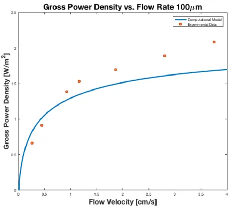
Figure 0-3: Comparison between the model and empirical results for the gross power per membrane area produced by a five cell RED stack with nominal intermembrane widths of 100

m [35]

Figure 0-3 depicts the theoretical prediction of the gross power produced compared to the

experimental values measured by Vermaas et al. It can be seen that the experimental results

appear to lag behind the model by several tenths of a cm/s, while the model predicts power outputs consistently lower than those measured once the curve’s slope begins to level off at

around 1 cm/s. This can be traced back to a comparison in total resistances, as depicted in Figure

0-2, where Vermaas reported resistances consistently lower than those estimated by the model.

While the difference between resistances remains relatively constant, at higher voltages and

(46)

46

becomes more pronounced. However, slightly lower power outputs were expected, since the load

was matched to the stack resistance, which has been shown to be suboptimal [10].

Figure 0-4: Comparison between the model and empirical results for the pressure drop across the length of a single channel in a five cell RED stack with nominal intermembrane widths of 100

m [35]

Figure 0-4 shows close alignment between the pressure drops, as expected given that the

pressure drop was fit to the empirical data. The only variation of note occurs due to that the best

fit line was fixed to the origin, while the trend line for the experimental data was slightly offset.

An additional comparison was also made between results collected by Veerman et al. [64] with a 50 cell stack with intermembrane distances of 200 μm. This was done primarily to check the validity of the model with regards to the pressure drop for other stacks. The maximum

(47)

47

measured pressure drop by Veerman et al. A summary of the root mean square errors between

the various empirical data sets can be found in Table 0.1.

2.3.2 Validation for Profiled Membranes

For the profiled membrane case, the model was compared to a study in which a RED stack with

microstructured AEMs with geometrical structures of pillars, waves, and ridges were compared

to a stack with standard flat AEMs and spacers. The CEMs for all four scenarios, however, were

flat and employed traditional net spacers. Comparisons were made to the pillared case, as these

were reported as having produced the highest net power [39]. Greater variation between the

computational model and experimental values were found in the case of profiled membranes.

This is partially because profiled membranes are a novel development and thus not as well

characterized analytically as their spacer-utilizing predecessors.

Figure 0-5: Comparison between the model and the empirical results for the total ohmic area resistance per cell in a two cell RED stack with pillar profiled AEMs [39]

(48)

48

In comparing the total resistance of the model with that measured by Güler et al., as done

in Figure 0-5, it can be seen that while the resistances match fairly well, there is a significant

discrepancy between the first data point and the model. This can be attributed to the fact that

while the model holds constant the ohmic resistance contributed by the membranes and water

compartments, these resistances are in fact slightly smaller at low flow rates before later

approaching a steady state value [35], [39]. This is due to the fact that at higher flow rates the

concentration of the dilute solution changes little along the channel length, increasing its

resistance and consequently 𝑟_{𝑜ℎ𝑚𝑖𝑐} [35]. This initially lower ohmic resistance partially offsets the high resistance provided by the large concentration drop along the channel, resulting in a lower

total resistance as reported by Güler et al. than that predicted by the model.

Figure 0-6: Comparison between the predicted and measured gross power density for a RED stack with pillar profiled AEMs [39]

Figure 0-6 shows a substantial increase in the theoretically predicted gross power density when compared to the experimental values, with a difference of 0.44 W/m2_{between the}

(49)

49

maximum measured value and its corresponding point on the curve. A smaller offset in the

x-axis similar to that seen in Figure 0-3 can also be observed. Given the relatively close

correspondence between the measured and predicted resistances, the discrepancy must come

from the voltage generated across the stack. Sources of discrepancy here may result from error in

the reported permselectivities of the membranes as given by Güler et al. or the possibility of

other unaccounted losses that occurred during experimental testing such as parasitic currents.

The first three data points depict large discrepancies with the predicted values, but these were reported by Güler et al. to have a large uncertainty of up to 0.2 W/m2_{[39]. The last two data} points at flow rates of 30 and 40 ml/min, had lower uncertainties and a consistent offset from the

model, suggesting that the true offset between the empirical and computational results to be approximately 0.45 W/m2_{. Nevertheless, both the theoretical and empirical values follow trends} consistent with one another, indicating an error not rooted in the behavior of the fundamental

governing equations.

Figure 0-7: Comparison between the model and empirical results for the pressure drop across the length of a single profiled channel in a two cell RED stack with nominal intermembrane widths

(50)

50

Similar to the case of the spacer filled channels, the pumping losses for the profiled

membranes were fitted to the empirical values reported as seen in Figure 0-7. Consequently, the

greatest discrepancy between the computational model and the empirical values is the offset caused by setting the model’s intercept at the origin. Additionally, it is worthwhile to note the

substantially lower pressure drop, which occurs across the channel length for profiled

membranes, in comparison to the spacer-filled channel in Figure 0-4. Further comparisons

between the total resistance, the net power, and different intermembrane distances can be found

in Appendix C.

Table 0.1: Root Mean Square Deviations of the Model Compared to Experimental Data

Total Resistance (− cm2)

Gross Power

Density (W/m2₎ Pressure Drop _(kPa) _{Density (W/m}Net Power 2₎ Spacer- 61 μm [35] 5.52 0.257 46.14 0.316 Spacer- 101 μm [35] 8.49 0.239 5.12 0.156 Spacer- 200 μm [64] .0865 2.115 0.124 Spacer- 209 μm [35] 17.13 0.1581 0.919 0.105 Spacer- 455 μm [35] 17.78 0.0868 1.377 0.0833 Profiled [39] 5.77 0.586 4.33 0.600

A summary of the root mean squared deviations of the model in comparison to the

experimental values for all four of the various intermembrane distances, as well as for the

profiled membrane, can be found in Table 0.1. It is critical to note that slight offsets in the x-axis

(51)

51

substantially steep, as was the case at low flow rates. At times, this led to seemingly large

variations in the net power, as can be observed in Appendix C, when the actual variation in the

(52)

52

(53)

53

Chapter 3 Computational Results

Implementing the model previously described, approximations were made as to the optimal

design configurations for a RED stack in order to maximize the net volumetric power density.

This configuration was then used to estimate the modified net volumetric power density of a

RED stack at various fresh and salt water concentrations within environmental conditions

specific to the Artic. RED was then compared to other environmental energy harvesting systems

on a per mass and volume basis. Finally, the time required for a RED stack to recharge an equal

volume and mass of lithium ion battery was calculated in addition to the length of time at which

a RED unit would be able to provide greater power than a lithium ion battery of equal mass or

volume.

3.1 RED Stack Design Optimization

Fixing the temperature at 298 K and the low and high concentrations at 1 and 30 g NaCl/ kg H2O respectively, an initial parameter sweep was run. Figure 0-1 depicts the optimal design space for

RED with regards to generating the most power per RED stack volume. The figure shows the

variations in the net power density produced by a RED stack while fixing two design parameters

at their optimums (as determined by the values which generate the greatest volumetric power

(54)

54

Figure 0-1: Net power per RED stack volume as a function of two RED stack design parameters using profiled membrane characteristics from Güler et al. [39]

The contour plot in the top left corner of Figure 0-1 depicts the power density as a

function of the length and flow velocity, while maintaining the stack’s height and intermembrane

width constant. Figure 0-1 shows a precipitous drop in power density for velocities greater than

approximately 30 cm/s for almost all lengths, although at greater flow lengths the drop-off

occurs at even lower velocities. This is caused by the pumping losses which increase

exponentially with increasing flow rate, as seen in equations (2.6), (2.8), and (2.9). Additionally,

the optimal power density is reached at the smallest length allowed by the parameter sweep.

The top right plot in Figure 0-1 compares the effects of length and width on the power

density, depicting an image that almost appears to be a reflected duplicate of the comparison

(55)

55

losses. In this case the net power drops off precipitously for intermembrane widths less than

10m, due to the pumping losses which are proportional to ~_𝑤1 for profiled membranes

(assuming that the distance between profiled ridges is directly proportional to the intermembrane

width as done here). A more gradual decrese in net power density is observed with increasing

widths and increasing channel length. Once again the optimal power density appears to have no

bounded optimum with regards to length.

The bottom left plot in Figure 0-1, shows the invariant nature of the volumetric net power

density as a function of height. The power density is constant with regards to stack height, while

it gradually decreases with increasing channel length. The final bottom right figure illustrates

how power density is related to both velocity and intermembrane width, depicting an absolute maximum of over 0.0025 W/cm3_{at a channel width of approximately 110 μm and a flow rate of} 3 cm/s. This indicates that the both channel width and velocity can be optimized for maximizing

the power per volume RED stack.

When using the model to optimize for net power density per membrane area, the

predicted parameters were found to align relatively well with the theoretical results for profiled

membranes computed by Vermaas et al. They predicted maximum net power densities at velocities of 4.2 cm/s and widths of 52 μm, whereas the model found optimal values at 2.6 cm/s 60 μm at a fixed height and length of 10 cm [52]. These variations likely stem from differences in calculating the pumping losses.