Automated Phenotyping of Mouse Social Behavior
by
Nicholas Edelman
Submitted to the Department of Electrical Engineering and Computer
Science
in partial fulfillment of the requirements for the degree of
Master of Engineering in Electrical Engineering and Computer Science
at the
MASSACHUSETTS INSTITUTE OF TECHNOLOGY
September 2011
c
Massachusetts Institute of Technology 2011. All rights reserved.
Author . . . .
Department of Electrical Engineering and Computer Science
September 21, 2011
Certified by . . . .
Tomaso Poggio
Eugene McDermott Professor
Thesis Supervisor
Accepted by . . . .
Dr. Christopher J. Terman
Chairman, Masters of Engineering Thesis Committee
Automated Phenotyping of Mouse Social Behavior
by
Nicholas Edelman
Submitted to the Department of Electrical Engineering and Computer Science on September 21, 2011, in partial fulfillment of the
requirements for the degree of
Master of Engineering in Electrical Engineering and Computer Science
Abstract
Inspired by the connections between social behavior and intelligence, I have developed a trainable system to phenotype mouse social behavior. This system is of immediate interest to researchers studying mouse models of social disorders such as depression or autism. Mice studies provide a controlled environment to begin exploring the questions of how to best quantify social behavior.
For the purposes of evaluating this system and to encourage further research, I introduce a new video dataset annotated with five social behaviors: nose-to-nose sniffing, nose-to-head sniffing, nose-to-anogenital sniffing, crawl under / crawl over, and upright head contact. These four behaviors are of particular importance to researchers characterizing mouse social avoidance [9].
To effectively phenotype mouse social behavior, the system incorporates a novel mice tracker, and modules to represent and to classify social behavior. The mice tracker addresses the challenging computer vision problem of tracking two identical, highly deformable mice through complex occlusions. The tracker maintains an ellipse model of both mice and leverages motion cues and shape priors to maintain tracks during occlusions. Using these tracks, the classification system represents behavior with 14 spatial features characterizing relative position, relative motion, and shape. A regularized least squares (RLS) classifier, trained over representative instances of each behavior, classifies the behavior present in each frame. This system demonstrates the enormous potential for building automated systems to quantitatively study mouse social behavior.
Thesis Supervisor: Tomaso Poggio Title: Eugene McDermott Professor
Acknowledgments
This thesis would not have been possible without the invaluable contributions of many individuals. I am lucky to have great mentors, colleagues, friends, and family members who have been so helpful and supportive during this entire process.
First off, I would not be here without Tomaso Poggio (better known as Tommy) if he hadn’t taken a chance on the inexperienced Master’s student that I was and given me the opportunity to work at CBCL. I have grown more intellectually in my time at CBCL than at any other time in my life, and the course of my life has changed for the better. Tommy always made time to discuss my research and had invaluable advice and perspective at every meeting. He has shaped my approach and my thinking.
I would also like to thank Thomas Serre for always challenging me to pursue hard problems and for his ambitious attitude. In every conservation, he would challenge what I thought was possible and encourage me to do better.
A huge thanks to the support and the good times from everyone at CBCL. I am especially grateful to Hueihan Jhuang for being a great mentor and an inspira-tional researcher. I can’t thank her enough for her patience and invaluable feedback. Without her support, I would not have achieved and learned as much as I did.
I cannot thank Swarna Pandian enough. Swarna is a biologist deeply interested in mouse social behavior. Throughout our collaboration, she suffered through camera problems, frame by frame video annotations, and long hours in the behavioral studies room to make this research a reality. This research would not have been possible without her dedication.
Many thanks to Olga Wichrowska, my loving girlfriend, for sticking through the good and bad times during this thesis journey. Even during my lowest lows, Olga, despite living 2, 500 miles away, kept me grounded and maintained my spirit.
Of course, I have to thank everyone in the my Cambridge family, better known as the Toolshed: Eddie, Forrest, Keja, Amrit, Lisa and Olga. I could always count on good times back at the Shed. Thank you for being awesome.
of my family for constantly supporting me. My family has inspired me to pursue my dreams and set me on the path to make those dreams a reality.
Contents
1 Introduction 13
1.1 Contributions . . . 15
1.2 Outline . . . 16
2 Background and Related Work 17 2.1 Automated Mouse Behavioral Phenotyping . . . 17
2.1.1 Single Mouse Systems . . . 17
2.1.2 Mouse Social Behavior Systems . . . 18
2.2 Automated Social Behavior Phenotyping in Other Animals . . . 19
3 Mouse Social Behavior Dataset 21 3.1 Previous Mouse Datasets . . . 21
3.2 Affect of Mice Tracking Challenges on Data Collection . . . 22
3.3 Data Collection . . . 23
3.4 Dataset Annotations . . . 24
3.4.1 Social Behavior Annotation . . . 24
3.4.2 Parts Annotation . . . 24
3.5 Conclusions . . . 25
4 Mice Tracking 27 4.1 Challenges of Tracking Mice . . . 27
4.2 Tracking System . . . 28
4.2.2 Background Modeling . . . 31
4.2.3 Tracking Outside of Occlusions . . . 34
4.2.4 Detecting Occlusion Events . . . 36
4.2.5 Tracking During Occlusions . . . 37
4.3 Parts Tracking . . . 39
4.3.1 Identifying Nose, Head, and Tail Base . . . 40
4.4 Results . . . 42
4.5 Conclusions . . . 45
5 Automated Phenotyping of Mouse Social Behavior 47 5.1 Phenotyping Challenges . . . 48
5.2 System to Phenotype Mouse Social Behavior . . . 49
5.2.1 System Overview . . . 49
5.2.2 Feature Representation . . . 50
5.2.3 Training and Testing Dataset . . . 50
5.2.4 Behavior Classification . . . 53
5.2.5 Sequence Smoothing . . . 54
5.3 Results . . . 55
5.4 Conclusions . . . 58
6 Conclusions and Future Work 61 6.1 Future Work . . . 61
6.1.1 Contour and Shape Matching . . . 61
6.1.2 Fusing Information from Multiple Cameras . . . 62
6.1.3 Develop a Reliable Orientation Detector . . . 62
6.1.4 More Complex Behaviors Need Richer Feature Representations 63 6.2 Extensions . . . 63
6.2.1 Long-term Social Interaction Monitoring . . . 63
6.2.2 Long-term Health Monitoring . . . 64
6.2.3 Phenotyping Human Behaviors . . . 64
List of Figures
3-1 The left image shows the original image, and the right image illustrates the corresponding head, body, and tail parts annotation. . . 25 3-2 Sample images of all five annotated behaviors as described in Table 3.1. 26
4-1 Representative frames illustrating challenging tracking sequences. . . 29 4-2 Identifying mouse foreground pixels - The current frame is subtracted
from the background model and pixels above a threshold τ are classi-fied as foreground. Color clustering cleans the foreground further by removing lighter colored pixels. . . 31 4-3 Sample result of color clustering on the foreground pixels. The mouse
cluster is shown in green and the background cluster is shown in red. The plot illustrates that color clustering selected the dark pixels, the pixels cluster closest to (0, 0, 0) in the CIELAB color space. . . 33 4-4 EM GMM foreground clustering outside of occlusions. The left image
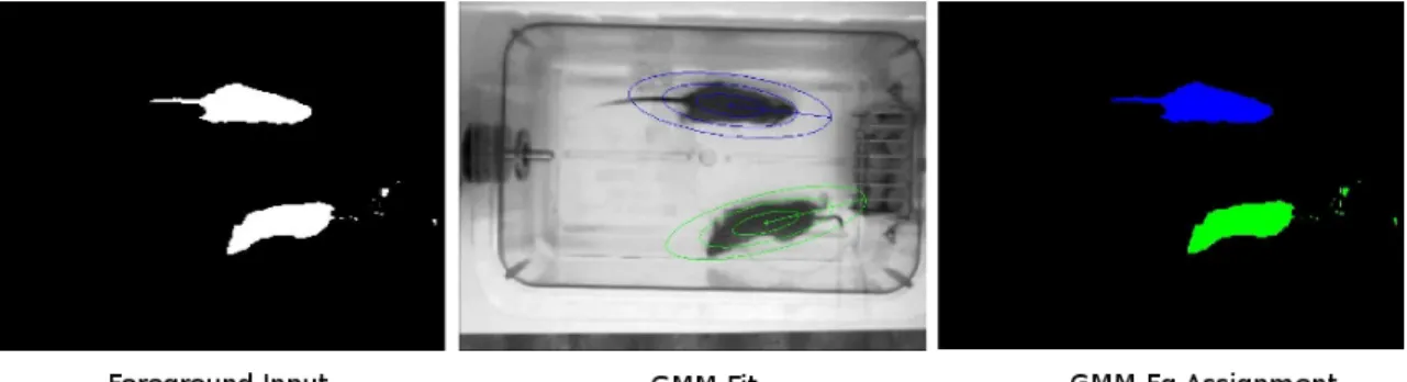
shows a sample foreground input. From this input, the EM GMM algorithm clusters the foreground. The center image shows the first three standard deviations of each cluster. Then in the right image, the foreground pixels are assigned to the highest probability cluster. . . . 34
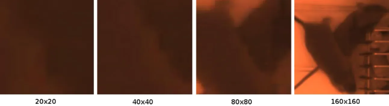
4-5 Each image from left to right doubles the patch size over the same mouse-to-mouse boundary, illustrating the challenge of detecting this boundary. In this image, the mice are approximately 220 pixels long 70 pixels wide. In the first 20 x 20 pixel crop, the mouse-to-mouse bound-ary is not visible. The mouse-to-mouse boundbound-ary becomes visually apparent only after the patch size reaches 80 x 80 pixels. . . 38 4-6 Occlusion Tracker - The figure illustrates the operation of the
occlu-sion tracker. (a) shows the current frame. (b) overlays the current foreground and the previous frame’s ellipses. In (c), the upper-right mouse’s new foreground is computed using the ellipse overlap condition from equation 4.13 coupled with a largest connected component algo-rithm. Then an ellipse is fit to the boundary of this mouse’s computed foreground. The computed foreground and ellipse fit for the lower-left mouse are not shown. . . 39 4-7 The figure illustrates an error with the occlusion tracker. (a) shows
the current frame. (b) shows the ellipse track of mouse 1 spanning two mice. (c) shows mouse 2 with an oversized foreground and an ellipse track clearly spanning two mice. . . 40 4-8 Examples illustrating the complete tracking system. The top frame
shows the original frame and the below frame shows the results of complete tracking system. . . 42 4-9 Examples illustrating the three tracking scores. The top frame shows
the original image, and the bottom frame shows the tracks. For the tracks scored 1, both ellipse tracks follow the mouse boundaries; for the tracks scored 2, both tracks are centered over each mouse, but the left mouse’s track incorrectly includes the head of the other mouse; and for the tracks scored 3, both tracks clearly span multiple mice. . 43
4-10 Examples illustrating the three orientation scores. The top frame shows the original image, and the bottom frame shows the tracked orientations. For the left frame with an orientation score of 0, both el-lipse orientations are correct; for the middle frame with an orientation score of 1, one of the orientations is incorrect; and for the right frame with an orientation score of 2, both orientations are incorrect. . . 44 5-1 The number of frames for each of the four social behaviors in the test
set. The mapping from numbers to behavior labels is as follows: 2 = NN, 3 = NH, 4 = NA, 5 = U. . . 52 5-2 The number of frames for each of the four social behavior in the training
set. The mapping from numbers to behavior labels is as follows: 2 = NN, 3 = NH, 4 = NA, 5 = U. . . 53 5-3 Each linear kernel classifier is tested on its left-out training data, and
the resulting confusion matrix is calculated by averaging all 10 tests on the left-out training data. . . 56 5-4 Each gaussian kernel classifier is tested on its left-out training data,
and the resulting confusion matrix is calculated by averaging all 10 tests on the left-out training data. . . 57 5-5 Confusion matrix for the linear kernel averaged across all 10 test videos. 57 5-6 Confusion matrix for the gaussian kernel averaged across all 10 test
videos. . . 58 5-7 Confusion matrix containing the social behaviors lumped into one class
and the background class for the linear kernel averaged across all 10 test videos. . . 59 5-8 Confusion matrix containing the social behaviors lumped into one class
and the background class for the gaussian kernel averaged across all 10 test videos. . . 59
List of Tables
3.1 The mouse social behaviors annotated in the dataset. Relevant defini-tions from Defensor et al. [9] are repeated for completeness. . . 25 4.1 The average tracking scores for the EM GMM tracker and the occlusion
tracker. . . 45 4.2 The average number of incorrect orientations for the EM GMM tracker
and the occlusion tracker . . . 45 5.1 The feature representation for the behaviors. Mouse i refers to the
mouse represented by this feature vector, and mouse j refers to the other mouse. . . 51 5.2 Total performance, number of frames classified correctly / number
frames, averaged for all 10 test videos. . . 58 5.3 The predicted and labeled average number of sequences for each
behav-ior averaged across all 10 test videos. The prediction uses the results from the linear kernel. The results from the gaussian kernel are similar, but include fewer predicted sequences instances. . . 60
List of Algorithms
Chapter 1
Introduction
When studying human disorders including Parkinson’s, Epilepsy, depression, and autism, biologists develop mouse models of these human disorders in order to inves-tigate potential causes and cures [22, 9, 20, 18, 17]. For instance, biologists may hypothesize a specific gene leads to autistic-like symptoms, and by suppressing the activity of that gene, the autistic symptoms can be mitigated. To test this hypothesis, biologists may create a mouse line with this gene mutation. Evaluating the efficacy of this mouse line as a model for autism requires a quantitative assessment of mouse behavior.
Human behavioral assessment, the primary means for assessing behavior in mouse models, cannot keep up with the growth in the field. New mouse lines and experiments are created faster than the capacity of human behavioral analysis [33]. The time scales of manual behavior assessment are expressed in minutes instead of days, and thus lack the statistical power of long-term study. The short time scales stem from the painstaking manual video analysis needed to reliably assess mouse behavior.
Automated behavioral analysis addresses the problems of time, cost, and repro-ducibility inherent to human behavioral analysis. Due to these problems and due to the relatively controlled laboratory environment inhabited by mice, much research has gone into establishing automated systems to phenotype mouse behavior. Early techniques employed sensors capable of assessing position, coarse movements, and instances of specific actions including eating and drinking [11, 32]. More recently,
computer vision systems have been developed to support more flexible and complex behavior analysis. One of the most advanced systems developed by Jhuang et al. [14] for singly housed mice detects fine-grained behaviors such as grooming and can be trained to recognize new behaviors from annotated videos.
For human diseases with a social component such as depression and autism, mouse models for these social disorders must include a social component as well. The com-plex interactions between mice present significant challenges for building automated systems. Mice frequently occlude one another, move erratically, and have identical appearances. Despite these challenges, automating the analysis of social behaviors empowers researchers to more quickly and effectively study human disorders that have a significant social component, and in the process, accelerate the path to cures for these social disorders in humans.
Beyond studying social disorders, a system for studying multiple mice would ben-efit long-term health monitoring. Mice naturally live in groups, so over the long-term, most mice are housed in groups to promote healthy mental conditions. Therefore, any system which monitors mice for days or even weeks needs to be capable of monitoring multiple interacting mice.
More broadly, mice provide a controlled laboratory environment to begin explor-ing the questions of how to best quantify social behavior in mice and eventually in humans. Understanding human social behavior requires comprehension of many fac-tors including facial expressions, body language, and spoken language. In contrast, mice live in controlled laboratory environments and exhibit relatively simple social behavior such as sniffing, following, and huddling. These conditions simplify many of the associated computer vision and representational challenges. Automating social behavior analysis is an important step towards developing a quantitative understand-ing of the connections between social behavior and intelligence in mice, humans, and other animals.
1.1
Contributions
In this thesis, I develop a computer vision system to automatically recognize mouse social behavior. The following describes the major contributions:
1. Mouse tracking and social interaction dataset
(a) Collected a dataset consisting of 22 ten minute recordings of two interacting mice. Two synchronized cameras film all recordings simultaneously from the top-view and side-view perspectives. The top-view is most informative for tracking and parts recognition, and the side-view is most informative for recognizing fine-grained behaviors such as grooming.
(b) Introduced a dataset containing continuous annotations of five mouse social behaviors: nose-to-nose sniffing, nose-to-head sniffing, nose-to-anogenital sniffing, crawl under / crawl over, and upright head contact. The dataset is designed to evaluate and encourage mouse social behavior research. 2. Tracker for multiple identical mice
(a) Proposed a mice detection scheme based on background subtraction and color clustering.
(b) Developed a novel top-view ellipse tracker which addresses the challeng-ing task of trackchalleng-ing multiple identical, deformable mice through complex occlusions.
(c) Developed an orientation tracker based on motion cues alone.
(d) Evaluated the ellipse and orientation trackers on data containing a wide range of mouse interactions.
3. Trainable system to automatically phenotype mouse social behaviors (a) Proposed 14 spatial features for representing mouse social behavior. (b) Developed a RLS-based [23] classification system to phenotype four mouse
(c) Evaluated the classification system over continuously annotated videos containing these social behaviors.
1.2
Outline
In Chapter 2, I provide a detailed description of related work relevant to single mouse behavior recognition and to automatic recognition of social behavior in mice, flies, and other animals. In Chapter 3, I discuss the dataset collection and annotation process for the new mouse social behavior dataset. In Chapter 4, I describe the system developed to detect and track multiple identical mice. Once the mice are tracked, the tracks are transformed into a representation suitable for classification. In Chapter 5, I detail the feature representation and the classification techniques applied to recognize social behavior. In Chapter 6, I conclude with a discussion of future work and a summary of the thesis’s contributions.
Chapter 2
Background and Related Work
2.1
Automated Mouse Behavioral Phenotyping
The controlled laboratory environment and the prominent role of mice in biological research has stimulated significant interest in automating mouse behavioral pheno-typing. Approaches range from primitive sensors to detect eating and drinking to more sophisticated computer vision systems capable of detecting behaviors such as grooming and sniffing. This section reviews the various approaches to phenotyping mouse behavior.
2.1.1
Single Mouse Systems
Most early approaches to automating mice behavioral analysis relied on sensors. Sen-sors systems include cages outfitted with photobeams and capacitance senSen-sors to detect eating and drinking [11], and infrared sensors to detect active versus inac-tive periods [32]. The sensor-based approaches are limited in the complexity of the behaviors they can represent. Sensor-based approaches are well suited for assessing position in the cage and for addressing coarse movements, but they are not suited for measuring more fine-grained behavior such as grooming and sniffing.
Advances in visual tracking techniques have led researchers to design a variety of based systems for automating mouse behavioral phenotyping. Most
vision-based approaches rely on visual tracking features [28]. Visual tracking features enable these systems to track the position of the mouse over time; however, these systems lack the ability to analyze fine-grained behaviors such as grooming and sniffing. As part of the Smart Vivarium project [2], Doll´ar et al. [10] developed the first sys-tem capable of analyzing fine-grained behaviors in the home-cage environment. The system computed spatio-temporal interest point descriptors to represent five basic behaviors: eating, drinking, grooming, exploring, and resting. Using a computa-tional model of motion processing in the primate visual cortex, Jhuang et al. [14] achieved state of the art performance on Doll´ar et al.’s five behaviors and applied this model to achieve human level performance for eight mice behaviors: drinking, eating, grooming, hanging, micromovement, resting, rearing, and walking. HomeCageScan, a commercial system developed by Cleversys Inc., recognizes a wide range of mouse behaviors and has been used in a variety of behavioral studies [25, 30]. In the evalu-ation of Jhuang et al. [14], the authors’ system outperformed HomeCageScan across these eight stereotypical behaviors.
2.1.2
Mouse Social Behavior Systems
Recent interest in long-term mice health monitoring and in social disorders such as autism has created a need to automate the analysis of mouse social behavior. In contrast to the rapid innovation seen in visual tracking for singly housed mice, there has been relatively little work automating the analysis of mice social behavior. As part of the Smart Vivarium project, the researchers developed trackers for multiple mice [4, 5], but did not apply these trackers to social behavior analysis. For measuring social approach, Pratte and Jamon [22] tagged three mice with fluorescent paper and tracked the distances between the papers with Noldus Ethovision [28]. Nadler et al. utilized photocell break-beam sensors to measure the time mice spent together in each chamber. In other recent studies, researchers computed visual statistics ranging from the distance between center of mass points [12] to number of connected components [17]. These coarse visual features indicated how often two mice interacted. Two commercial systems, SocialScan [13], a commercial system developed by Cleversys
Inc., and Ethovision XT, a commercial system developed by Noldus Inc., perform social behavior tracking from a top-view configuration. Both systems claim to be able to assess social behaviors including nose-to-nose and nose-to-tail interactions.
2.2
Automated Social Behavior Phenotyping in Other
Animals
Automated social behavior analysis of animals other the mice has also generated sig-nificant research interest. Research in this field is very diverse, ranging from vision-based social behavioral analysis of zebrafish [21] to a stereo vision system for recon-structing the motion from honey bee clusters [16]. The section describes recent ant and Drosophila (fly) social behavior literature most relevant to this thesis.
In a study of ant social behavior [1], researchers developed a system to track a large group of interacting ants using an MCMC-based particle filter [35]. The system identified three ant social behaviors: head-to-head, head-to-body, and body-to-body encounters. From the data, the researchers concluded that ants deliberately avoided encounters with other ants and performed head-to-head encounters at a statistically higher rate than other encounter types. Although the system performed quite well, the MCMC-based particle filter relies on a rigid target assumption which is not applicable to highly deformable mice.
Recent successes in automating Drosophila social behavior offers inspiration for fu-ture social behavior research. In [8], the authors developed a computer vision system to quantify Drosophila actions associated with courtship, aggression, and locomo-tion. Sample behaviors include aggressive tussling, courtship, lunging, circling, and copulation. The behaviors were represented in terms of Drosophila spatial features such as velocity, acceleration, relative head-to-head orientation, and change in orien-tation. For most behaviors, an expert manually selected the appropriate parameters ranges to classify each behavior, resulting in 90 − 100% detection rates. For certain complex behaviors such as lunging, a combination of expert selection and a k
-nearest-neighbor classifier proved to be sufficient. In subsequent work by Branson et al. [6], the authors developed an automated computer vision system to track and identify fly behavior. The behavior set included walking, backing up, touching, jumping, and other relatively simple behaviors. As in [8], the behaviors were represented in terms of spatial features such as velocity, relative angles, and relative distances. Instead of having trained experts specify parameter ranges, the system learned parameter ranges from representative videos of each behavior. The parameter range selection applied a genetic algorithm to minimize a cost function involving missed detections, spurious detections (false positives), and mislabeled frames.
Drosophila behavior definitions based on parameter ranges have the advantage of interpretability over traditional machine learning systems. When a behavior is clas-sified in terms of parameter ranges, a researcher can grasp why the system clasclas-sified a frame, and correct or refine the parameter ranges to suit a particular experiment. Although interpretable, parameter ranges fail to capture more complex behavior like fly lunging. Furthermore, the rigid fly shape lends itself to parameter intervals, which may not be appropriate for a deformable mouse.
Chapter 3
Mouse Social Behavior Dataset
Most existing mouse behavior datasets record singly housed mice in the home-cage environment [14]. In order to phenotype mouse social behavior, I needed to collect a new mouse social behavior dataset to train and evaluate the system. Any dataset has two competing goals. On one hand, the dataset should be representative of the desired test conditions. In this case, the test conditions constitute real cages where mice are interacting. On the other hand, too much environmental variability runs the risk of making a system overly complex and infeasible to design without significant technical advances. In this chapter, I describe the process of collecting and annotating a mouse social behavior dataset and discuss how the challenges of mice tracking factored into the dataset collection process.
3.1
Previous Mouse Datasets
The UCSD Smart Vivarium project [2] sought to develop the computational tools for recognizing mouse behavior. Through this project, the first mouse datasets became available. Branson et al. collected video clips to develop a tracker for multiple mice [5, 4]. Doll´ar et al. created a dataset consisting of 406 one to ten second clips containing five mouse behaviors: drinking, eating, exploring, grooming, and sleeping [10]. More recently, Jhuang et al. collected and annotated 4200 short clips (approximately 2.5 hour of videos), and over 10 hours of continuously annotated videos of eight mouse
behaviors [14]. None of these available datasets include annotations for mouse social behavior.
3.2
Affect of Mice Tracking Challenges on Data
Collection
In a common behavioral experiment, experimenters assess the difference between a wild-type and mutant strain. Typically, the mutant strain varies from the wild-type strain by a single gene mutation or alteration. As a result, the strains have nearly identical appearances. The identical appearances complicate tracking and detection. During close interactions and occlusions, mice identities are hard to distinguish. While mice do frequently occlude from the side-view perspective, mice occlude far less often from the top-view perspective. When the mice are occluding in the top-view per-spective, there is often a side-view perspective in which the mice are not occluding and vice versa. As a result, the dataset uses two frame-synchronized cameras record-ing simultaneously from the top-view and side-view of the cage. Although due to time and complexity constraints the system only incorporates the top-view perspec-tive, I expect that fusing information from both perspectives will improve tracking performance.
Since the mice look nearly identical, markers are needed to distinguish mouse identities at the end of each experiment. Previous experiments have used mouse markers to distinguish mice with similar sizes and fur color. For 1−2 day experiments, livestock markers can be used to paint blobs; for short-term experiments, permanent markers, highlight markers, or colored flourescent tags illuminated with UV light are sufficient; and for longer-term experiments, mice can be dyed with brightly colored human hair dye [28]. Certain markers, such as permanent marker pens or paint blobs, have smells or colors which could impact behavior. To reduce the chance of markers impacting behavior, one mouse’s tail in each experiment is marked with a simple water-based black marker. This enabled the experimenter to identify the mouse
identities at the end of each experiment. Even if the automated detection system could identify a mouse’s tail pixels, the black marker’s color was not sufficiently distinctive from the other dark brown mouse colors to reliably identify the black marker with the automated system. As a result, the automated system does not use the black marker to resolve identities.
3.3
Data Collection
The MIT Committee of Animal Protocol (CAC) approved all experiments involv-ing mice1. All experiments recorded the first 10 minutes of interaction for pairs of
C57BL/10J background mice. To capture peak activity, all recordings occurred dur-ing the night cycle. At a distance of a few feet from the cage, 250W Damar Red bulbs brightly illuminated the cage. Red illumination was selected because the mouse visual system cannot perceive red.
All recordings used two Point Grey Research Firefly MV color cameras connected to a PC workstation (Dell) by means of Firewire 1394b 15ft cables. One camera was mounted on a tripod facing the side of the cage, and the second camera was mounted from a custom structure facing down to the top of the cage. Both cameras wrote compressed 640x480 video at 30 fps and operated on the same Firewire bus. Using the Point Grey Research software API, I wrote custom software to frame-synchronize the two cameras streams.
n = 22 recordings of pairs of C57BL/10J background mice with nearly identical brown coats were recorded. To maintain mouse identities, one mouse’s tail in each video was marked with a water-based black marker. Each recording included two simultaneous, frame-sychronized recordings from the top-view and side-view of the cage (2 videos per recording x 22 recordings = 44 videos). Each video recording lasted for at least 10 minutes. For each recording, two mice were transferred simultaneously from a singly housed cage to the recording cage. A mouse was never used in more than two recordings.
3.4
Dataset Annotations
The 10 minute videos were annotated with two types of annotations: social behaviors and mouse part labels.
3.4.1
Social Behavior Annotation
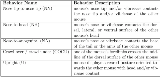
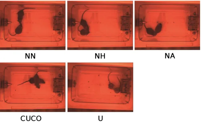
A mouse behavior expert annotated 12 of the 22 videos with social behaviors. The annotated behaviors followed the study of Defensor et al., in which the authors studied social avoidance and gaze aversion-like behavior in BTBR T+ tf/J mice [9]. The mouse behavior expert annotated the five social behaviors defined by Defensor et al.: nose tip-to-nose tip (NN), nose-to-head (NH), nose-to-anogenital (NA), crawl under / crawl over (CUCO), and upright (U). The relevant behavior definitions are repeated in Table 3.1, and Figure 3-2 shows sample images of each behavior.
When studying these behaviors, the behavior researchers compare mouse strains to draw broader conclusions about mouse behavioral patterns. For instance, in the Defensor et al. study, BTBR, a mouse studied as a model for autism, exhibited an avoidance of frontal reciprocal orientations, which the authors claim is a mouse analogue to human gaze avoidance [9]. In terms of the defined behaviors, BTBR exhibited decreased frontal behaviors (NN,NH,U) and increased avoidance of frontal behaviors (NA, CUCO). Automatic, quantitative assessment of these behaviors would allow researchers to perform this study faster and more reliably across many more mouse strains.
3.4.2
Parts Annotation
Accurate identification of mouse parts, such as the head, body, and tail, is important for classifying social behavior. Mistaking the head for the tail could cause nose-to-nose sniffing to be classified as nose-to-anogenital sniffing. To support the development of accurate mouse parts classification algorithms, I annotated 118 frames sampled randomly from the mouse recordings and sampled equally from the top-view and the side-view perspectives. In each sampled frame, I separately annotated the head,
Behavior Name Behavior Description
Nose tip-to-nose tip (NN) mouse’s nose tip and/or vibrissae contacts the nose tip and/or vibrissae of the other mouse
Nose-to-head (NH) mouse’s nose or vibrissae contacts the dor-sal, lateral, or ventral surface of the other mouse’s head
Nose-to-anogenital (NA) mouse’s nose or vibrissae contacts the base of the tail or the anus of the other mouse Crawl over / crawl under (COCU) one of the mouse’s forelimbs crosses the
mid-line of the dorsal surface of the other mouse Upright (U) mouse displays a reared posture oriented to-wards the other mouse with head and/or vib-rissae contact
Table 3.1: The mouse social behaviors annotated in the dataset. Relevant definitions from Defensor et al. [9] are repeated for completeness.
body, and tail of each of the two mice using the LabelMe annotation software [26]. For each mouse part, I annotated the polygon enclosing each part. Figure 3-1 shows a sample parts annotation. The images included a range of occlusions, so in some images, occlusions prevented all parts of both mice from being labeled.
Figure 3-1: The left image shows the original image, and the right image illustrates the corresponding head, body, and tail parts annotation.
3.5
Conclusions
In this chapter, I presented a method for simultaneously recording mice from multiple perspectives. Using this method, I recorded n = 22 mice pairs for 10 minutes
simulta-Figure 3-2: Sample images of all five annotated behaviors as described in Table 3.1. neously from both a top-view and a side-view perspective. These videos were used to create a mouse parts dataset supporting the development of mouse parts detectors, and a mouse social behavior dataset for training and evaluating machine learning algorithms to recognize mouse social behavior. While this dataset collection and an-notation was essential to developing this system, the hope is that publicly releasing the dataset encourages other researchers to improve the algorithms and methods pre-sented in this thesis. In future work, the top-view and side-view perspectives will be combined to improve performance. The top-view is most informative for tracking and parts identification, and the side-view is most informative for recognizing fine-grained behaviors such as grooming.
Chapter 4
Mice Tracking
Classifying mice social behavior requires a computer vision system capable of detect-ing and trackdetect-ing the mice in each frame. Solvdetect-ing the mice trackdetect-ing problem reduces to the very challenging problem of tracking multiple, textureless, near-identical de-formable objects. Unlike traditional single target phenotyping, social behavior phe-notyping is most interested in the interactions between targets, but at the same time, these close interactions are the most difficult tracking problems. In this chapter, I describe the challenges of tracking multiple mice and propose a tracking system to address these challenges.
4.1
Challenges of Tracking Mice
Many computer vision techniques for detection and tracking do not translate to the mice tracking problem. Figure 4-1 illustrates a set of representative frames demon-strating the mouse tracking challenge. The following details the primary mice tracking challenges:
• Complex Occlusions - mice walk over one another, roll around each other and interact in many complex ways. These occlusions reduce the signal available to the tracker.
points (e.g. SIFT [15]) are not reliable over many frames due to self-occlusion and occlusions between mice.
• Highly Deformable - mice deform into many shapes, sizes, and orientations. Consequently, sliding window object detection systems are not effective for de-tecting and tracking mice.
• Long-Term Tracking - the system must track over long-term experiments with minimal human intervention; otherwise, the system is unlikely to be adopted by the research community.
• Identical Appearances - people typically wear different clothing or exhibit other dissimilarities which can be distinguished using simple appearance models such as a color histogram. In contrast, mice have identical appearances, which makes appearance a weak cue for resolving pixel identities during mice interactions. • Unpredictable Motion - mice move erratically and change directions abruptly.
This complicates the use of motion models to predict future mouse locations.
4.2
Tracking System
The tracker design accounts for two primary constraints: fully automated operation and a requirement that there are always k tracks, where k is the number of mice. The fully automated operation constraint ensures that the tracks are acquired fully automatically and recover from any errors without human intervention. The k tracks constraint ensures the system generates track hypotheses for all mice even during the most complex interactions. Notice the constraints do not include real-time operation and strict identity maintenance. Removing the real-time constraint allows the tracker to leverage past and future information and to employ algorithms which would not be computationally feasible in a real-time setting. Not requiring strict identity main-tenance addresses the reality of mouse tracking: certain interactions (e.g. fighting) are so complex that identity tracking cannot be assured.
Figure 4-1: Representative frames illustrating challenging tracking sequences. Refer to Algorithm 1 for a concise overview of the entire mice tracker operation. Section 4.2.1 provides an overview of the tracker. In the subsequent sections, I de-tail the implementation of each subcomponent. Section 4.2.2 describes the mouse detection system based on background modeling techniques. Then in Section 4.2.3, I describe the tracker designed for physically separated mice. Section 4.2.4 discusses the process for detecting occlusions, and once an occlusion is detected, Section 4.2.5 de-scribes the tracker designed to operate during mouse occlusions. Section 4.4 presents detailed performance metrics for the entire tracking system.
4.2.1
Tracking System Overview
The mice tracking system consists of three major components: a mouse detection sys-tem, a tracker outside of occlusions, and a tracker during occlusions. A non-adaptive background model is a simple yet effective technique for detecting candidate mouse
lo-bg ← generateBg(videoFn); 1 isOcclusion ← false; 2 ellipses ← empty; 3
while ( frame = getNextFrame( videoFn)) do
4
% Section 4.2.2 ;
5
fg ← computeFg(frame,bg) ;
6
if not isOcclusion then
7 % Section 4.2.3 ; 8 clusterLabels ← gmmCluster(fg,ellipses) ; 9 [fg connectLabels] ← connectedComponents(fg,clusterLabels) ; 10 else 11 % Section 4.2.5 ; 12 [fg connectLabels] ← occlusionConnectedComponents(fg,prevEllipses); 13 end 14
ellipses ← fitEllipsesToConnectedComponents(fg, connectLabels);
15
% Section 4.2.4 ;
16
fisherCriteria ← computeFisherCriteria(ellipses);
17
isOcclusion ← not ellipsesIdentical(ellipses) and fisherCriteria < αocc; 18
end
19
Algorithm 1: The operation of the mice tracker.
cations. Since lighting conditions are known and constant, the background is approx-imately constant throughout an entire video. A static background is thus sufficient for detecting the hypothesized foreground locations. Once the hypothesized fore-ground locations are identified, a Gaussian Mixture Model (GMM) [3, 29] forefore-ground clustering algorithm effectively tracks the mice outside occlusions. Once clustered, a largest connected component algorithm combined with the morphological open oper-ation selects the mouse pixels in each cluster. When the mice are closely interacting or occluding, GMM clustering does not result in good mouse segmentations. Unable to develop an algorithm to reliably detect the contour between interacting mice, I instead developed an occlusion tracker which leveraged each mouse’s previous loca-tion and a known mouse size. Although this technique did not accurately maintain identities through all interactions, the technique handled many complex interactions and occlusions.
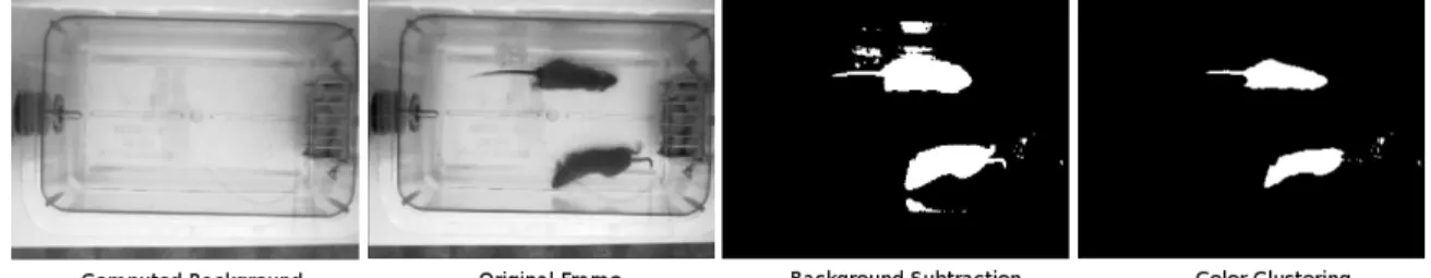
Figure 4-2: Identifying mouse foreground pixels - The current frame is subtracted from the background model and pixels above a threshold τ are classified as foreground. Color clustering cleans the foreground further by removing lighter colored pixels.
4.2.2
Background Modeling
Background subtraction generates a model of the cage background ybg, which removes
instances of moving objects (leftmost image in Figure 4-2). In the mouse dataset, the dark brown mice are darker than the rest of the background. Under this assumption, the background model is generated using the following algorithm:
1. Sample 100 frames distributed throughout the video.
2. Represent each pixel by a 100-dimensional vector consisting of one intensity value from each of the 100 sampled frames.
3. Use k-means with 2 clusters independently for each pixel’s feature vector. Select the brighter cluster center as the background cluster.
To generate the hypothesized foreground pixels for each frame observation yt,
subtract the current frame observation yt from the background model ybg. Values
higher than a certain threshold are labeled as foreground (second from right in Figure 4-2). Formally, let τ be the foreground threshold and let yf g be the resulting binary
foreground image defined by the following equation:
yf g = ybg− yt< τ (4.1)
Since the mice are filmed from a static camera in a controlled indoor environment, the assumptions of a static background and fixed camera generally hold. As a result,
this algorithm generates a robust background. The second image from the right in Figure 4-2 illustrates a sample result of this method.
Problems with Background Subtraction Background modeling has a few defi-ciencies:
• Mouse colored background pixels - when nearly all the frame samples contain a mouse at a given pixel location, the background value at this pixel locations will be mouse colored.
• Sensitivity to free threshold parameter τ - if τ is set too high, not enough of the mouse is classified as foreground, and in contrast, if τ is set too low, too many background pixels are classified as foreground.
• No identity information - the resulting foreground only produces candidate mouse pixels and does not provide mouse identity labels for those foreground pixels.
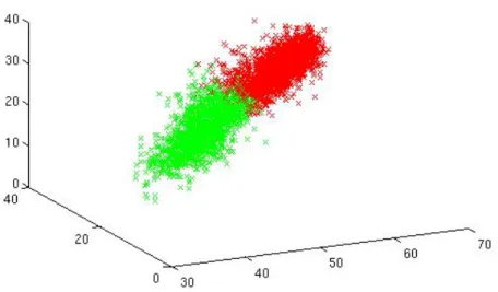
The first deficiency, mouse colored background pixels, can typically be solved by either sampling over more frames, or by sampling over a frame range when the mice are very active. The third deficiency, no identity information, is not handled as part of the foreground computation layer; rather, the identity information is inferred by the clustering algorithm described in Section 4.2.3. The second deficiency, sensitivity to the free threshold parameter τ , is mitigated by color clustering. The following details the procedure to improve background subtraction with color clustering: Color Clustering to Improve Background Subtraction Color clustering re-duces background subtraction’s sensitivity to the free parameter τ . When performing color clustering, τ is set to a low value in order to generate an excess number of hy-pothesized foreground pixels. Color clustering then selects the foreground pixels more likely to be mouse colored. Figure 4-3 shows the result of color clustering. The darker pixels are more likely to belong to a mouse, so the color clustering selects the darker cluster, the cluster closest to (0, 0, 0), as the mouse cluster. In many instances such
as in Figure 4-2, the color clustering removes many reflections, because the reflections are lighter colored than the mouse. The following describes the procedure for color clustering:
1. Convert the color frame to CIELAB. The CIELAB color space is designed to approximate the color perception of human vision [31].
2. Apply background subtraction to generate a set of hypothesized foreground locations, yf g.
3. Represent each foreground pixel with its three-dimension color vector.
4. Cluster all the foreground pixels’ color vectors into two color clusters using k-means.
5. Since the mice are dark colored, all the foreground pixels assigned to the darker cluster (closer to (0, 0, 0)) are assigned as mouse foreground, ymouse, and the
rest are assigned as background.
Figure 4-3: Sample result of color clustering on the foreground pixels. The mouse cluster is shown in green and the background cluster is shown in red. The plot illustrates that color clustering selected the dark pixels, the pixels cluster closest to (0, 0, 0) in the CIELAB color space.
4.2.3
Tracking Outside of Occlusions
Given the hypothesized foreground locations from the background modeling phase, these foreground locations must be assigned to the k mouse identities. Foreground pixels are assigned to mouse identities using two simple operations. First the fore-ground pixel locations are clustered using the Expectation Maximization (EM) algo-rithm applied to a k-cluster Gaussian Mixture Model (GMM) [3]. Figure 4-4 shows an example of this clustering. Once clustered, a morphological open operation removes some isolated foreground pixels. Then a connected component algorithm processes each cluster, and the largest connected component in the cluster is labeled as the mouse.
Figure 4-4: EM GMM foreground clustering outside of occlusions. The left image shows a sample foreground input. From this input, the EM GMM algorithm clusters the foreground. The center image shows the first three standard deviations of each cluster. Then in the right image, the foreground pixels are assigned to the highest probability cluster.
EM GMM foreground clustering This section describes the algorithmic details of the EM GMM foreground clustering. The algorithm closely follows the formulation in [3]. Let X be an n x 2 feature matrix containing the n foreground pixels, and let k be the number of mice to track. Each foreground pixel, xi, is represented by its
(x, y) image location. The EM algorithm alternates until convergence between an expectation step (E step) and a maximization step (M step).
In the E step, the means, µj’s, and covariances, Σj’s, for each cluster j are given
in each cluster. The weight, wij, of point xiin cluster j is computed from the cluster’s Gaussian pdf: wij = 1 2π|Σj| 1 2 exp(−1 2(xi− µj) TΣ−1 j (xi− µj)) (4.2)
Each point’s weights are then normalized to sum to one. In this way, each point’s cluster membership is a valid pdf. Formally, the new normalized weight, ˜wij, of point
i in cluster j is computed as:
˜ wij = wij Pn j=1wij (4.3)
In the M step, the means (µj’s) and covariances (Σj’s) are updated using the new
normalized weights: µj = Pn i=1w˜ijxi Pn i=1w˜ij (4.4) Σj = Pn i=1w˜ij(xi− µj)(xi− µj)T Pn i=1w˜ij (4.5)
This process alternates between the E-step and the M-step until the log-likelihood, L, converges below a given threshold. The log-likelihood L is averaged across all k mouse clusters: L = k X j=1 1 klog( n Y i=1 ˜ wij) (4.6) = 1 k k X j=1 n X i=1 log( ˜wij) (4.7)
One weakness of EM algorithm is the algorithm’s susceptibility to local minima. Two steps are in place to avoid local minima. On the first iteration, the cluster means and covariances are initialized using k-means. On subsequent iterations, the previous frame’s means (µj’s) and covariances (Σj’s) initialize the EM search in the current
frame. Seeding the means and covariances with these values generally results in good cluster fits.
4.2.4
Detecting Occlusion Events
Detecting occlusion events requires finding a good measure for distance between the mouse pixel distributions. One simple solution for detecting occlusion events is to compute the distance between mouse cluster centers and then to set an empirical dis-tance threshold for detecting occlusions. If mice were spherical, this solution would perform well. However, as evident from the center image in Figure 4-4, mice pixels distributions are typically elliptical. Fisher’s linear discriminant helps address the problem of computing the distances between distributions with non-spherical covari-ances. Fisher’s linear discriminant selects a projection w from the D-dimensional data space onto single dimensional space that maximizes the distance between the two classes while minimizing the covariance within each class. It does this by max-imizing Fisher’s criterion, J (w), the ratio of the between-class variance, SB, to the
within-class variance, SW [3]: J (w) = w TS Bw wTS Ww (4.8) The maximal value of J (w) can be used as distance metric between non-spherical distributions. In terms of two class means, µ1 and µ2, and two class covariances, Σ1
and Σ2, the Fisher criterion can be maximized to produce Fisher’s linear discriminant
as follows [3]: SB = (µ2− µ1)(µ2− µ1)T (4.9) SW = Σ1 n1 +Σ2 n2 (4.10) w ∝ Sw−1(µ2− µ1) (4.11)
Defining the maximal value of J (w) to be the distance between the classes, I define J (w) < αocc as the criterion for mice entering an occlusion state. In order to
calculate the maximal J (w), I must express the connected component of each mouse in terms of a mean, µ, and a covariance, Σ. To achieve this, an ellipse is fit to the boundary pixels of each connected component. The center of the ellipse defines the µ. Σ is computed from the ellipse parameters θ, the rotation from the x-axis; a, half the
ellipse x-axis length after rotation; and b, half the ellipse y-axis length after rotation. Let R be the rotation matrix in terms of θ. Then a basic relation exists to convert ellipse parameters to a covariance Σ:
Σ = R a2 0 0 b2 RT (4.12)
Once Σ and µ are found for each cluster, the maximal J (w) < αocc can be
calcu-lated pairwise for all clusters to determine when two mice enter an occlusion state.
4.2.5
Tracking During Occlusions
During occlusions and close interactions, standard segmentation and contour detec-tion algorithms cannot reliably detect the boundaries between the mice. Figure 4-5 illustrates the challenge of identifying this boundary. Human observer can only iden-tify the mouse boundary locations after the patch size grows very large. At least qualitatively, the large amount of context required to discern the boundary suggests that the human visual system relies on high-level contour or model information to detect the boundary between mice. This observation may explain why boundary de-tection techniques could not detect this boundary. Boundary dede-tection techniques typically represent the boundaries in terms of local luminance, chrominance, and tex-ture differences, but for the boundary between mice, these local differences are weak or nonexistent.
Since I could not reliably detect the boundaries between mice, the occlusion tracker leverages a set of simple heuristics that generally perform well without any input about the mouse-to-mouse boundaries. The occlusion tracker makes two major as-sumptions: both mice can be modeled by a fixed sized ellipse, and a mouse’s previous ellipse location is a good cue for the mouse’s current location. Once an occlusion event is detected by the criterion described in Section 4.2.4, the occlusion tracker begins to track the mice.
Figure 4-5: Each image from left to right doubles the patch size over the same mouse-to-mouse boundary, illustrating the challenge of detecting this boundary. In this image, the mice are approximately 220 pixels long 70 pixels wide. In the first 20 x 20 pixel crop, the mouse-to-mouse boundary is not visible. The mouse-to-mouse boundary becomes visually apparent only after the patch size reaches 80 x 80 pixels.
ellipse models from the previous frame to assign foreground pixels to each mouse in the current frame. For each mouse i, the occlusion tracker calculates Mi,t, the set of
hypothesized foreground pixels for mouse i at time t. Mi,t is initialized to F Gt, the set
of all foreground pixels at time t. The occlusion tracker discards all foreground pixels from Mi,t which overlap with another mouse’s, i 6= j, previous ellipse, and do not
overlap with the current mouse’s previous ellipse. Foreground pixels are permitted to be assigned to multiple mice. Formally, let Ei,t−1 be the set of pixels covered by
the previous ellipse of the ith mouse, k be the number of mice, and D
i be the set of
integers from 1 to k excluding i. Mi,t is then defined by the following equation:
Mi,t = F Gt− ((
[
j∈Di
Ej,t−1) − Ei,t−1) (4.13)
For each set of hypothesized mouse foreground pixels Mi,t, a largest connected
component algorithm further curates the pixels in each Mi,t. Figure 4-6 illustrates
an example of the occlusion tracker applied to two closely interacting mice. The algorithm is designed so that each mouse acquires foreground pixels along its motion direction and loses foreground pixels from the places it left in the previous frame. However, sometimes the mice move in a way that causes the occlusion tracker to add pixels from the other mouse’s new locations. Figure 4-7 highlights an example in
which the occlusion tracker does not add the correct pixels.
To prevent a mouse’s ellipse track from growing too large (or too small), the occlusion tracker enforces an empirical ellipse size. First, an ellipse is fit to the boundary of mouse’s new connected component. Then assuming an accurate center for the ellipse fit, the ellipse major and minor axes are resized to the size of a standard occlusion ellipse. The standard occlusion ellipse’s major and minor axis sizes are determined by sampling many frames in which the mice are not in an occlusion state and then computing an empirical average of the major and minor axis parameters. Although this size will not be accurate in many cases such as when the mouse is reared or elongated, the size constraints enforce a primitive mouse model. The model prevents a mouse track from growing (or shrinking) to unrealistic mouse dimensions. For quantitative benchmarks of this occlusion tracker, refer to Section 4.4.
Figure 4-6: Occlusion Tracker - The figure illustrates the operation of the occlusion tracker. (a) shows the current frame. (b) overlays the current foreground and the previous frame’s ellipses. In (c), the upper-right mouse’s new foreground is computed using the ellipse overlap condition from equation 4.13 coupled with a largest connected component algorithm. Then an ellipse is fit to the boundary of this mouse’s computed foreground. The computed foreground and ellipse fit for the lower-left mouse are not shown.
4.3
Parts Tracking
The mouse tracking system produces ellipses tracks for each mouse. Although it is generally safe to assume the nose and tail are near the endpoints of the ellipse’s major axis, the ellipse model does not differentiate between nose and tail endpoints.
Figure 4-7: The figure illustrates an error with the occlusion tracker. (a) shows the current frame. (b) shows the ellipse track of mouse 1 spanning two mice. (c) shows mouse 2 with an oversized foreground and an ellipse track clearly spanning two mice. Accurate classification of sniffing behavior requires accurate identification of the nose and tail endpoints. An inaccurate nose and tail identification could misclassify a nose-to-nose (NN) interaction as a nose-to-anogenital (NA) interaction.
4.3.1
Identifying Nose, Head, and Tail Base
The orientation tracker only uses the mouse’s motion to identify the nose and tail base. The orientation trackers assigns the nose to the endpoint on the ellipse major axis which most frequently coincided with the dominant motion direction; the tail base to the opposite major axis endpoint; and the head center to a point 15% down the major axis from the nose endpoint. The 15% value is derived from an empirical average calculated over the labeled parts training data (see Section 3.4.2). The rest of this section describes the methods underlying the orientation tracker.
The orientation tracker measures which ellipse endpoint is consistently closer to the motion direction. To compute this motion assignment, the orientation tracker maintains two queues, one for each ellipse major axis endpoint. In each frame, the algorithm calculates the velocity vt at time t between the previous ellipse center
ct−1 and the current ellipse center ct. If the velocity is above an empirical motion
threshold, a score is added to each ellipse endpoint’s queue. Using the empirical motion threshold prevents noisy small motions from cluttering the queues, such as when the mouse is resting. For each endpoint i, the score calculates the euclidean
distance between the previous frame’s ellipse endpoint, pi,t−1, and the current frame’s
ellipse center, ct, multiplied by the velocity, vt. The queue stores the following scores,
si,t, for each endpoint i:
si,t = vt||pi,t−1− ct||2 (4.14)
The score measures, on average, how close an endpoint lies to the dominant motion direction. The smaller the score, the closer the endpoint is to the dominant motion direction. When the mouse moves quickly, the proportionality to velocity penalizes endpoints that are far from the motion direction. The orientation tracker assumes that the mouse is likely moving forward when it is moving quickly. The velocity term thus gives more weight to instances where the mouse is likely moving forward.
Ellipse endpoint identities must be maintained from frame to frame, so one end-point queue only corresponds to one endend-point. Endend-point identities are maintained recursively. In the current frame, each ellipse endpoint is assigned the queue of the closest previous ellipse endpoint.
Once an endpoint queue reaches a preset size, the head direction is inferred as the orientation with the lowest mean queue value. A queue having the lowest mean is interpreted as the endpoint which most often lies in the dominant motion direction. The queue size represents a tradeoff between robust orientation estimation and ro-bustness to switched endpoint identities. If the queue is very large, short instances in which the mouse quickly moves backwards will not impact the orientation inference, but this comes at the cost of the orientation tracker taking a long time to recover in the event of the endpoint identities being switched.
Occlusions present an additional complexity to this motion tracking algorithm. Since during occlusions the ellipse motion and position are less reliable, orientation scores are not added to the queue when the mouse is in an occlusion state. However, it is still important to maintain the endpoint identities, so even during occlusions, the endpoint identities are updated to match the closest endpoint from the previous frame. The need to maintain endpoint identities during occlusion is a known source of error. The unreliability of occlusion tracks can cause the mouse endpoint identities to switch.
Since the endpoint system maintains a fixed queue, the orientation tracking does recover over time. Figure 4-8 shows examples of complete tracking system including the orientation tracker. In Section 4.4, I quantitatively evaluate the results of this mouse tracking system.
Figure 4-8: Examples illustrating the complete tracking system. The top frame shows the original frame and the below frame shows the results of complete tracking system.
4.4
Results
To evaluate the complete tracking system, three separate components need to be evaluated: the EM GMM tracker outside of occlusions, the occlusion tracker, and the orientation tracker. Evaluating frame-by-frame performance over the 10 social behavior videos would be impractical. Each video is approximately 10 minutes long, which constitutes around 180, 000 frames (10 videos x 600 seconds per video x 30 fps). I chose a sampling approach to evaluate the tracker. From each of the 10 social behavior videos, I randomly sampled 50 frames from the occlusion tracker and 50 frames from the EM GMM tracker for a total of 1000 video frames ((50 occlusion tracker frames per video + 50 EM GMM tracker frames per video) x 10 videos). For each sampled frame, I overlaid the computed tracks and annotated a tracking score and an orientation score. The tracking score measured the quality of each track in terms of three possible integers: 1 - both ellipse tracks follow the mouse boundaries; 2 - both tracks are centered over the mice but at least one track does not follow the
mouse boundary; or 3 - one or both tracks span multiple mice, or fail to track at least one mouse. Figure 4-9 provides examples to illustrate each tracking score. The orientation score measures the number of incorrect orientations: 0, 1, or 2 for the two mice case in these videos. An orientation is judged as incorrect if the wrong ellipse endpoint is assigned to the nose, or if the track was too poor for the orientation to even be meaningful. Figure 4-10 provides examples to illustrate each orientation score.
Figure 4-9: Examples illustrating the three tracking scores. The top frame shows the original image, and the bottom frame shows the tracks. For the tracks scored 1, both ellipse tracks follow the mouse boundaries; for the tracks scored 2, both tracks are centered over each mouse, but the left mouse’s track incorrectly includes the head of the other mouse; and for the tracks scored 3, both tracks clearly span multiple mice.
The tracking scores paint a picture of a tracker which performs very robustly out-side of occlusions, and tracks the mouse’s general location when the occlusion tracker is active. The tracking scores are shown in Table 4.1. For 91.6% of the EM GMM tracker samples, I assigned the EM GMM tracker a tracking score of 1, indicating that the tracker almost always accurately tracked the mouse boundaries. On the other hand, the occlusion tracker most frequently received a score of 2, indicating that it tracked the mouse locations but did not accurately fit the mouse boundary.
Figure 4-10: Examples illustrating the three orientation scores. The top frame shows the original image, and the bottom frame shows the tracked orientations. For the left frame with an orientation score of 0, both ellipse orientations are correct; for the middle frame with an orientation score of 1, one of the orientations is incorrect; and for the right frame with an orientation score of 2, both orientations are incorrect.
Although the size prior is important for ensuring the occlusion tracks do not grow too large or too small, enforcing a single ellipse size resulted in poor fits in many tracking instances. Overall, relatively few tracks received a score of 3, indicating incorrect tracks. For the EM GMM tracker, only 0.4% of the samples received a score of 3, and for the occlusion tracker, only 13.4% of the samples received a score of 3.
Although the mouse tracker generally performed well, the orientation tracker fre-quently tracked the wrong orientation. Table 4.2 paints a disappointing picture of the orientation tracker’s performance. In around 50% of the sampled frames, the orientation tracker labeled at least one of the mouse orientations incorrectly for both the EM GMM tracker and the occlusion tracker. I noticed a few key instances that caused the orientation tracker to reverse endpoint identities. When the mouse rears to a vertical position and then curls back down, or when the mouse enters into certain complex interactions, the orientation tracker would sometimes swap ellipse endpoint identities. Swapping endpoint identities causes the tail base ellipse endpoint to have
the queue of motion values previously associated to the head ellipse endpoint and vice versa. Although the queue creates orientation robustness when the endpoints are correctly tracked, it introduces a time lag into the recovery when the endpoint identities are swapped. Even though the endpoint identity switch typically occurs when the occlusion tracker is active, the queue’s time lag causes the incorrect orien-tation to persist while the EM GMM tracker is active. This explains why both ellipse trackers exhibited poor orientation performance.
Tracking Performance Tracker Score Frequency EM GMM 1 91.6% EM GMM 2 8% EM GMM 3 0.4% Occlusion 1 19% Occlusion 2 67.6% Occlusion 3 13.4%
Table 4.1: The average tracking scores for the EM GMM tracker and the occlusion tracker.
Orientation Performance
Tracker Incorrect Orientations Frequency
EM GMM 0 55.4% EM GMM 1 38.8% EM GMM 2 5.8% Occlusion 0 50% Occlusion 1 37.4% Occlusion 2 12.6%
Table 4.2: The average number of incorrect orientations for the EM GMM tracker and the occlusion tracker
4.5
Conclusions
I have presented a new system for tracking multiple identical mice through complex interactions. The tracker has been evaluated over 1000 frames randomly sampled from
the mouse social behavior dataset. The tracking system performs very well outside of close interactions and nearly always has a good ellipse around each mouse’s boundary. During interactions, the mice are generally tracked, but the ellipse track does not tightly fit the mouse boundary. In contrast to the ellipse tracker, the orientation tracker is far less robust, and in around half the sampled frames, the orientation tracker labeled at least one of the mice with the incorrect orientation. Despite these deficiencies, the tracker is immediately applicable to studies requiring only coarse position statistics, or to studies in which some inaccuracy can be tolerated, such as a system working in tandem with a human observer to identify candidate social behavior instances.
Chapter 5
Automated Phenotyping of Mouse
Social Behavior
When one mouse sniffs another mouse, humans can reliably identify and classify this behavior. It is not immediately obvious how to design an automated system to per-form the same task. The automated system must solve two related problems: feature representation and classification. Feature representation selects an appropriate set of properties to represent the behaviors. When designing a feature representation, the specific behavior set determines the appropriate feature set. For instance, suppose the behavior set includes just two behaviors: moving and not moving for a single mouse. In this case, a single feature computing the change in center of mass from frame to frame would be sufficient to characterize the difference between moving and not moving. This example demonstrates that the underlying characteristics of each behavior, and more importantly, the differential characteristics between behaviors guide the appropriate feature choices. After selecting a suitable feature representa-tion, the classification system uses this feature representation to produce a behavior label for each frame. In this chapter, I discuss the challenges of phenotyping mouse social behavior and detail the system designed to phenotype mouse social behavior.
5.1
Phenotyping Challenges
Mouse social behavior phenotyping presents three primary challenges: 1. Accurate mice tracking through occlusions and complex interactions 2. Selecting an appropriate feature representation
3. Identifying an appropriate classification framework
All three challenges are tightly coupled and significantly impact the final system performance. Inaccurate tracks have a cascade effect on the system. No matter how good the feature representation and the classification framework, the representation will not be accurate if the tracks are wrong. The features that are tracked, in turn, limit the features which can be represented. For instance, if only the mouse center of mass is tracked, the distance between the mouse noses cannot be computed from the mouse centers. Section 4.1 reviews the challenging problem of tracking multiple identical, interacting mice, and Section 4.2 describes the tracking system.
Even with accurate tracks, there are many possible feature representations and classification choices. For example, the two tracks (in this case ellipses) can be used to directly compute the feature representation, or alternatively, the tracks can in-stead be used to target the computation of other features such as edge or template based features. With an unconstrained set of feature choices, it is intractable to se-lect an optimal feature representation. The final feature set choice thus involves a combination of quantitative methods, intuition, and heuristics regarding the feature representation choice that will result in good separation between the behaviors.
In this setting, the classification framework describes two inter-related choices: the classifier and the training set. The training set must be selected very carefully. A training set which covers only an aspect of the behavioral variations may not perform well on testing data containing other behavioral variations. A further complication arises from the dependency of features on tracks. The training data should only contain valid tracks; otherwise, the classifier may learn inappropriate feature ranges that are a result of tracking errors and not representative of the behaviors.