Auto-calibrated urban building energy models as continuous planning tools for greenhouse gas emissions management

(1)

Auto-Calibrated Urban Building Energy Models

as Continuous Planning Tools for

Greenhouse Gas Emissions Management

by

Shreshth Nagpal

Bachelor of Architecture

School of Planning and Architecture, New Delhi, 2002

Master of Science in Building Design, Arizona State University, 2005

Submitted to the Department of Architecture in Partial Fulfillment of the Requirements for the Degree of

Doctor of Philosophy in Architecture: Building Technology

at the

Massachusetts Institute of Technology

June 2019

The author hereby grants to MIT permission to reproduce and to distribute publicly paper and electronic copies of this thesis document in whole or in part in any medium now known or hereafter created.

Signature of Author: ____________________________________________________________________________________________________________________ Department of Architecture May 3, 2019 Certified by: _____________________________________________________________________________________________________________________________

Christoph F. Reinhart Professor of Building Technology Thesis Supervisor Accepted by: ____________________________________________________________________________________________________________________________

Nasser Rabbat Chair, Departmental Committee on Graduate Students

(2)

(3)

Dissertation committee

Christoph F. Reinhart Professor of Building Technology Massachusetts Institute of Technology Thesis Supervisor

Caitlin T. Mueller Associate Professor of Architecture & Civil and Environmental Engineering Massachusetts Institute of Technology Thesis Reader

Leslie K. Norford Professor of Building Technology Massachusetts Institute of Technology Thesis Reader

Nico Kienzl Director, New York Atelier Ten Thesis Reader

(4)

(5)

Auto-Calibrated Urban Building Energy Models

as Continuous Planning Tools for

Greenhouse Gas Emissions Management

by

Shreshth Nagpal

Submitted to the Department of Architecture on May 3, 2019

in Partial Fulfillment of the Requirements for the Degree of Doctor of Philosophy in Architecture: Building Technology

Abstract

To reduce greenhouse gas emissions associated with their buildings’ energy use, owners frequently rely on building energy models that are calibrated to existing conditions for evaluation of potential energy efficiency retrofits. Development of such calibrated models requires the estimation of a series of building characteristics, a process which is extremely effort-intensive even for a single building and, therefore, almost prohibitive for large campus projects which often include hundreds of diverse-use buildings. There is a need for a framework that combines established urban energy model generation techniques with data-driven methods to reduce the manual and computational cost of developing calibrated baseline campus energy models, allow for real time evaluation of future building upgrades, and display their consequences to decision makers on an ongoing basis.

This dissertation addresses this need by proposing new workflows for different development stages of models designed to evaluate future energy scenarios for large institutional campuses. First, the strengths and limitations of different urban modeling methodologies are assessed (modeling approach). Next, a methodology to employ statistical surrogate models is proposed for rapid estimation of unknown building properties (auto-calibration). Finally, a continuous energy performance tracking framework is presented to enable university campuses to manage their building related greenhouse gas emissions over time (continuous planning). As a proof of concept, the complete method has been implemented and tested at the author’s home institution.

Auto-calibration and continuous planning can be implemented independently or combined, and the dissertation includes a discussion about their possible impact if applied across the building stock.

Thesis Supervisor: Christoph F. Reinhart Title: Professor of Building Technology

(6)

(7)

Acknowledgements

The work presented in this dissertation was completed between September 2016 and May 2019 at the Sustainable Design Lab (SDL), part of the Building Technology (BT) program at Massachusetts Institute of Technology (MIT) School of Architecture and Planning (SA+P).

This research was supported by the Exelon Corporation under the MIT Energy Initiative; the MIT Portugal Program; and the Cooperative Agreement between the Masdar Institute and MIT. I am thankful to the funding projects for allowing me to carry out work that I was passionate about I am grateful to SDL for providing a friendly and inspiring work environment, to the BT faculty, fellow students, visiting scholars and undergraduate researchers for the intellectual support and feedback that helped shaped this research, and to the SA+P staff who were always there to help.

I want to thank the MIT Office of Sustainability and the MIT Department of Facilities, whose sustained interest has driven the final focus of this work.

I want to express my gratitude to Atelier Ten, for generously sharing their models that informed the first part of this research, and to Integral Group, for their support during the last stages of this work. This dissertation would not be in its final form without the thoughtful feedback of my thesis committee. I thank Professor Caitlin Mueller for her insight into computational techniques and her interest in interdisciplinary work; Professor Les Norford for keeping a check on the limitations of my research, and Nico Kienzl for ensuring this work achieves the rigor of academic research.

Most importantly, I am profoundly grateful to my academic advisor, Professor Christoph Reinhart; I cannot imagine a more supportive and generous mentor. I feel extremely privileged that he accepted me as a PhD student at his lab, and for the enormous amount of time that he spent to guide my research. In particular, I thank Professor Reinhart for making my research life full of joy, and my time at his lab an absolute delight.

Finally, I thank my wife, Shivani Shah, for the much-needed encouragement, motivation, and unconditional support from the time of my application, through the course of this academic pursuit. Thanks to everyone who reads this thesis. I would be more than happy to discuss this work with you.

Shreshth Nagpal

(8)

(9)

I. INTRODUCTION

It is widely acknowledged that building energy use is a significant contributor to global greenhouse gas (GHG) emissions (US-EIA, 2018). Energy efficiency upgrades to existing buildings, accordingly, offer a significant opportunity to reduce these emissions. This is especially relevant for established institutional, cultural, industrial or commercial campuses, that have a portfolio of aging buildings that were not designed, and have never been upgraded, to meet present-day energy-performance standards. With energy policies at federal, state and municipal level aiming to realize aggressive GHG reduction targets (e.g., City of New York 2014; City of Boston 2014), owners of large building portfolios from retail chains to institutional campuses are looking to implement a range of energy efficiency retrofits to their existing building stock.

To assess the cost-benefit of implementing building energy efficiency upgrades, decision makers frequently rely on a computer-simulation based evaluation of potential retrofit strategies. Well-established whole-building energy modeling (BEM) programs (ASHRAE 140-2011), which simulate heat and mass flows in and around buildings, are employed to calculate energy use for different end-uses required to meet a building’s programmatic requirements. First, a baseline model is developed that takes the existing building energy-performance characteristics as inputs. Once the simulated energy-use matches the actual, historic energy use for a building, it is considered a reasonable virtual representation of existing physical conditions which can then be utilized to simulate the energy effects of potential retrofit scenarios by modifying the relevant model input parameters.

(14)

(15)

CHAPTER 1: MOTIVATION 15 SHRESHTH NAGPAL | PH.D. DISSERTATION, 2019

1. Motivation

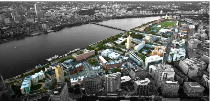
Established university campuses typically consist of a portfolio of aging buildings with a significant opportunity for energy efficiency retrofits. However, they also have a limited budget to implement upgrades. To reduce building energy use in the most cost-effective manner, university administrations therefore require a prioritization plan (e.g., MIT 2017) which offers a degree of certainty in energy cost or greenhouse gas emission reductions while also allowing them to weigh other concerns such as safety, programmatic needs, changing building uses, campus evolution, etc. The traditional energy modeling approach, which requires a large effort to build and calibrate an energy model for even a single building, in principle, can be utilized by smaller campuses to study retrofit scenarios. This option, however, is not feasible for larger campuses, which may include hundreds of buildings, such as the campus of the Massachusetts Institute of Technology (MIT) in Cambridge, MA shown in Figure 1-1.

Figure 1-1: The MIT campus in Cambridge, MA located on 168 acres (68 ha) of land that spans approximately one mile (1.6 km) along the north side of Charles River basin (image source: https://betterworld.mit.edu). This dissertation sets out to develop methods that allow universities and other institutional administrators to effectively analyze the energy saving potential of all buildings within their portfolio and support the ranking of buildings in order of energy savings potential. The remainder of this chapter further discusses the motivation for this research, presents previous efforts to analyze the energy saving potential of large university campuses, and identifies the needs and opportunities to develop new workflows that are described in the following chapters.

(16)

1.1. Large university campus characteristics

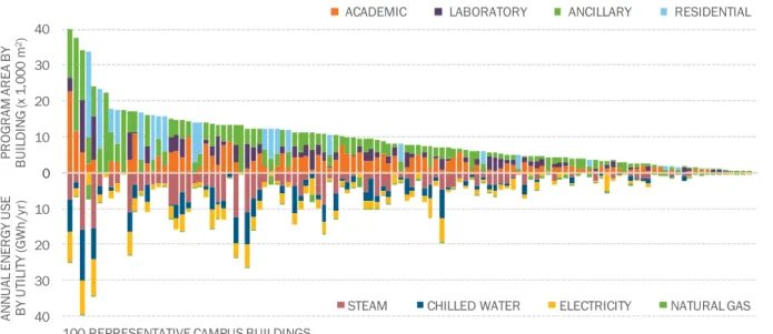
Large university campuses exhibit unique qualities: they are long-term owner-occupied, have a wide variety of programmatic uses ranging from classrooms and laboratories to student dorms, and ancillary facilities; and typically have access to current and historic energy use data for most individual buildings. For instance, Figure 1-2 illustrates the extent of available information: metered utility use and program area distributions, for a stock of one-hundred buildings that represent over 85% of MIT’s overall building portfolio of approximately 1.2 million square meters.

Figure 1-2: Illustration of information available for a stock of one hundred buildings on MIT campus, including program area distribution (left), and annual energy use distribution by utility type (right).

Time and budget constraints typically necessitate that owners of such campuses look to develop prioritization plans that phase the upgrade of their entire portfolio over several years by implementing a few efficiency measures in a few buildings at a time. Such large university campuses include high diversity use buildings that need to be studied individually, cannot be easily classified into predominant archetypes and the literature review ahead will show that traditional statistical approaches that analyze large building stocks do not offer suitable resolution to formulate cost-effective carbon emissions reduction strategies at the individual building level.

Assessment models for deeper investigation into potential savings from specific measures, in specific buildings, require information about individual building energy use data as well as most building performance related parameters. Some of these parameters such as building geometry and envelope constructions are typically known or relatively easy to determine, whereas mechanical and electrical system parameters are complicated to determine and thus have high uncertainties attached to them.

0 10 20 30 40 AN N U AL EN ER G Y U SE B Y U TI LI TY (G Wh /y r)

100 REPRESENTATIVE CAMPUS BUILDINGS

STEAM CHILLED WATER ELECTRICITY NATURAL GAS

0 10 20 30 40 PR O G R AM A R EA B Y B U IL D IN G (x 1 ,0 00 m 2)

(17)

CHAPTER 1: MOTIVATION 17 SHRESHTH NAGPAL | PH.D. DISSERTATION, 2019

1.2. Calibrated building energy models

When all the physical and operational characteristics of a building cannot be determined by available evidence because the data collection process would be too costly or building access is restricted, the calibrated model development involves inverse approximation of several inputs to reconcile the model output with observed energy use. Overall, model input parameters include the building location and climate, building geometry and envelope constructions, lighting and electrical equipment characteristics, mechanical system configuration and controls, as well as usage and operational profiles for all systems. Climate data is readily available in hourly format for many locations worldwide through the US Department of Energy (US-DOE) and other sources. Building form and envelope characteristics can typically be determined from building audits or existing design documents. The assessment of electrical and mechanical system parameters, however, takes considerable time and effort, and constitutes one of the main sources of discrepancies between simulated and measured energy use (Reddy et al. 2006).

Given several input variables are inter-dependent, the above laid out calibration process is usually over-parameterized (Coakley et al. 2015; Heo et al. 2012). For example, internal electric loads could either stem from electric lighting or other electric equipment, or high conditioning loads could result from envelope conduction or infiltration losses. Traditionally, the definition of such parameters in an energy model relies on modeler experience and judgement, manual iterations, and trial and error; making the calibrated model development process considerably time and effort intensive.

Figure 1-3: Needed alternate framework to estimate properties of unknown building characteristics that reduces the model calibration time from the traditional weeks or months of manual effort to a matter of minutes There is a need for an automated and flexible rapid-response methodology (Figure 1-3) that, based on measured energy use data and a few known performance characteristics, can estimate the properties of several unknown parameters for buildings with diverse programmatic uses, and thus generate calibrated baseline energy models with minimal manual expense.

Data

Collection DevelopmentModel SimulationsIterative

Automated Data Driven Approximation Properties of Unknown Parameters Measured Energy Use Properties of Known Parameters Analysis Time Weeks to Months Traditional Workflow Needed Alternate Analysis Time Minutes to Hours

(18)

1.3. Continuous planning framework

The development of campus-wide building energy models currently requires substantial effort and expertise for detailed geometric model building, and considerable amounts of information and time for setup and calibration of individual building models. Once developed, however, campus energy models’ use is typically limited to a single moment in time and the analysis of results is limited to evaluating static proposals. These models help university administrations to evaluate potential future scenarios for the unique set of existing conditions, and to ground aspirational greenhouse-gas emission reduction targets on technical realities. Due to the considerable effort involved, however, they are not updated regularly as retrofit programs are implemented, new buildings are added, or building use or occupancy change over time.

Campus level transformations typically stretch over decades, from retrofitting programs for buildings to façade renewal efforts. Campus conditions are also in constant flux as building uses change and student populations fluctuate. In principle, energy models, which incorporate performance parameters in extensive detail, can be easily updated by simply modifying the relevant inputs as condition change. A data-flow infrastructure, such as the one illustrated in Figure 1-4, which tracks energy use and campus developments over time to automatically update the underlying building energy models, has the potential to serve as a facility planning platform on an ongoing basis.

Figure 1-4: An example of the needed data flow infrastructure that tracks energy use and campus developments over time, automatically updates models, and allows facility planners to remotely evaluate scenarios at any time. University campuses can benefit from a framework that allows for continuous energy performance tracking and expands the point-in-time analysis capabilities of conventional energy modeling platforms. This would enable the management of building energy-use over time by automatically tracking actual performance against earlier defined targets, updating individual building energy models following the implementation of any upgrades, and evaluating future retrofit strategies. This dissertation proposes, and validates, workflows to meet this need.

Measured Energy Weather Data Model inputs Energy models deployed on a server Interactive evolutionary interface Continuously

(19)

CHAPTER 2: STATE OF THE ART 19 SHRESHTH NAGPAL | PH.D. DISSERTATION, 2019

2. State of the Art

Large university campuses typically rely on spreadsheet tools (e.g., Brown 2012; Bricca et al. 2017; Escobedo et al. 2014), or on-site surveys [e.g., Chung et al. 2014; Vasquez et al. 2015) to estimate the current energy use for individual buildings. Other universities have employed cluster analysis to determine load features of different building groups (Guan et al. 2016), normalized energy use based on site weather information, and developed reduced order models defined by only a few influential input variables (Heidarinejad et al. 2017), to provide data for evaluating potential strategies. Finally, recent studies have presented web-based platforms (Chen et al. 2017), and software (Robinson et al. 2009) designed to allow users to quickly set up and run urban energy models with case studies (e.g., Coccolo et al. 2015) that analyze energy demand of buildings and evaluate alternate scenarios.

Figure 2-1: University campuses across the world that have been researching the development of building energy models for their campuses to understand existing conditions, and plan for future scenarios.

All of the above models developed for different universities highlighted in Figure 2-1 are based on the premise that the complex nature of building energy use renders the calibration of numerous building energy models time and effort intensive, and do not fully capture the unique architectural features, programmatic requirements, or the electrical and mechanical systems configurations of individual campus buildings. As a result, without access to individual building performance characteristics, these cluster or archetype level urban energy models are able to provide general guidance across multiple buildings but are unable to assess future scenarios for individual buildings. This chapter presents existing work in the field of building energy analysis for large building stocks, identifies and discusses recent developments in computational techniques that are significant for this research, and illustrates the gaps that this dissertation attempts to close.

(20)

2.1. Urban building energy modeling

Over the past few years, a genre of urban building energy models or UBEM (Reinhart & Cerezo 2015) has been developed. These bottom-up engineering methods apply building energy modeling concepts to a large number of buildings at a neighborhood, or even a city scale (Figure 2-2) (Sokol et al. 2017). UBEMs divide a given building stock into archetypes, and assign the same construction standards, usage patterns, and mechanical and electrical system parameters to all buildings within an archetype. Once calibrated to measured energy use of a subset of buildings, UBEMs have been shown to successfully project total energy use of residential neighborhoods (Cerezo et al. 2016).

Figure 2-2: 3D view of the urban building energy model for the city of Cambridge (Sokol et al. 2017). The outlined building subset was used to train models that could then effectively simulate all neighborhoods.

When upgrades are to be implemented across a large number of buildings, Bayesian calibration based UBEMs have been shown to simulate the diversity of monthly energy uses of buildings within an archetype and predict neighborhood level savings (Howard et al. 2012). Such UBEMs have been utilized by municipalities for developing suitable energy policy measures and to assess broad scope greenhouse gas emission reductions for residential neighborhoods (Cerezo et al. 2015).

Large university campuses, in contrast to residential neighborhoods, include buildings with high diversity uses which cannot be easily classified into a single predominant archetype. For projects where each building needs to be evaluated individually, UBEM approaches need to be complemented with calibrated individual building models to formulate effective carbon reduction strategies.

training set buildings

(21)

CHAPTER 2: STATE OF THE ART 21 SHRESHTH NAGPAL | PH.D. DISSERTATION, 2019

2.2. Automated calibration techniques

Automatic building level energy model calibration, with the goal of computationally estimating the unknown characteristics of a building based on some known building properties and measured energy use information, has been a focus of research in recent years (e.g. Fabrizio & Monetti 2015; Robertson et al. 2013). Most of these techniques utilize an optimization function (Figure 2-3) to reduce the difference between measured and simulated data by iteratively adjusting the values of unknown parameters. Studies have proposed employing brute-force sampling (New et al. 2012), graphical pattern recognition (Sun et al. 2016), and global optimization algorithms (Lee & Claridge 2002) to iteratively adjust the values of unknown parameters until the difference between measured and simulated data is minimized. These techniques essentially replace the manual trial-and-error based iterative parameter adjustment by mathematically informing the input assumptions for a simulation run based on results from earlier iterations.

Figure 2-3: Most auto-calibration techniques require numerous energy simulations that iteratively adjust values of unknown parameters until the difference between measured and simulated energy use is within desired range. While these techniques can significantly reduce the high time and cost expense associated with experienced auditors and modelers working through the calibration process, they still result in a considerable computational expense required to generate and run hundreds of thousands of energy simulations, making these techniques inaccessible in most scenarios.

This computational cost can, in principle, be significantly reduced if these auto-calibration methods, which currently rely on detailed engineering models to simulate each iteration, could instead incorporate data-driven approximation techniques that employ statistical models. In combination with established model generation techniques from UBEM, these hybrid methods could potentially develop calibrated models considerably faster than traditional approaches.

List of Unknown Parameters Building Energy Simulation Measured Energy Use Calibrated Model Properties of Known Parameters New Sample Parameter Combination Error in Range? Modeled Energy Use Y N Iterative Evolutionary Algorithm

(22)

2.3. Surrogate modeling strategies

Surrogate models constitute a class of machine learning algorithms designed to make computation faster and enable more productive exploration and optimization of design variables (Forrester et al. 2008; Mueller 2014). These algorithms attempt to create mathematical models of the physical behavior of systems based only on available data, using statistical techniques such as regression. Figure 2-4 illustrates how a few computer-generated samples are created and then fit to an approximation model, which can then directly generate new representative data samples without the need for computationally expensive engineering simulations. Once trained using a small simulation-generated sample set, the surrogate models can provide instant feedback associated with changing individual building characteristics and can vastly reduce the computation time required by optimization routines to find the best solutions.

Figure 2-4: A surrogate regression model is trained to replicate a physical behavior (left) based on a collection of pre-computed data points (middle). With enough training data (right), the resulting model can be used to predict performance for other points in the design space with some degree of error (Redrawn, Mueller 2014). There are several approximation algorithms that are designed to fit detailed simulation results to a statistical function, a few of which have been studied for their effectiveness in reducing the computational expense associated with detailed building energy simulations (Aijazi & Glicksman 2016; Tsanas & Xifara 2012). Utilizing these trained surrogate models, an optimization algorithm (e.g. Brown 2016, Tseranidis et al. 2016) can be used to search for the combination of unknown parameters that results in the highest performance score. While both gradient-based and stochastic optimization algorithms can be used with surrogate models, the typical optimization process starts with random samples in the design space, and then use stochastic operators to direct the process of finding the highest score. While employing surrogate models in lieu of detailed engineering models can, in principle, significantly expedite this process, it has not been researched specifically for incorporation in auto-calibration routines for developing building energy models.

PE R FO R M AN C E SC O R E

COMBINATION OF INPUT VARIABLES

Actual behavior Training data Surrogate model Actual behavior Actual behavior Training data Surrogate model

(23)

CHAPTER 3: CHALLENGES AND OPPORTUNITIES 23 SHRESHTH NAGPAL | PH.D. DISSERTATION, 2019

3. Challenges and Opportunities

The previous two chapters present the significant work that has been done in the field of building energy modeling, especially as it relates to evaluations of large building stocks, and highlight the critical areas that need to be addressed before the current tools can be utilized by university campuses to plan for future energy scenarios. Large campuses include several diverse-use buildings that need to be evaluated individually to manage their greenhouse gas emissions targets. These buildings cannot be easily classified into programmatic archetypes rendering the traditional urban building energy modeling approaches insufficient. In addition, the complex nature of institutional building characteristics makes the development of calibrated energy models for individual buildings prohibitively time and effort intensive. Finally, even when substantial time and effort is invested, the models are typically designed to be only used once, to evaluate static proposals relevant for the unique set of existing conditions, at a single point in time.

3.1. Research goal

To address some of the above limitations, the goal of this research is to develop new workflows for the generation of calibrated campus energy models, that are designed to evaluate future building level upgrades, present their consequences to decision makers on an ongoing basis, and enable administrators to manage their building related greenhouse gas emissions over time.

3.2. Hypotheses

This research is based on the premise that it is important and possible to generate such models, and is founded on the following hypotheses which are revisited in the concluding chapter:

 Feasibility: surrogate modeling techniques can considerably reduce the required time and effort to generate calibrated bottom-up energy models for large university campuses that enable building-by-building evaluation of potential retrofits and future energy scenarios.

 Reliability: the resulting auto-calibrated energy models can identify the areas of maximum potential savings within reasonable limits of uncertainty and allow campus owners to systematically study only the high priority areas in further detail for more accurate assessments.



Significance: bottom-up campus energy models yield accurate simulation results for building level assessments and have the potential to evolve continuously over time allowing them to be utilized as continuous planning tools as university campuses implement their retrofit plans.

(24)

3.3. Organization of dissertation

This dissertation is divided into three parts: Introduction, Workflows, and Conclusions.

Part I: Introduction, includes the first three chapters, and addresses the need for study and background work for research questions considered in this dissertation.

Chapter 1: Motivation, presents the motivation for this research, critiques existing methods for their strengths and limitations, and identifies the needs to develop new workflows.

Chapter 2: State of the Art, presents an overview of existing work, discusses developments in relevant computational techniques, and identifies the areas for further research.

Chapter 3: Challenges and Opportunities, discusses the challenges with current tools to illustrate the opportunities for further research, and lays out specific objectives of this research.

Part II: Workflows, is broken down into four chapters, each of which will describe a proposed new workflow for a different development stage of university campus energy models.

Chapter 4: Modeling Approach, assesses the strengths and limitations of two recent urban modeling methodologies and suggests best practice procedures for large university campuses. Chapter 5: Automated Calibration, evaluates a methodology to develop baseline campus models by employing surrogate models for rapid estimation of unknown building parameters.

Chapter 6: Energy Supply Systems, presents a planning tool that translates simulation results from calibrated models for building energy use to associated greenhouse gas emissions.

Chapter 7: Continuous Planning Framework, proposes an energy performance planning system that enables campuses to assess and manage building related greenhouse gas emissions over time. Part III: Conclusions, discusses how these workflows could be employed in practice and concludes

the dissertation with a summary of contributions in the final two chapters.

Chapter 8: Summary and Discussion, summarizes the specific contributions of this dissertation and discusses the possibilities of integrating these workflows as a single unified approach.

Chapter 9: Research Outlook, discusses the potential impact of this thesis, envisioned applications, and important directions for future research.

(25)

(26)

(27)

II. WORKFLOWS

This section first presents, in Chapter 4, two previously developed calibrated energy models for the MIT campus – one based on a spreadsheet approach with select BEMs in the background, and the second an archetype-based UBEM – and establishes the minimum model requirements needed to develop campus retrofit plans for assessment of upgrade strategies for individual buildings.

To work towards an ideal campus model that meets the above requirements, while significantly reducing the computational cost of developing hundreds of calibrated building energy models, Chapter 5 proposes a hybrid auto-calibration methodology that combines model generation techniques from UBEM with rapid-response data-driven approximation techniques.

Chapter 6 presents a planning tool developed to evaluate district energy system configurations in combination with campus building energy models. This tool identifies opportunities to reduce campus greenhouse gas emissions from an optimal selection of campus electricity and thermal energy supply systems, including the incorporation of renewable energy sources.

Finally in this section, Chapter 7 presents a framework to expand the point-in-time analysis capabilities of conventional urban energy modeling platforms and presents a tool for the development and implementation of campus-level continuous energy-performance tracking and planning system. The system archives historic data, enables exploration of potential upgrade scenarios, and allows for the documentation of energy retrofits to individual buildings.

(28)

(29)

1_{A version of this chapter has been published: S. Nagpal, C. Reinhart, A comparison of two modeling approaches for} establishing and implementing energy use reduction targets for a university campus, Energy and Buildings, 2018.

4. Modeling Approach

1

The Office of Sustainability at MIT, in response to the City of Cambridge’s Net Zero Action Plan (2015), recently completed a feasibility study for potential upgrades to existing campus buildings (MIT 2017). To work towards the ideal urban model for a campus that provides the fidelity of information that a collection of individual calibrated building energy models would yield while requiring the same effort as to build an urban building energy model, two models were recently developed for the campus of the Massachusetts Institute of Technology. The first approach utilizes a combination of statistical techniques that attribute energy use to the primary programmatic uses on campus before evaluating the effect of energy efficiency measures for those specific program types; and the second (Figure 4-1) bottom-up engineering approach develops an urban building energy model for the campus designed to forecast the impact of building-by-building retrofit scenarios.

Figure 4-1: Graphic rendering of the urban building energy model for MIT campus showing distribution of programmatic archetypes. This is one of the two models developed to study the feasibility of potential energy efficiency upgrades to existing buildings in response to the City of Cambridge’s Net Zero Action Plan (2015). This chapter reviews these two models with regards to their setup and calibration effort, ability to model current individual building energy use vis-à-vis measured data as well as predicted savings from implementing a variety of retrofitting measures. Sections in this chapter will describe the two approaches in detail with regards to the model inputs and the underlying development procedures, and compare and contrast the results from these two models for baseline conditions as well as potential retrofit scenarios at campus and individual building levels. The objectives are to identify both models’ strengths and weaknesses and to suggest best practice procedures for administrators of other campuses interested in undergoing a similar exercise.

(30)

4.1. Studied workflows

Each building on the MIT campus is broadly classified as academic, laboratory, ancillary or residential, based on the predominant programmatic use. In addition, detailed floor area compositions with fifteen functional uses have also been compiled for most buildings. As an example, Table 4-1 presents a sample of the available information for three representative campus buildings.

Table 4-1: Level of available information: known program area distribution and utility consumption for three representative campus buildings.

Building Type Laboratory Academic Residential

Total Area (m2₎ _30,233 _8,851 _14,044 Area Distribution (%) Academic Spaces 1 Offices 11% 24% - 2 General Use I 2% 2% 12% 3 General Use II - - - 4 Classrooms - 27% - 5 Study - - - Laboratory Spaces 6 Lab Type I 43% - - 7 Lab Type II - - - 8 Special Use 3% - - 9 Athletic - - - Ancillary Spaces 10 Circulation 19% 24% 26% 11 Mechanical 17% 19% 3% 12 Garage - - - 13 Support 3% 1% - 14 Services 2% 3% 6% Residential Spaces 15 Dormitories - - 53%

Utility use (GWh/yr)

Steam/Natural Gas 19.44 2.53 3.15

Chilled Water 8.04 0.93 -

Electricity 9.97 0.90 2.43

Figure 4-2 presents this program area distribution across the campus as a tree-map, where colors represent four predominant space categories that are broken down by detailed program uses within each category. The maps illustrate that ancillary uses such as circulation, support and mechanical spaces occupy almost 35% of overall campus floor area, followed by academic spaces at about 30%. Labs occupy less than 20% and residential spaces constitute 15% of the floor area.

(31)

CHAPTER 4: MODELING APPROACH 31 SHRESHTH NAGPAL | PH.D. DISSERTATION, 2019

Figure 4-2: Campus floor area distribution by programmatic use.

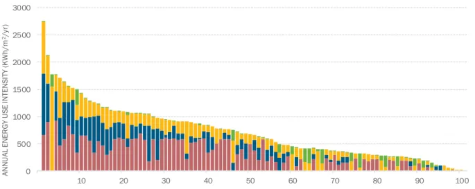
The annual energy use data for all buildings, broken down by three utility end-uses, is also available for each building. Most campus buildings are served by the campus central co-generation plant and monitored via building utility meters for steam and electricity consumption. The academic and laboratory buildings are served by campus chilled water for space cooling which is also metered at the building level. Most residential buildings, in contrast, incorporate individual electric packaged terminal air conditioners for dormitories, and the energy associated with space cooling is included in the metered electricity consumption. Figure 4-3 illustrates this information for most MIT campus buildings arranged in order of decreasing energy use intensities, where each column represents an individual building, with known annual utility use breakdown plotted on the y-axes.

Figure 4-3: Information available for 100 MIT main campus buildings for 2016 (Source: MIT Office of Sustainability). SPECIAL USE ATHLETIC LAB TYPE I SUPPORT LAB TYPE II SERVICES MECHANICAL CIRCULATION DORMITORIES OFFICES GENERAL

USE I GENERALUSE II

CLASSROOMS STUDY 0 5 10 15 20 25 30 35 40 45 50 10 20 30 40 50 60 70 80 90 100 PR O G R AM A R EA B Y B U IL D IN G (x 1 ,0 00 m 2)

REPRESENTATIVE CAMPUS BUILDING

ACADEMIC LABORATORY ANCILLARY RESIDENTIAL

0 500 1000 1500 2000 2500 3000 10 20 30 40 50 60 70 80 90 100 AN N U AL EN ER G Y U SE IN TEN SI TY (K W h/m 2/y r)

(32)

4.1.1. Model 1: Spreadsheet Approach

This method, developed for MIT by the environmental design consulting firm Atelier Ten, utilizes a simple statistical technique to calculate energy use intensities (EUI) that can be attributed to the 15 programmatic uses from Table 1. The approach assumes that the EUI for each program use (EUIPU)

depends primarily on the internal load and operating parameters, and is not significantly affected by variations in envelope configuration, age of the building, or other design parameters. In other words, for the purpose of this model, the 15 EUIPU are assumed identical across all campus buildings.

The total annual campus energy use, EC, can then be expressed as a linear function of the floor area of the different programmatic uses within each building, APU (Building), and the average energy use

intensity for each programmatic use and energy end use, EUIPU (End Use). For the 100 campus

buildings, 15 different programmatic uses and three energy end uses (electricity, steam and chilled water) and the model can be expressed as:

𝐸𝐶 = ∑ 𝐸𝐵 , 𝑎𝑛𝑑 100 𝐵=1 𝐸𝐵 = ∑ 𝐴𝑃𝑈(𝐵𝑢𝑖𝑙𝑑𝑖𝑛𝑔) 15 𝑃𝑈=1 × ∑ 𝐸𝑈𝐼𝑃𝑈(𝐸𝑛𝑑 𝑈𝑠𝑒) 3 𝑈=1 … (1) where,

𝐸𝐶: known total annual energy use for studied building stock 𝐸𝐵: known annual energy of a specific building

𝐵: 1 of 100 studied campus buildings 𝑃: 1 of 15 campus programmatic uses 𝑈: 1 of 3 campus utility end-uses

𝐴𝑃𝑈: known floor area of specific program type in a specific building

𝐸𝑈𝐼𝑃𝑈: campus average energy use intensity for a specific end-use and program type

Given that the annual utility consumption for 3 end-uses for chilled water, steam/natural gas, and electricity as well as floor areas of 15 program types were known for all campus buildings, all 45 (3x15) EUIPU (Energy Use) values could be regressed from Equation 1. The resulting values are listed

(33)

Table 4-2: Regressed energy use intensity for 15 campus program uses.

# Program Use Energy Use Intensity (EUIPU - kWh/m2-yr)

Chilled water Steam /Natural Gas Electricity Total

Academic Spaces 1 Offices 173 231 290 694 2 General Use I 66 213 83 362 3 General Use II 132 201 83 416 4 Classrooms 115 204 83 402 5 Study 99 207 83 389 Laboratory Spaces 6 Lab Type I 123 259 103 486 7 Lab Type II 444 878 432 1,755 8 Special Use 1,728 3,100 2,028 6,856 9 Athletic 432 854 420 1,706 Ancillary Spaces 10 Circulation 202 357 145 704 11 Mechanical 230 352 145 727 12 Garage 4 8 4 16 13 Support 49 96 50 195 14 Services 16 222 83 321 Residential Spaces 15 Dormitories 12 144 87 243

As explained in the introduction, the primary purpose of this campus energy model is to provide a mechanism for predicting the change in energy use for future retrofit and evolution scenarios. However, the data from Table 4-2 can only be used to calculate energy use impact of scenarios if a known program type is added or converted into another known program type. In addition, this spreadsheet model can only extrapolate from current performance, and cannot evaluate energy savings associated with future high-performance retrofits.

To expand the capabilities of the spreadsheet model to evaluate potential future scenarios, simple transient block energy models were developed for each of the four predominant space categories using the eQuest interface for DOE2.2 (Hirsch, 1998) simulation engine. Figure 4-4 illustrates these block energy models that consist of a five-floor, five-zone per floor, 10,000 m2_{thermal model with a}

(34)

Table 4-3 presents the envelope, internal load and mechanical system parameters that were manually adjusted based on a combination of modeler experience and campus knowledge, and numerous iterative simulations of the baseline eQuest models until the results fit the energy use intensities in Table 4-2.

Figure 4-4: Graphic representation of eQuest block energy model.

Table 4-3: Key input parameters for block-energy models.

Input parameters Residential Spaces Academic Spaces Ancillary Spaces Laboratory Spaces

Envelope Characteristics

Wall construction U:0.70 W/m2_K _{U:0.40 W/m}2_K _{U:0.70 W/m}2_K _{U:0.40 W/m}2_K Roof construction U:0.60 W/m2_K _{U:0.35 W/m}2_K _{U:0.60 W/m}2_K _{U:0.35 W/m}2_K Fenestration type U:5.50 W/m2_K _{U:2.50 W/m}2_K _{U:5.50 W/m}2_K _{U:2.50 W/m}2_K Glazing ratios 40% of wall area 40% of wall area 40% of wall area 40% of wall area

Internal Loads Occupant density 0.5 pp/m2 _{0.2 pp/m}2 _{0.5 pp/m}2 _{2.0 pp/m}2 Equipment power 10 W/m2 _{35 W/m}2 _{50 W/m}2 _{150 W/m}2 Lighting power 10 W/m2 _{12 W/m}2 _{12 W/m}2 _{12 W/m}2 Mechanical systems Heating set-point 23.0 o_C _22.0o_C _22.0o_C _22.0o_C Cooling set-point 24.0 o_C _24.0o_C _24.0o_C _24.0o_C

Zone terminal units - Hot water reheat Hot water reheat Hot water reheat

Ventilation flowrate - 140 ls-1_/person _- _{12 ACH}

Fan system power - 2.5 W/ls-1 _{2.5 W/ls}-1 _{4.0 W/ls}-1

Pump power - 220 W/ls-1 _- _{220 W/ls}-1

Heating source Campus steam Campus steam Campus steam Campus steam

Cooling source Electric DX, COP 3.0 Campus chilled water Campus chilled water Campus chilled water 45m 45m 8m CORE ZONE

SOUTH PERIMETER ZONE 5-FLOOR, 10,000m2

5-ZONE PER FLOOR eQUEST ENERGY MODEL

EA ST P ER IM ET ER Z O N E WES T PE R IM ET ER Z O N E

(35)

The resulting “calibrated” block energy models were employed to simulate the energy impact of potential efficiency upgrades. To extrapolate the projected energy savings from these models back to the overall campus model, the energy savings projected by these models for any retrofit scenario were translated into percentage reduction factors, 𝑅𝐹_𝑆𝑈, for cooling, heating, and electricity end-uses for each space category. The post-retrofit energy use for each building could then be calculated by multiplying the reduction factors for each space category within that building, with the pre-retrofit energy use. This potential energy savings estimate was then expressed via the following simple equation: 𝐸𝐶𝑅 = ∑ 𝐸𝐵𝑅, 100 𝐵=1 𝑎𝑛𝑑 𝐸𝐵𝑅 = ∑ 𝐴𝐵𝑆 4 𝑆=1 × ∑(𝐸𝑈𝐼𝑆𝑈× 𝑅𝐹𝑆𝑈) 3 𝑈=1 … (2) where,

𝐸𝐶𝑅: post-retrofit campus total annual energy use

𝐸𝐵𝑅: post-retrofit annual energy use for a specific building 𝐵: 1 of 100 studied campus buildings

𝑆: 1 of 4 campus space categories 𝑈: 1 of 3 campus energy end-uses

𝐴𝐵𝑆: floor area of specific space category in a specific building

𝐸𝑈𝐼𝑆𝑈: pre-retrofit energy use intensity for a specific end-use, for a specific space category 𝑅𝐹𝑆𝑈: reduction factor associated with the studied retrofit measure – for a specific space

category, for a specific energy use, based on percentage savings simulated by block energy model for that space category; set at 1 for any building that already

incorporates the studied measure 4.1.2. Model 2: UBEM approach

The second campus model is a bottom-up engineering or urban building energy model developed at the Sustainable Design Lab at MIT. It is based on the assumption that building energy use depends on more than floor areas of programmatic use type and that variations in envelope configuration, lighting and mechanical systems, and occupant behavior can result in considerably different energy use profiles for individual buildings even if their predominant programmatic use is the same.

(36)

This means that a dynamic energy model has to be individually fitted for each building on campus using the simulation input parameters listed in Table 4-4. The resulting model cannot be expressed as a set of simple equations, but as a function of multiple input parameters, 𝜃_𝐵𝑛, specific to each individual building, B: 𝐸𝐶 = ∑ 𝐸𝐵, 𝑎𝑛𝑑 100 𝐵=1 𝐸𝐵= 𝑓(𝐶, 𝜃𝐵1, 𝜃𝐵2, … 𝜃𝐵𝑛) … (3) where,

𝐸𝐶: total campus annual energy use

𝐸𝐵: modeled energy use of a specific building, calibrated to measured data 𝐵: one of 100 campus buildings

𝑓: systems of equations employed by the building energy simulation engine 𝐶: typical meteorological year climate data file for campus location

𝜃𝐵𝑛: one of multiple model input parameters for each individual building (see Table 4)

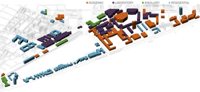
In addition to the detailed program type distribution utilized for the spreadsheet model, the UBEM requires the combination of several datasets including climate data, building geometry, construction standards, usage schedules, and loads and systems parameters to simulate individual building energy use. A campus-wide Geographic Information System (GIS) database was utilized to automatically generate extruded massing models of the campus. Additional envelope data, which consisted of floor heights, fenestration configuration, window opening ratios, and construction assemblies, was based on architectural drawings or on visual inspection where drawings were not available. The building stock was then abstracted into four predominant programmatic archetypes that represent a group of buildings with similar non-geometric properties. Figure 4-5 presents a graphic rendering of the campus energy model showing distribution of academic, laboratory, ancillary and residential archetypes. The UBEM is developed for EnergyPlus v.8.4 whole building energy simulation program using the UMI components for Grasshopper, a plugin to the CAD environment Rhinoceros3D (McNeel, 2015). Figure 4-6 presents a tree-map for campus floor area distribution, where the colors represent four predominant building types, broken down by individual building areas within each category. The maps suggest that laboratory buildings occupy 38%, academic buildings account for 33% and residential and ancillary buildings constitute 28% and 5% of the total campus floor area, respectively.

(37)

Figure 4-5: Graphic rendering of UBEM showing distribution of programmatic archetype.

Figure 4-6: Campus floor area distribution by building type.

Input templates were created for each of these archetypes and assigned, one per building, across the campus. Non-geometric performance properties, such as occupant densities, lighting and miscellaneous equipment power, and usage schedules were estimated based on building program uses, and adjusted within defined ranges as part of the process to calibrate individual building models to measured energy use.

Mechanical systems were defined to translate building loads to campus steam and chilled water consumption by applying an overall coefficient of performance of 1.0 to space heating and space cooling energy. These model input parameters, and their defined ranges for different programmatic archetypes, are summarized in Table 4-4.

0 5 10 15 20 25 30 35 40 45 50 10 20 30 40 50 60 70 80 90 100 PR O G R AM A R EA B Y B U IL D IN G (x 1 ,0 00 m 2)

LABORATORY

38% ACADEMIC33% RESIDENTIAL28%

ANCILLARY 5%

(38)

Table 4-4: Summary of key UBEM input parameter ranges.

Input parameters (θn) Residential Buildings Academic Buildings Ancillary Buildings Laboratory Buildings

Envelope Characteristics

Building Geometry GIS dataset GIS dataset GIS dataset GIS dataset

Glazing ratios 15% - 50% 15% - 50% 15% - 50% 15% - 50%

Wall construction U:0.71–0.38 U:0.71–0.38 U:0.71–0.38 U:0.71–0.38

Roof construction U:0.62–0.15 U:0.62–0.15 U:0.62–0.15 U:0.62–0.15

Window Conductance U:5.78–1.96 U:5.78–1.96 U:5.78–1.96 U:5.78–1.96

Glazing SHGC 0.82–0.69 0.82–0.69 0.82–0.69 0.82–0.69

Internal Load Ranges

Occupants (pp/m2₎ _{0.5 pp/m}2 _{0.1 – 0.3 pp/m}2 _{0.5 pp/m}2 _{1.5 – 2.5 pp/m}2

Equipment (W/m2₎ _{8 – 10 W/m}2 _{25 – 55 W/m}2 _{50 W/m}2 _{60 - 200 W/m}2

Lighting (W/m2₎ _{8 – 10 W/m}2 _{12 W/m}2 _{12 W/m}2 _{12 W/m}2

Mechanical systems

Heat set-point (o_C) _{22.0 – 24.0}o_C _{21.5 – 22.5}o_C _22.0o_C _{21.5 – 22.5}o_C Cool set-point (o_C) _{22.0 – 25.0}o_C _{22.0 – 22.5}o_C _n/a _{21.5 – 22.5}o_C

Ventilation flowrate - 120 - 180 ls-1_/p _- _{6 - 12 ACH}

Heating source Campus steam Campus steam Campus steam Campus steam

Cooling source Electric DX, COP 3.0 Chilled water n/a Chilled water The simulation of different retrofit strategies with this model simply requires the modification of inputs from existing parameters to potential scenarios. The potential campus-wide energy savings could then be simulated by the following model:

𝐸𝐶𝑅 = ∑ 𝐸𝐵𝑅, 𝑎𝑛𝑑 100

𝐵=1

𝐸𝐵𝑅 = 𝑓(𝐶, 𝜃𝐵𝑅1, 𝜃𝐵𝑅2, … 𝜃𝐵𝑅𝑛) … (3)

where,

𝐸𝐶𝑅: post-retrofit campus total annual energy use

𝐸𝐵𝑅: post-retrofit annual energy use for a specific building 𝐵: one of 100 studied campus buildings

𝑓: systems of equations employed by the building energy simulation engine 𝐶: typical meteorological year climate data file for campus location

𝜃𝐵𝑅𝑛: one of multiple model input parameters associated with the studied retrofit measure for a specific building; set same as 𝜃_𝐵𝑛 if not affected by the measure.

(39)

CHAPTER 4: MODELING APPROACH 39 SHRESHTH NAGPAL | PH.D. DISSERTATION, 2019 4.1.3. Modes of Comparison

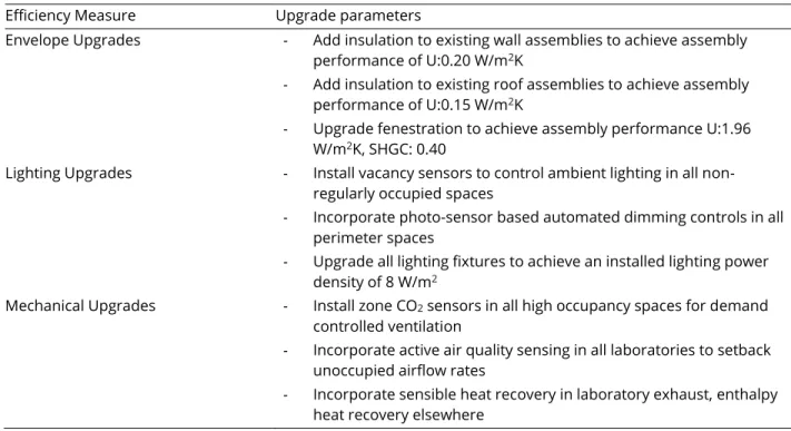
While the procedures for setting up the spreadsheet and UBEM models vary considerably, the purpose of both models is to simulate future scenarios to predict potential changes in campus and building-by-building energy use. To better understand the differences between the two models, and to assess their applicability in different situations, the results from both models are compared for various scenarios. First, the baseline results that represent existing conditions are compared to assess the calibration accuracy of each model at the overall campus scale, as well as at an individual building level. The next analysis assumes that all upgrades listed in Table 4-5 are implemented in the entire building stock across all programmatic archetypes on campus and presents a high-level forecast of potential future energy use to help inform campus level planning issues.

Table 4-5: Summary of pre-programmed parameters considered for retrofit scenarios.

Efficiency Measure Upgrade parameters

Envelope Upgrades - Add insulation to existing wall assemblies to achieve assembly performance of U:0.20 W/m2_K

- Add insulation to existing roof assemblies to achieve assembly performance of U:0.15 W/m2_K

- Upgrade fenestration to achieve assembly performance U:1.96 W/m2_{K, SHGC: 0.40}

Lighting Upgrades - Install vacancy sensors to control ambient lighting in all non-regularly occupied spaces

- Incorporate photo-sensor based automated dimming controls in all perimeter spaces

- Upgrade all lighting fixtures to achieve an installed lighting power density of 8 W/m2

Mechanical Upgrades - Install zone CO2 sensors in all high occupancy spaces for demand controlled ventilation

- Incorporate active air quality sensing in all laboratories to setback unoccupied airflow rates

- Incorporate sensible heat recovery in laboratory exhaust, enthalpy heat recovery elsewhere

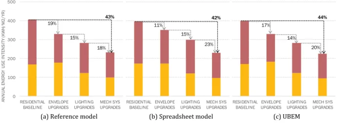
Finally, three buildings – one each from laboratory, academic and residential categories – were picked to compare results at individual building scale. The retrofit scenarios are simulated for each building, and the results from both models are compared against projections from separately developed reference calibrated BEMs. These reference models, graphically represented in Figure 4-7, incorporate building massing characteristics, floor-by-floor spatial programmatic distribution, as well as detailed operational, electrical, and mechanical system parameters for each building.

(40)

(a) Laboratory building (b) Academic building (c) Residential building Figure 4-7: Graphic representation of reference whole building energy models showing program distribution. As discussed earlier, the models used in the spreadsheet approach account for distribution of various program types within each building but assume campus average performance parameters for each program type, while the UBEMs which incorporate building specific performance parameters but assume a single set of operational characteristics for all spaces within the building. The aim of this last study is to assess the effectiveness of the two studied campus modeling approaches, which simplify individual building models in distinct ways, against a reference BEM, which incorporates all details, for various upgrade scenarios.

4.2. Results

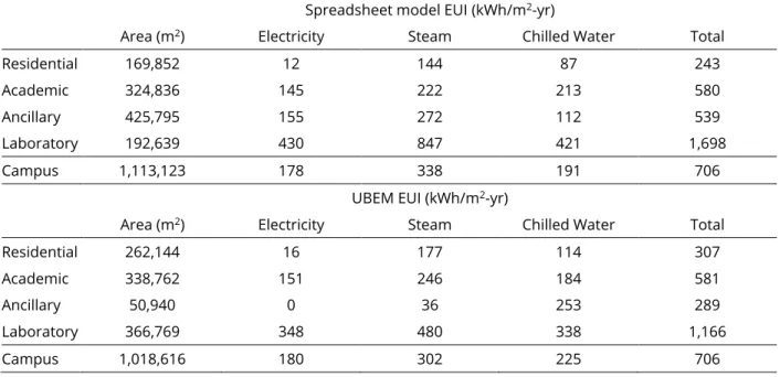
In its baseline state, the spreadsheet model statistically represents overall campus energy use without relying on building level energy analysis. Table 4-6 lists the baseline energy use intensities calculated by the spreadsheet model for the four predominant space categories that were earlier presented in Table 4-2. The UBEM, on the other hand, explicitly simulates each building individually to predict energy use based on detailed input parameters. To enable comparison between the results from two models, Table 4-6 also organizes simulation results for the UBEM baseline by campus-average energy use intensities for the four predominant building types.

4.2.1. Campus level baseline

The results in Table 4-6 show that while the overall campus areas are within 10% of each other between the two models, the area distribution by program type differs considerably. This is because the first model is a statistical representation of existing conditions where multiple programmatic uses are distributed within each building, whereas the UBEM calculates building area based on GIS footprint data and defined number of floors, and assigns each building with a single programmatic archetype based on the predominant use in that building.

0 5 10 15 20 25 30 35 40 45 50 10 20 30 40 50 60 70 80 90 100 PR O G R AM A R EA B Y B U IL D IN G (x 1 ,0 00 m 2)

(41)

Table 4-6: Baseline energy use intensities for predominant space categories: spreadsheet and UBEM approach. Spreadsheet model EUI (kWh/m2_-yr)

Area (m2₎ _Electricity _Steam _{Chilled Water} _Total

Residential 169,852 12 144 87 243

Academic 324,836 145 222 213 580

Ancillary 425,795 155 272 112 539

Laboratory 192,639 430 847 421 1,698

Campus 1,113,123 178 338 191 706

UBEM EUI (kWh/m2_-yr)

Area (m2₎ _Electricity _Steam _{Chilled Water} _Total

Residential 262,144 16 177 114 307

Academic 338,762 151 246 184 581

Ancillary 50,940 0 36 253 289

Laboratory 366,769 348 480 338 1,166

Campus 1,018,616 180 302 225 706

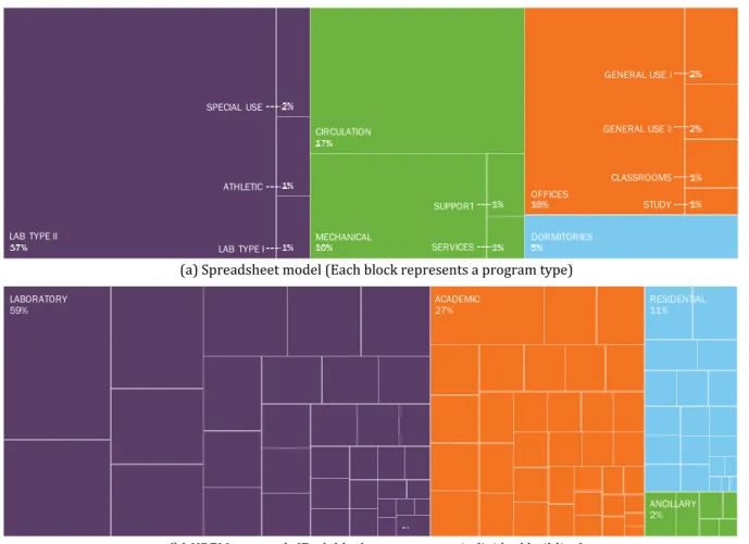
The overall campus energy use intensity results, however, match closely between the two models illustrating that both models are successfully calibrated to measured energy use at the campus scale. Figure 4-8 compares the energy use distribution between the two models through tree-maps where the colors represent four predominant program types. A comparison of these maps for baseline conditions show that lab spaces in the spreadsheet model (a) result in just under 40% of the campus energy, whereas lab buildings in the UBEM (b) account for almost 60% of total campus energy use. This difference can be attributed primarily to ancillary uses, such as lab support spaces, that account for just under 30% of the campus energy in the spreadsheet model, but are included within other building types in the UBEM. The buildings that are classified as ancillary in the UBEM only constitute 2% of total energy.

4.2.2. Individual building baselines

Figure 4-9 compares measured against simulated annual energy use for individual buildings according to both campus models. The coefficients of determination for the spreadsheet and UBEM are 0.85 and 0.96, respectively, while the number of building whose measured and simulated energy uses diverge by more than 20% are 57 for the spreadsheet and 25 for the UBEM model. For the spreadsheet models, differences are smallest for lab buildings whose energy use is driven primarily by functional requirements. In contrast, the UBEM approach performs best for envelope dominated buildings.

(42)

(a) Spreadsheet model (Each block represents a program type)

(b) UBEM approach (Each block represents an individual building)

Figure 4-8: Comparison of campus energy use distribution by program type between two models.

(a) Spreadsheet model (b) UBEM approach

Figure 4-9: Correlation of measured vs modeled energy use for individual buildings. SPECIAL USE ATHLETIC LAB TYPE I SUPPORT LAB TYPE II SERVICES MECHANICAL CIRCULATION DORMITORIES OFFICES GENERAL USE I GENERAL USE II CLASSROOMS STUDY LABORATORY 59% ACADEMIC27% RESIDENTIAL11% ANCILLARY 2% 0 5 10 15 20 25 30 35 40 45 50 10 20 30 40 50 60 70 80 90 100 PR O G R AM A R EA B Y B U IL D IN G (x 1 ,0 00 m 2)

5 10 15 20 25 - 5 10 15 20 25 R EG R ES SED EN ER G Y U SE (M W h/ yr )

MEASURED ENERGY USE (MWh/yr)

5 10 15 20 25 - 5 10 15 20 25 SI M U LA TED EN ER G Y IU SE (M W h/y r)

(43)

CHAPTER 4: MODELING APPROACH 43 SHRESHTH NAGPAL | PH.D. DISSERTATION, 2019 4.2.3. Campus level upgrades

To calculate the energy impact of identified lighting, envelope, and mechanical system retrofits listed in Table 4-5, the spreadsheet model employs block energy models for each predominant space category discussed earlier. The simulation output from these block energy models for each of these upgrade scenarios is translated into reduction factors for cooling, heating, and electricity end-uses. The resulting reduction factors for each program type are presented in Table 4-7.

Table 4-7: Retrofit energy reduction factors by energy end-use.

Upgrades Envelope Upgrades Lighting System Upgrades Mechanical System Upgrades Cooling Heating Electricity Cooling Heating Electricity Cooling Heating Electricity Residential 0.85 0.80 1.00 0.85 1.00 0.70 0.75 0.75 0.80

Academic 0.95 0.85 1.00 0.95 1.00 0.90 0.70 0.70 0.90

Ancillary 0.90 1.00 0.85 0.95 0.75 1.00 0.65 0.55 0.60

Lab Spaces 0.95 0.95 1.00 0.95 1.00 0.90 0.70 0.80 0.70

To extrapolate the projected energy savings from these block energy models, the spreadsheet model calculates the post-retrofit energy use by multiplying the reduction factors for each program type with the respective energy end-use prior to that retrofit. The UBEM approach, in contrast, utilizes engineering models to simulate performance with changes in various lighting, envelope and mechanical system parameters. Figure 4-10 compares the cumulative energy savings with upgrade measures implemented in the entire building stock across campus, as projected by each model.

(a) Spreadsheet model (b) UBEM approach

Figure 4-10: Modeled retrofit energy savings from campus level upgrades. 0 150 300 450 600 750 CAMPUS BASELINE ENVELOPE UPGRADES LIGHTING UPGRADES MECH SYS UPGRADES AN N U AL E N ER G Y U S E IN TE N S IT Y (kW h/ m 2/Y r)

RESIDENTIAL ACADEMIC ANCILLARY LABORATORIES

5% 11% 30% 40% 0 150 300 450 600 750 CAMPUS BASELINE ENVELOPE UPGRADES LIGHTING UPGRADES MECH SYS UPGRADES AN N U AL E N ER G Y U S E IN TE N S IT Y (kW h/ m 2/Y r) 6% 9% 29% 39%

(44)

As discussed earlier, although the total baseline energy use intensity is an identical 706 kWh/m2_/yr

between the two models, there is significant difference in energy use distribution by program types most prominently seen in the considerably higher proportion of laboratory program in the UBEM approach. The relative savings with individual upgrades differ only slightly between the two models, with the spreadsheet model projecting a 6% savings from envelope upgrades and 9% savings from lighting upgrade vis a vis 5% and 11% savings according to the UBEM. The mechanical system upgrades result in relatively high, very similar savings across all program types in both models of 29% and 30%. Overall projected energy savings for both models are – practically identical – 39% and 40%. The similarity in results suggests that individual building nuances tend to average out when multiple buildings are evaluated simultaneously.

4.2.4. Building level retrofits

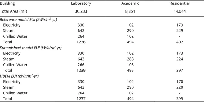
To further investigate the differences between the two models, these retrofit scenario results were evaluated for the representative buildings from Figure 4-7. The three buildings were selected because their measured energy use intensity is closest to the campus average for their respective building type, ensuring that the baseline results from both models closely match. Table 4-8 lists the built-up area for each studied building and compares their baseline annual energy use intensities by utility type against the results from the previously discussed reference model.

Table 4-8: Area details and baseline annual energy use intensities for studied buildings.

Building Laboratory Academic Residential

Total Area (m2₎ _30,233 _8,851 _14,044

Reference model EUI (kWh/m2_-yr)

Electricity 330 102 173

Steam 642 290 229

Chilled Water 264 102 -

Total 1236 494 402

Spreadsheet model EUI (kWh/m2_-yr)

Steam 643 288 224

Total 1239 495 397

UBEM EUI (kWh/m2_-yr)