Effect of distance-dependent dispersivity on density-driven flow in porous media

(1)

HAL Id: hal-03044976

https://hal.archives-ouvertes.fr/hal-03044976

Submitted on 9 Dec 2020

HAL is a multi-disciplinary open access archive for the deposit and dissemination of sci-entific research documents, whether they are pub-lished or not. The documents may come from teaching and research institutions in France or abroad, or from public or private research centers.

L’archive ouverte pluridisciplinaire HAL, est destinée au dépôt et à la diffusion de documents scientifiques de niveau recherche, publiés ou non, émanant des établissements d’enseignement et de recherche français ou étrangers, des laboratoires publics ou privés.

Effect of distance-dependent dispersivity on

density-driven flow in porous media

Anis Younes, Marwan Fahs, Behzad Ataie-Ashtiani, Craig Simmons

To cite this version:

Anis Younes, Marwan Fahs, Behzad Ataie-Ashtiani, Craig Simmons. Effect of distance-dependent dis-persivity on density-driven flow in porous media. Journal of Hydrology, Elsevier, 2020, 589, pp.125204. �10.1016/j.jhydrol.2020.125204�. �hal-03044976�

(2)

1 1

Effect of distance-dependent dispersivity on density-driven flow in

2

porous media

3 4

Anis Younes1,2,3_{, Marwan Fahs}1_{, Behzad Ataie-Ashtiani}4,5_{, Craig T. Simmons}5

5 6

1_{LHyGES, Univ. de Strasbourg/EOST/ENGEES, CNRS, 1 rue Blessig, 67084 Strasbourg, France.}

7

2 _{LISAH, Univ Montpellier, INRA, IRD, Montpellier SupAgro, Montpellier, France.}

8

3 _{LMHE, Ecole Nationale d’Ingénieurs de Tunis, Tunisie}

9

4 _{Department of Civil Engineering, Sharif University of Technology, PO Box 11155-9313, Tehran, Iran}

10

5 _{National Centre for Groundwater Research and Training, College of Science and Engineering, Flinders}

11

University, GPO Box 2100, Adelaide, SA 5001, Australia

12 13 14 15 16 17

Submitted to Journal of Hydrology 18

*Contact person: Marwan Fahs 19

E-mail : fahs@unistra.fr 20

21 22

(3)

2

Abstract

23

In this study, the effect of distance-dependent dispersion coefficients on density-driven flow is 24

investigated. The linear asymptotic model, which assumes that dispersivities increase linearly 25

with distance from the source of contamination and reach asymptotic values at a large 26

asymptotic distance, is employed. An in-house numerical model is adapted to handle distance-27

dependent dispersion. The effect of asymptotic-dispersion on aquifer contamination is analyzed 28

for two tests: (i) a seawater intrusion problem in a coastal aquifer and (ii) a leachate transport 29

problem from a surface deposit site. Global Sensitivity Analysis (GSA) combined with the 30

Polynomial Chaos Expansion (PCE) surrogate modelling is conducted to assess the influence 31

of the dispersion coefficients on the contamination plume for both configurations. 32

For the seawater intrusion problem, the results show that the length of the toe is mainly 33

controlled by the asymptotic transverse dispersivity whereas the spread of the concentration is 34

sensitive to the asymptotic longitudinal dispersivity and the asymptotic dispersivity distance. 35

The latter is the most important parameter controlling the amount of salt which intrudes into 36

the aquifer. For the leachate transport problem, the results show that the asymptotic longitudinal 37

dispersivity coefficient does not affect the concentration distribution. The asymptotic 38

dispersivity distance has a strong effect on the total amount of contaminant that enters the 39

aquifer. This effect can be three times more important than the effect of the asymptotic 40

transverse dispersivity. These findings are likely to be helpful for the investigation and 41

management of density-driven flow problems. 42

Keywords 43

Density driven flow, saltwater intrusion, leachate transport, variable dispersion, asymptotic 44

model, global sensitivity analysis. 45

46 47

(4)

3 1. Introduction

48

Density-driven flow (DDF) is a particular configuration of transport in porous media in which 49

the fluid concentration causes a change in groundwater density which can significantly affect 50

the flow dynamics. DDF can be encountered in several applications related to contaminant 51

transport in aquifers. Among these applications, a well-known problem is the contamination of 52

coastal aquifers by saltwater intrusion (Werner et al., 2013) which is a major concern around 53

the world. Another important example is groundwater contamination by leachates from surface 54

industrial waste and landfills (Frind, 1982). Managing and predicting the evolution of pollutants 55

in such situations require accurate numerical simulations. 56

The simulation of DDF problems is based on coupling Darcy’s groundwater flow equation to 57

the solute transport equation via a state relation expressing the density as a function of solute 58

concentration. Transport of solute in the aquifer is ruled by advection, representing the solute 59

displacement by the mean fluid flow, and by dispersion, which accounts for solute spreading 60

caused by velocity variations due to the heterogeneity of the porous medium at different scales 61

(Liu et Kitandis, 2013; Kitanidis, 2017; Dai et al., 2020). Dispersion processes have been found 62

to play a major role in DDF problems as they cause mixing between different fluids. The effect 63

of dispersion on DDF has been widely investigated in the literature. For instance, Abarca et al. 64

(2007) studied the effect of dispersion on DDF in the context of seawater intrusion and showed 65

that when dispersion is taken into account, concentration isolines resemble those observed in 66

real coastal aquifers. Emami-Meybodi (2017) studied instabilities driven by dispersion for an 67

unstable DDF problem with mixed convective flow. Wen et al. (2018) defined a dispersive 68

Rayleigh number and investigated the effect of dispersion on the Rayleigh-Darcy convection 69

problem. Fahs et al. (2020) investigated the effect of dispersion on thermal DDF problem. 70

In most DDF models, dispersion is ruled using a velocity-dependent dispersion tensor involving 71

constant coefficients characterizing mixing in the longitudinal (parallel to the flow) and 72

(5)

4

transverse (orthogonal to flow) directions. In the last decades, many studies have shown that 73

this conventional approach cannot satisfactorily represent field transport especially for aquifers 74

with spatial heterogeneity (Pickens and Grisak, 1981a). Alternative approaches have developed 75

such as stochastic models (e.g. Gelhar, 1992; Zhang, 2002, Kerrou and Renard, 2010; Pool et 76

al., 2015) or continuous time random walk methods (e.g. Berkowitz et al., 2000; Dentz et al., 77

2004). However, these methods usually require sufficient field measurements to formulate 78

statistical structure and are known to be computationally expensive (Wang et al., 2006). Such 79

difficulties have motivated using the conventional dispersion approach, but by considering that 80

the dispersivity values are temporal or scale dependent (Pickens and Grisak, 1981a). In other 81

words, the longitudinal and transverse dispersion coefficients are not constant but can vary with 82

the distance from the source of contamination. Indeed, in a tracer test, Molz et al. (1983) found 83

that dispersivity is not constant but increases with the travel distance because of the scale 84

dependence of dispersivities. This phenomenon has been observed both in field-scale transport 85

(e.g. Pickens and Grisak 1981a; Gelhar et al., 1992; Schulze-Makuch, 2005) and laboratory-86

scale transport (e.g., Silliman and Simpson, 1987; Khan and Jury, 1990; Huang et al., 1995; 87

Vanderborght and Vereecken, 2007). According to Gao et al. (2012), the scale dependence of 88

dispersivity can be related to different processes such as the heterogeneity of the porous media 89

at different scales (Gelhar et al., 1992; Huang et al., 2006), the fractal nature of the pore space 90

in the aquifer (Wheatcraft and Tyler, 1988) or the anomalous transport (Cortis and Berkowitz, 91

2004). Mishra and Parker (1990) showed that a hyperbolic dispersivity-distance function allows 92

a good fitting of the data estimated from a natural gradient tracer experiment. Kangle et al. 93

(1996) provided a one-dimensional analytical solution with linear asymptotic dispersion. Chen 94

et al. (2003, 2007) investigated distance-dependent dispersion for convergent and divergent 95

flow fields with linear scale-dependent dispersion. Chen et al (2008a) studied one-dimensional 96

transport with hyperbolic asymptotic dispersivity function. Pérez Guerrero and Skaggs (2010) 97

(6)

5

derived a general analytical solution for one-dimensional transport with distance-dependent 98

coefficients. Gao et al. (2010, 2012) investigated mobile-immobile transport model with 99

asymptotic scale-dependent dispersivity. You and Zhan (2013) developed semi-analytical 100

solutions for solute transport in a finite column with linear asymptotic and exponential distance-101

dependent dispersivities and time-dependent sources. 102

Thus, in the literature, the effect of asymptotic dispersivity has been essentially investigated for 103

simplified situations of 1D transport (e.g. Basha and El-Habel, 1993; Yates, 1992; David-104

Logan, 1996; Pang and Hunt, 2001; Chen et al., 2003; Pérez Guerrero and Skaggs, 2010; 105

Sharma and Abgaze, 2015, Wang et al., 2019), 2D problems with a uniform flow field (e.g. 106

Hunt, 2002; Chen et al., 2008b) or radially convergent divergent flow fields (e.g. Chen et al., 107

2003, 2006, 2007). To the best our knowledge, investigation of distance-dependent dispersion 108

coefficients in cases involving complex velocity fields, such as in DDF problems, have not been 109

undertaken. 110

The aim of this work is to incorporate distance-dependent dispersion in a DDF model and to 111

investigate the effect of dispersion parameters on contaminant transport. As conceptual models, 112

we consider (i) the Henry problem describing seawater intrusion (SWI) in a coastal aquifer 113

(Henry, 1964) and (ii) the leachate transport problem proposed by Frind (1982) to investigate 114

the leachate plume from a surface deposit site. The effect of distance-dependent dispersivities 115

on the aquifer contamination is investigated using Global Sensitivity Analysis (GSA) combined 116

with Polynomial Chaos Expansion (PCE) surrogate modelling (Sudret, 2008; Fajraoui et al., 117

2012, 2017; Mara et al., 2017). 118

2. Methods 119

2.1 The mathematical model and numerical code

120

The mathematical model for water movement through porous media is based on the mass 121

conservation equation and Darcy’s law (Guevara et al., 2015): 122

(7)

6 0 h C S t C t



 











 

  q (1) 123 0 0 0g _h _z           _   _   q k (2) 124

where  is the fluid density [ML-3], S the specific mass storativity related to head changes [L -125

1_],

h the equivalent freshwater head [L], t the time [T],  the porosity [-], C the relative 126

concentration [-], q the Darcy’s velocity [LT-1], ₀ the density of the displaced fluid [ML-3], 127

g

the gravity acceleration [LT-2],



the fluid dynamic viscosity [ML-1T-1], k the permeability

128

tensor [L2] and z the depth [L] taken positive upwards. 129

The contaminant transport in porous media is based on the solute mass conservation equation: 130 0 ( C ) .( C . C ) t

 

_



  q D  (3) 131

where the dispersive tensor

D

is given by: 132





T m L T T D / D I

 

 qq q



q I (4) 133

with _L and _T the longitudinal and transverse dispersion coefficients [L], D the pore water _m

134

diffusion coefficient [L2_T-1_{] and}

_I

_{the unit tensor. The associated boundary conditions of the}

135

flow-transport system (1)-(3) are of Dirichlet, Neuman or mixed type. 136

Flow and transport equations are coupled via the linear mixture density equation: 137





0 1 0 C

 

 

 

 (5)

138

where ₁ is density of contaminant. 139

In this work, we assume that the longitudinal and transverse dispersion coefficients are a 140

function of the distance from the source of contamination. Distance-dependent dispersivities 141

are generally ruled using one of the four types of functions suggested by Pickens and Grisak 142

(1981b) including linear, parabolic, asymptotic and exponential functions. The linear distance-143

dependent dispersivity function has been largely used in the literature (e.g. Pang and Hunt, 144

(8)

7

2001; Gao et al., 2010; Pérez Guerrero and Skaggs, 2010; Chen et al., 2008b). However, this 145

function seems to be unphysical, because field observations show that a constant dispersivity 146

could be asymptotically reached (Gelhar et al., 1992; Pickens and Grisak, 1981a). Huang et al. 147

(1995) used a linear-asymptotic distance-dependent function where the dispersivity value 148

increases linearly with the transport distance and reaches an asymptotic value at a certain large 149

distance. The linear-asymptotic model was adopted by You and Zhan (2013) and is employed 150 in this work: 151

 

0 0 0 0 0 0 L ,T L ,T L ,T , ,     _{ }     _  x (6) 152

where corresponds to the distance from the source of contamination, 0

L

 and 0

T

 are 153

respectively the asymptotic longitudinal and transverse dispersion coefficients and ₀ is the 154

asymptotic distance after which both longitudinal and transverse dispersivities reach their 155

asymptotic values 0

L ,T L ,T

  .

156

The coupled flow-transport system is solved with an advanced in-house numerical model using 157

triangular meshes (Ackerer and Younes, 2008). The flow equations (Eqs. 1-2) are solved by the 158

mixed finite element method (Younes et al., 2010). The transport equation (Eq. 3) is solved by 159

combining two numerical methods: Discontinuous Galerkin (DG) method for solving advection 160

and Multipoint Flux Approximation (MPFA) method for solving dispersion. Coupling between 161

flow and transport equations is performed using the non-iterative scheme proposed in Younes 162

and Ackerer (2010) with proper time management. This scheme was shown to be highly 163

efficient and more accurate than the standard iterative procedure. The in-house code has been 164

validated by comparison against semi-analytical solutions in Fahs et al. (2016). Performance 165

and robustness of the code has been highlighted in Shao et al. (2018) by comparison against 166

COMSOL Multiphysics. In this work, the in-house code is modified to handle distance-167

(9)

8

dependent dispersion coefficients. Both longitudinal and transverse dispersivities are defined 168

elementwise and their values are calculated using (Eq. 4) where corresponds to the distance 169

from the center of each element to the source of contamination. 170

171

2.2 The Henry saltwater Intrusion Problem

172

Real applications of SWI at a field scale are increasingly reported in the literature. However, in 173

several theoretical and applied studies, SWI is often investigated based on the hypothetical 174

Henry problem (Henry, 1964) (Figure 1a). This problem represents a common benchmark that 175

is widely used for multiple purposes as understanding physical processes, numerical model 176

verification, and parameter sensitivity analyses. A detailed review of the different use of the 177

Henry problem as a surrogate representation of SWI can be found in Werner et al. (2013) and 178

Fahs et al. (2018). 179

The Henry problem represents SWI in a vertical cross-section of a confined coastal aquifer 180

where an inland freshwater flow is in equilibrium with seawater that intrudes into the aquifer 181

from the seaside due to its higher density (Figure 1a). The first studies on the Henry problem 182

have been limited to pure molecular diffusion cases. More realistic configurations that include 183

velocity-dependent dispersion have been suggested in Abarca et al. (2007) and Fahs et al. 184

(2016). These cases will be considered here as this work deals with asymptotic dispersion 185 coefficients. 186 187 188 189 190 191 192

(10)

9 193

(a)

(b)

Figure 1. (a) Henry problem domain and boundary conditions; (b) The leachate transport 194

problem (Frind, 1982). 195

196

Following Simpson and Clement (2004), we decrease the freshwater recharge by half to 197

increase the density-dependent effects compared to boundary forces. Further, we use a larger 198

rectangular domain with an aspect ratio L 3

H  as proposed by Zidane et al. (2012) to reduce

199

the influence of the left boundary condition on the saltwater distribution. The parameters and 200

boundary conditions for the Henry problem are given in Table 1. 201 202 203 204 205 3m 1m x z 3000m x 120m 920m 24m z

(11)

10 206

207 208 209

Table 1. Parameters and boundary conditions for the Henry problem. 210

permeability k= 1.0204 x 10-9 m2

porosity

length of the aquifer height of the aquifer

0.35   3 L m 1 H m

-molecular diffusion coefficient 8

9.4 10 m

D    m2 s-1

Boundary conditions for flow - hydrostatic pressure at the right hand side

- constant flux at the inland boundary: Q3.3 10 5 m2/s - no flow along the top and bottom

Boundary conditions for transport _- 0

 = 1000 kg/m3 on the left boundary. - ₁ = 1025 kg/m3 on the right boundary

- zero concentration gradient along the top and bottom 211

The numerical model is employed to analyze the saltwater intrusion by considering that 212

uncertainty of model outputs is associated with the following dispersion parameters: the 213

asymptotic longitudinal dispersivity L0, the asymptotic transverse dispersivity

0

T

 and the 214

asymptotic distance ₀. Note that the longitudinal and transverse dispersivities are assumed to 215

be independent. The corresponding uncertainty ranges (Table 2) are sufficiently large to explore 216

the role of each parameter. 217

Table 2. Uncertainty ranges of the dispersion coefficients for the Henry problem. 218

Parameter Uncertainty Range

0 L  [m] [0.1, 1.0] 0 T  [m] [0.04, 1.0] 0 [m] [0, 2.0] 219

(12)

11

2.3 The leachate transport problem in unconfined aquifer

220

This problem was proposed by Frind (1982) to investigate groundwater contamination by 221

leachates from sanitary landfills or industrial waste disposal sites. A typical problem is 222

considered (Figure 1b) where a disposal site unprotected from precipitation is situated above 223

the water table in a rectangular unconfined aquifer of 3000 m length and 24m thickness. 224

The parameters and boundary conditions are described in Table 3. 225

Table 3. Parameters and boundary conditions for the leachate transport problem. 226

- permeability kx= 0.3262 x 10-10 m2

kz= 0.3262 x 10-11 m2

- porosity

- length of the aquifer - height of the aquifer

0.2   3000 L m 24 H m

- molecular diffusion coefficient _0.0

m

D  m2 s-1

- boundary conditions for flow - fixed head at the left (h0=0) and right (hL=-17.5m) hand

sides

- constant flux at the top: q_z 30cm/year - no flow along the bottom

- boundary conditions for transport - fixed relative concentration (C=C0) at the top with C0=1 for x1 x x2

C0=0 elsewhere

with x₁120m and x₂ 920m

- fixed relative concentration (C=0) at the left and right hand sides

- density of the contaminant ₁1007.1 kg/m3

- zero concentration gradient along the bottom 227

Large uncertainty ranges (Table 4) are associated to the dispersion parameters (L0,

0

T

 and ₀

228

) in order to investigate the role of each of them. Note that because the leachate transport 229

problem has larger dimensions than the synthetic Henry problem, the dispersion parameters are 230

allowed to have larger values than previously. 231

232 233

(13)

12 234

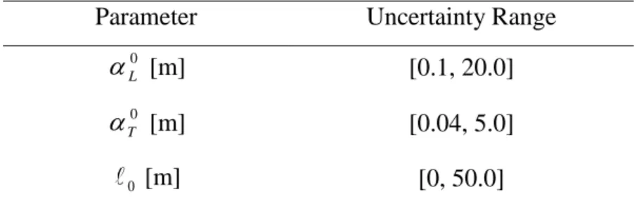
Table 4. Uncertainty ranges of the dispersion parameters for the leachate transport problem. 235

Parameter Uncertainty Range

0 L  [m] [0.1, 20.0] 0 T  [m] [0.04, 5.0] 0 [m] [0, 50.0] 236

3. Global sensitivity analysis

237

Effect of the dispersion parameters on DDF is investigated using global sensitivity analysis 238

(GSA). To this aim, the variance-based sensitivity indices of Sobol’ (Sobol’, 2001) are 239

computed using Polynomial Chaos Expansion (PCE). The Sobol’ indices measure the 240

contribution of an input (alone or by interactions with other inputs) to the output variance. They 241

are well adapted for GSA since they do not require any assumption of monotony or linearity of 242

the model (Saltelli et al., 2006). Two Sobol’ indices are noteworthy: 243

- the first-order sensitivity index, 244

 

i _i i V E y _V S V y V    _ _     (4) 245

- the total sensitivity index, 246

 

T i _i i E V y _V ST V y V   _ _      (5) 247

where y is the model output,  is the set of parameters  



 _L0, _T0, ₀



, E

 

is the 248

mathematical expectation (the average), V

 

is the mathematical variance, E _{ } and V _{ }

249

are their respective conditional forms. _i represents one of the parameters, and __i stands for 250

the set of parameters  without the parameter _i. 251

(14)

13

The first-order sensitivity index (or main effect index) S_i

 

0,1 measures the amount by which 252

the variance of y is reduced when the true value of _i is known. The total sensitivity index 253

 

0,1

i

ST  measures the remaining uncertainty in y after all parameters are known except _i. 254

It evaluates the contribution of _i to the response variance, including its interactions with the 255

other parameters (i.e., _~i). If interactions between parameters are negligible, we have i 1

i S 



256 and S_i ST_i ,i. 257

The marginal effect y

 

_i of the parameter _i on the model output y enables to investigate 258

the range of variation of y with respect to _i, 259

 

i i

y     E y_ _. (7)

260

In this work, we use the Polynomial Chaos Expansion (PCE) surrogate modeling to infer 261

sensitivity indices (Fajraoui et al., 2012, 2017; Younes et al., 2016; Shao et al., 2017). PCE 262

allows an efficient evaluation of the Sobol’ indices, since they can be easily calculated using 263

the PCE coefficients (Sudret, 2008). 264

Since we deal with only three uncertain parameters (L0,

0

T

 and ₀), we use a full surrogate 265

PCE of order 4. The number of polynomial coefficients in the expansion is therefore 7! 35 4! 3! 

266

. The coefficients of the surrogate PCE are calculated by a least-square technique minimizing 267

the sum of squared errors between model responses and the PCE. To this aim, a hundred of 268

evaluations of the Henry and leachate transport problems are performed using parameter values 269

randomly generated in the intervals of variation given in Table 2 and Table 4 respectively. 270

4. Results for the Henry SWI problem 271

(15)

14

A mesh converged solution is obtained a uniform triangular mesh formed by 4800 elements. 272

The effect of the dispersion parameters on saltwater intrusion is investigated based on the 273

following metrics (see Figure 2). 274

- The positions X_0.1,X_0.5 and X_0.9 of respectively the 10%, 50% and 90% isochlors at 275

the aquifer bottom. Note that the X_0.5 is related to the well-known length of the toe L _toe

276

which is the distance between the seaside boundary and X_0.5. 277

- The spread of the concentration L_S  X_0.9X_0.1 which corresponds to the distance 278

between the 10% and the 90% isochlors at the bottom of the domain. 279

- The total mass in the domain. 280

- The values of steady state concentration at the following selected points: A₁



1.5, 0



; 281





2 2.5, 0 A and A₃



2.5,1



. 282 283 284

Figure 2. Seawater intrusion metrics used for the assessment of effects of the dispersion 285 parameters. 286 287 4.1 Salinity distribution 288

Figure 3a depicts the mean concentration values as well as the corresponding 10%, 50% and 289

90% concentration contours. This figure shows that the distribution of the mean concentration 290

reflects the general distribution of salinity in coastal aquifers which gives confidence to the 291

accuracy of the PCE surrogate model. Saltwater intrudes from the right and reaches equilibrium 292

(16)

15

with the inland freshwater flow. Saltwater intrusion is more pronounced near the bottom 293

because of density effects. The mean concentration distribution in Figure 3a shows a wide 294

mixing zone due to the large uncertainty ranges of the dispersion parameters (Table 2). 295

296

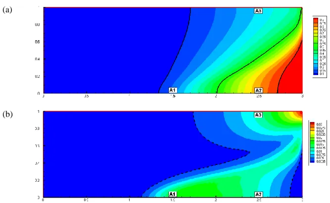
(a)

(b)

Figure 3. The Henry problem: (a) Spatial map of the mean concentration values (black lines 297

represent 90%, 50% and 10% isochlors); (b) Spatial map of the variance of concentrations 298

(dashed lines limit the zone of high variability- 5% of standard deviation). 299

300

The distribution of the variance of the concentration shows that high variances regions are 301

located at the center of the domain near the bottom of the aquifer (Figure 3b). This makes sense 302

as the length of the toe is mainly controlled by the dispersion processes (Abarca et al., 2007; 303

Fahs et al., 2016). Indeed, it is well known that low dispersion increases the buoyancy forces 304

compared to dispersion effects and yields much more intrusion near the bottom of the aquifer 305

(Younes and Fahs, 2014). This explains the high variance region near A1 in Figure 3b. 306

Significant variability of the salinity can be observed also at top of the aquifer near the seaside 307

(Figure 3b). In this zone, the groundwater flow is discharging to the sea. Thus, the salinity of 308

(17)

16

this zone is mainly due to dispersion. The dashed contour in Figure 3b shows the region where 309

the effect of dispersion parameters is significant which corresponds to 5% of the standard 310

deviation of the concentrations. 311

312

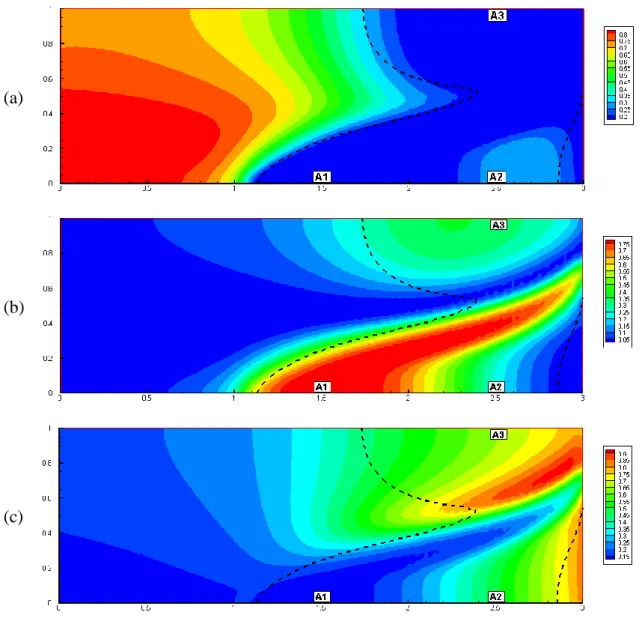
The spatial maps of first order Sobol’ indices representing the sensitivity of the salinity 313

distribution to 0

L

 , 0

T

 and ₀ are plotted in the Figure 4. For the region of significant variance 314

(the region delimited by the dashed lines), Figure 4a shows that _L0 has a negligible effect on 315

salinity distribution, except around A2 where a moderate effect can be observed. The parameter 316

0

T

 is the most influential parameter as its zone of high sensitivity is situated in the region of 317

high variability (Figure 4b). Significant sensitivity to 0

T

 is observed around A3 but the highest 318

sensitivity area is situated in the mixing zone near A1. This is in agreement with the results of 319

Fahs et al. (2016) and is related to the fact that in this zone, the velocity field is not parallel to 320

the concentration gradient. As shown in Fahs et al. (2016), in such a case, the dispersion 321

processes are dominated by the transverse dispersion and hence, the salinity distribution is 322

highly sensitive to T0 in this zone. The parameter 0 is influential near the seaside boundary 323

(Figure 4c) which makes sense since, far from the sea, the longitudinal and transverse dispersion 324

coefficients reach their asymptotic values and the salinity distribution become insensitive to ₀ 325 . 326 327 328 329 330 331 332

(18)

17 (a) (b) (c) Figure 4. Spatial maps of the first-order sensitivity indices: (a) sensitivity of salinity 333

distribution to 0

L

 , (b) sensitivity of salinity distribution to 0

T

 and (c) sensitivity of salinity 334

distribution to ₀. Dashed lines limit the zone of high variability (5% of standard deviation). 335

336

4.2 Sensitivity of the SWI metrics

337

The Sobol’ indices for the concentration at the observation points (A1, A2, A3) as well as for 338

the SWI metrics are depicted in Table 5. This table also gives the mean value and the standard 339

deviation for all quantities of interest. 340

Table 5. Sensitivity of the concentration at the observation points (A1, A2 and A3) and of 341

the SWI metrics. S , ₁ S and ₂ S represent the first order Sobol’ indices for the sensitivity to ₃

(19)

18 0

L

 , 0

T

 and ₀. ‘mean’ and ‘std’ represent the mean value and the standard deviation for the 343 quantities of interest. 344 345 mean std S 1 S 2 S 3 3 1 i i S 



A1 0.17 0.12 0.01 0.81 0.04 0.86 A2 0.79 0.1 0.27 0.24 0.42 0.94 A3 0.27 0.11 0.02 0.33 0.6 0.95 0.1 X 1.39 0.17 0.13 0.64 0.06 0.82 0.5 X 2.0 0.19 0.07 0.73 0.13 0.93 0.9 X 2.66 0.19 0.30 0.16 0.46 0.93 S L 1.27 0.23 0.5 0.05 0.41 0.97 Total mass 1016 110 0.16 0.16 0.35 0.67 346

The results of this table show that 347

- The concentration near A1 is mostly influenced by T0



S2 0.81



. In this region, 348

moderate interactions occur between parameters 3 1 0.86 i i S       



. The effects of 0 L  and 349

0 alone are insignificant



S2 0.01 and S3 0.04



, but their total effects (including 350

interactions) are moderately significant



ST₁ 0.12 and ST₃0.11



. The results around 351

A1 are coherent with the results discussed previously based on the spatial maps of 352

Sobol’ indices (Figure 4). 353

- Around A2, located near the sea boundary, high concentrations can be observed 354

(mean=0.79). The concentration has slight variability (std=0.1) which indicates that 355

SWI reaches this point whatever the values of the dispersion parameters. The most 356

influential parameter near A2 is ₀



S₃0.42



. The parameters _L0 and _T0 have 357

(20)

19

significant and close effects



S₁ 0.27and S₂ 0.24



. Interactions between dispersion 358

parameters are not significant 3 1 0.94 i i S   _    



. 359

- The point A3 is located near the top of the domain and close to the sea boundary. The 360

standard deviation (std=0.11) of concentrations is relatively significant (mean=0.27). 361

The most influential parameter in this region is ₀



S₃0.6



20 parameters 3 1 0.93 i i S   _   





. Therefore, X0.5 and in consequence Ltoe are mainly

378

controlled by the asymptotic transverse dispersivity. Since interactions are small, the 379

marginal effect of 0

T

 , depicted in the Figure 5a, reflects the behavior of X_0.5 when 380

varying 0

T

 (the other parameters are set at their mean values). Figure 5a shows a high 381

sensitivity for _T0 0.3 and a weaker sensitivity for higher values of _T0. In this figure, 382

0.5

X increases with T0 which is consistent with physics as the decrease in

0

T

 induces

383

more saltwater intrusion and hence a decrease of X_0.5. 384

Figure 5. Marginal effect of: (a) T0 on X0.5, (b)

0 L  on X_0.9, (c) T0 on X0.9, (d) 0 on 385 0.9 X , (e) _L0on L and (f) _S ₀ on L _S 386 387

- The 90% isochlor intersects the substratum at an average distance of 2.66 m with a 388

standard deviation of 0.19 m. X_0.9 is sensitive to the three dispersion parameters. As the 389

isochlor 90% is close to the sea, the most influential parameter is ₀



S₃0.46



, comes 390 next 0 L 



S10.30



and finally 0 T





S2 0.16



. Small interactions exist between the 391

(22)

21 dispersion parameters 3 1 0.93 i i S   _   





. Marginal effects of the three sensitive dispersion

392

parameters on X_0.9 are plotted in the Figure 5. The sensitivity of X_0.9 to 0

L

 (Figure 5b) 393

has a positive slope as an increase of _L0 induces an increase of the spreading of the 394

concentration front resulting in an increase of X_0.9. The sensitivity of X_0.9 to _T0 (Figure 395

5c) is similar to that observed for X_0.5. This demonstrates that saltwater intrusion is 396

mainly controlled by the asymptotic transverse dispersivity. A decrease of 0

T

 induces

397

more intrusion which results in a decrease of X_0.5 and X_0.9. The sensitivity of the 398

intrusion to T0 is more pronounced for small values of this parameter. The X0.9 varies

399

almost linearly with a negative slope with respect to the parameter ₀ (Figure 5d). 400

Indeed, the 90% isochlor is located near the sea boundary (the average X_0.9 is 2.66m) 401

where the effect of ₀ is significant (see Figure 4c). In that region, the increase of ₀ 402

yields less dispersion effects which results in more saltwater intrusion and hence a 403

decrease in X_0.9. 404

- For the spread of the concentration (Ls), the most influential parameter is L0



S10.5



405

, followed by ₀



S₃0.41



. The sensitivity of L to _S 0

L

 is much more important than

406

that of X_0.1 and X_0.9. Furthermore, although T0 is influential on X0.9 and on X0.1, it 407

has no effect on L _S



S₂ 0.05



. The interactions between parameters are almost absent 408 3 1 0.97 i i S   _   





. The marginal effects of the parameters

0

L

 and ₀ on L are depicted _S

409

in the Figure 5. L increases linearly with the value of _S L0 (Figure 5e). This confirms

410

that the spreading is directly proportional to the value of L0. The sensitivity of L to S

(23)

22

0 has a negative slope (Figure 5f). The increase of 0 yields less dispersion which 412

results in less spreading of the concentration front and hence a reduction in L . _S

413

- The standard deviation of the total mass in the aquifer is around 10% of its mean value. 414

Significant interactions occur between the dispersion parameters 3 1 0.67 i i S   _    



. The 415

total sensitivity indices of the three dispersion parameters



ST₁0.46, ST₂ 0.23 and 416



3 0.64

ST  are significantly higher than their first order indices



S₁0.16, S₂ 0.16 417

and S₃0.35



. This shows that ₀ plays the most important role on the amount of mass 418

which has intruded into the domain, followed by _L0. Strong interactions mainly occur 419

between these two parameters since ST₃S₃0.29 and ST₁ S₁ 0.3 whereas 420

2 2 0.07

ST S  . 421

5. Results of the leachate transport problem 422

Starting with no leachate in the aquifer, the leachate transport problem is simulated for 24 years. 423

A mesh converged solution is obtained using a uniform triangular mesh formed by 14400 424

triangular elements. A hundred simulations were performed using independent random 425

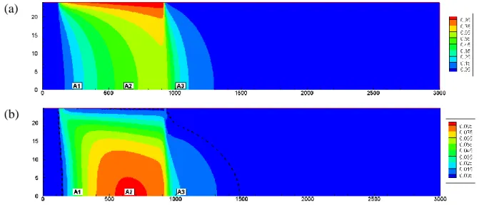
parameter values generated inside the intervals given in Table 4. The mean leachate plume is 426

shown in the Figure 6a. The leachate enters the aquifer due to dispersion and vertical infiltration. 427

Within the aquifer, the leachate plume moves to the right side due to the hydraulic gradient 428

between left and right sides. A stable flow is obtained for all explored dispersivity values 429

because of (i) the large dispersion and (ii) the weak density difference between the contaminant 430 and freshwater. 431 432 433 434

(24)

23 (a)

(b)

435

Figure 6. The leachate transport problem at 24 years: (a) Spatial map of the mean concentration 436

values and (b) Spatial map of variance of concentration. The dashed contour delimits the region 437

of high variances (5% of standard deviation). 438

439

The distribution of the variance of the concentration shows that high variability is located below 440

the disposal site (Figure 6b) towards the bottom of the aquifer. The center of the zone of high 441

variability is shifted to the right of the disposal site center because of the basic advective flow 442

in the aquifer which goes from left to right. 443

Figure 7 shows the spatial distributions of the first-order Sobol’ indices. For the region of 444

significant variability (delimited by dashed lines), the asymptotic longitudinal dispersivity L0

445

has a negligible first-order sensitivity index (Figure 7a). Note that this does not imply the 446

irrelevance of _L0 since the first-order index does not take into account interactions between 447

parameters. To judge the inefficiency of _L0, we evaluate the total Sobol index of _L0. Figure 448

8 shows that, in the region of high variance,L0 has no effect on the concentration distribution

449

(neither alone nor in interaction with the other parameters). Therefore, the parameter L0 is

450

irrelevant for concentration distribution. Thus, in this case, mixing by dispersion is mainly 451

related to transverse dispersivity. The parameters T0 and 0 have strong influence on the 452

concentration distribution (Figure 7b and 7c) in the region of high variability (below the landfill 453

(25)

24

site). Significant interactions are observed between these two parameters. The amount of 454

interaction between parameters can be evaluated by computing 1 i

i

r 



S . If interactions 455

between parameters are absent, then _i 1

i

S 



and r0. Figure 9 shows that interactions 456

between T0 and 0 are observed in two regions located in the lower half of domain. Moderate 457

interactions occur in the region between x = 100 m and x = 500 m. Higher interactions occur in 458

a larger zone located downstream the deposit site between x = 1000 m and x = 1500m. 459

460

461

462

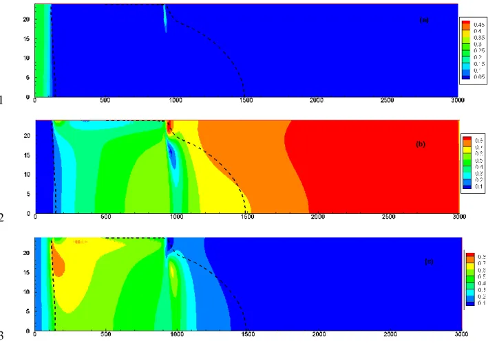
463

Figure 7. Spatial map of the first order sensitivity indices for the leachate transport problem: 464 a) sensitivity to L0, b) sentitivity to 0 T  and c) sensitivity to ₀. 465

(26)

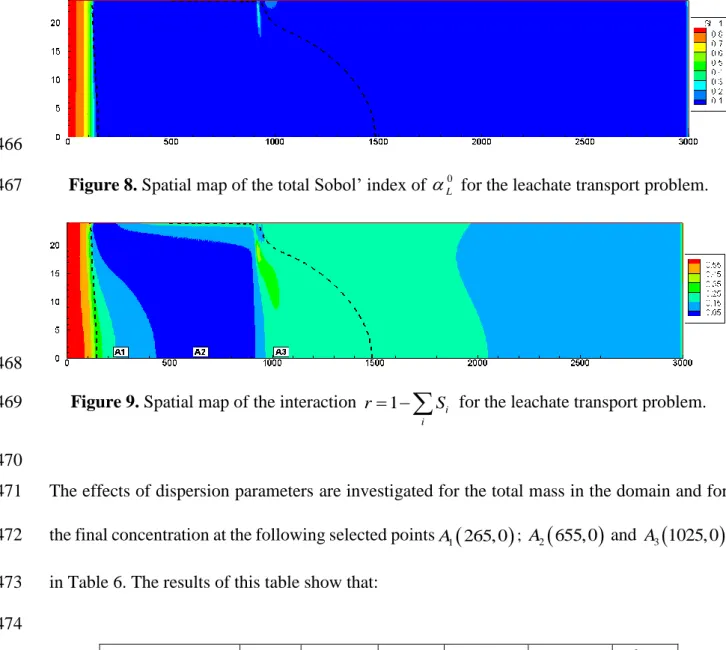
25 466

Figure 8. Spatial map of the total Sobol’ index of L0 for the leachate transport problem.

467

468

Figure 9. Spatial map of the interaction 1 _i

i

r 



S for the leachate transport problem. 469

470

The effects of dispersion parameters are investigated for the total mass in the domain and for 471

472

in Table 6. The results of this table show that: 473 474 mean std S 1 S 2 S 3 3 1 i i S 



A1 0.19 0.2 0.0 0.29 0.58 0.87 A2 0.52 0.3 0. 0.51 0.46 0.97 A3 0.29 0.13 0.0 0.37 0.39 0.76 Total mass 10667 4058 0.0 0.24 0.74 0.98 475

Table 6. Sobol’s indices for the concentration at the observation points (A1,..,3) and for the

476

total mass in the domain for the leachate transport problem. S , ₁ S and ₂ S represent the first ₃

477

order Sobol’ indices for the sensitivity to 0

L

 , _T0 and ₀. ‘mean’ and ‘std’ represent the 478

mean value and the standard variation for the quantities of interest. 479

(27)

26



S2 0.51



and 0 483



S3 0.46



. In this region, the model is almost additive since interactions between 484

parameters are almost absent 3 1 0.97 i i S   _    



. 485

- Around A3, the parameters T0 and 0 have close first-order sensitivity indices 486



S2 0.37 and S30.39



and close total sensitivity indices



ST2 0.6 and 487



3 0.63

ST  . In this region, strong interactions occur between these two parameters 488 3 1 0.76 i i S   _    



. 489

. The effects of the two parameters are additive since interactions 493

between them are almost absent 3 1 0.98 i i S   _   





. The marginal effects of the parameters

494

0

T

 and ₀ on the total mass are plotted in Figure 10. The sensitivity of the total mass 495

to T0 depicts a curve with a positive slope since the total mass increases as

0

T 

496

increases. The marginal effect of ₀ is represented by a negative slope curve which is 497

consistent with physics. The leachate plume, and consequently the total mass, increase 498

as dispersion increases (i.e. ₀ decreases). 499

(28)

27 500

Figure 10. Marginal effects of _T0, and ₀ on the total mass for the leachate transport 501

problem. 502

6. Conclusions 503

Transport of pollutants in aquifers is usually modeled using the advection-dispersion transport 504

equation with constant-dispersion coefficients. Recently, laboratory and field transport 505

observations have shown that dispersivities are distance-dependent. The most popular function 506

for distance-dependent dispersivity is the linear-asymptotic model which assumes that the 507

longitudinal and transverse dispersion coefficients increase linearly with the distance from the 508

source of contamination until some asymptotic distance ₀, after which the dispersion 509

coefficients reach asymptotic values. In the literature, this model has been investigated in 510

simple configurations dealing with either one-dimensional or uniform two-dimensional flow 511

fields. In this work, we investigate the effects of asymptotic dispersion model in the case of 512

contaminant transport with DDF that involves complex velocity field. The linear-asymptotic 513

model has been incorporated in an advanced in-house DDF numerical model. The new 514

developed code was used to investigate the effect of the dispersion coefficients (asymptotic 515

longitudinal dispersivity _L0, asymptotic transverse dipersivity _T0 and asymptotic distance ₀ 516

) on the contamination plume for two conceptual models: the Henry saltwater intrusion problem 517

and a leachate transport problem from a surface deposit site. The effects of dispersion 518

parameters are evaluated using Global Sensitivity Analysis (GSA) combined with the 519

(29)

28

Polynomial Chaos Expansion (PCE) surrogate modelling to compute both first-order and total 520

Sobol’ sensitivity indices 521

The results for the Henry problem showed that the concentration at the center bottom of the 522

domain, is mostly influenced by the asymptotic value of the transverse dispersion 0

T

 whereas, 523

near the sea boundary, the most influential parameter is the asymptotic distance ₀. The 524

position of the 50% isochlor is mainly controlled by the parameter T0. The spread of the

525

concentration is not influenced by T0 but by

0

L

 and ₀. The total amount of mass intruded in 526

the aquifer is influenced by ₀ and then by L0 and interactions between them.

527

The results for the leachate transport problem show that L0 has no effect (neither alone nor in

528

interaction with the other parameters) on the concentration distribution. The parameters T0

529

and ₀ have a strong influence on the concentration distribution below the landfill site. Strong 530

interactions occur between these two parameters in the aquifer. The total mass in the aquifer is 531

strongly influenced by ₀. The sensitivity to ₀ is three times more important than to T0 and

532

the effects of these two parameters on the total mass are additive (interactions are insignificant). 533

This study showed that distance-dependent dispersion coefficients can significantly affect 534

contaminant distribution in aquifers in the case of density-driven flow. It demonstrates the 535

advantage of using GSA with PCE surrogate modeling for such investigation since it allows to 536

determine, for each parameter, the regions of high influence and the regions where the effect of 537

the parameter is insignificant. It also allows to determine regions of high interactions between 538

parameters and to explore the marginal effect of sensitive parameters on the model output. 539

540 541 542 543

(30)

29 Acknowledgments

544

This work was partially supported by the Tunisian-French joint international laboratory NAILA 545

(http://www.lmi-naila.com/). Marwan Fahs would acknowledge the support from the national 546

school of water and environmental engineering of Strasbourg through the research project 547

PORO6100. Behzad Ataie-Ashtiani and Craig T. Simmons acknowledge support from the 548

National Centre for Groundwater Research and Training, Australia. Behzad Ataie-Ashtiani also 549

appreciates the support of the Research Office of the Sharif University of Technology, Iran. 550

The data used in this work are available on the GitHub repository: https://github.com/fahs-551

LHYGES 552

553

(31)

30 References 554

1. Abarca, E., Carrera, J., Sánchez-Vila, X., & Dentz, M. (2007). Anisotropic dispersive Henry 555

problem. Advances in Water Resources, 30(4), 913–926.

556

https://doi.org/10.1016/j.advwatres.2006.08.005 557

2. Ackerer, P., & Younes, A. (2008). Efficient approximations for the simulation of density 558

driven flow in porous media. Advances in Water Resources, 31(1), 15–27. 559

3. Basha, H. A., & El-Habel, F. S. (1993). Analytical solution of the one-dimensional time-561

dependent transport equation. Water Resources Research, 29(9), 3209–3214. 562

https://doi.org/10.1029/93WR01038 563

4. Berkowitz, B., Scher, H., Silliman, S.E., 2000. Anomalous transport in laboratory-scale, 564

heterogeneous porous media. Water Resour. Res. 36, 149–158.

565

https://doi.org/10.1029/1999WR900295 566

5. Chen, J.-S., Liu, C.-W., Hsu, H.-T., & Liao, C.-M. (2003). A Laplace transform power 567

series solution for solute transport in a convergent flow field with scale-dependent 568

dispersion. Water Resources Research, 39(8). https://doi.org/10.1029/2003WR002299 569

6. Chen, J.-S., Liu, C.-W., & Liang, C.-P. (2006). Evaluation of longitudinal and transverse 570

dispersivities/distance ratios for tracer test in a radially convergent flow field with scale-571

dependent dispersion. Advances in Water Resources, 29(6), 887–898.

572

7. Chen, J.-S., Chen, C.-S., & Chen, C. Y. (2007). Analysis of solute transport in a divergent 574

flow tracer test with scale-dependent dispersion. Hydrological Processes, 21(18), 2526– 575

2536. https://doi.org/10.1002/hyp.6496 576

8. Chen, J.-S., Ni, C.-F., Liang, C.-P., & Chiang, C.-C. (2008a). Analytical power series 577

solution for contaminant transport with hyperbolic asymptotic distance-dependent 578

dispersivity. Journal of Hydrology, 362(1–2), 142–149.

579

https://doi.org/10.1016/j.jhydrol.2008.08.020 580

9. Chen, J.-S., Ni, C.-F., & Liang, C.-P. (2008b). Analytical power series solutions to the two-581

dimensional advection-dispersion equation with distance-dependent dispersivities. 582

Hydrological Processes, 22(24), 4670–4678. https://doi.org/10.1002/hyp.7067

583

10. Cortis, A., & Berkowitz, B. (2004). Anomalous Transport in “Classical” Soil and Sand 584

Columns. Soil Science Society of America Journal, 68(5), 1539–1548.

585

https://doi.org/10.2136/sssaj2004.1539 586

11. Dai, Z., Zhan, C., Dong, S., Yin, S., Zhang, X., & Soltanian, M. R. (2020). How does 587

resolution of sedimentary architecture data affect plume dispersion in multiscale and 588

hierarchical systems? Journal of Hydrology, 582, 124516.

589

https://doi.org/10.1016/j.jhydrol.2019.124516 590

12. David Logan, J. (1996). Solute transport in porous media with scale-dependent dispersion 591

and periodic boundary conditions. Journal of Hydrology, 184(3–4), 261–276. 592

https://doi.org/10.1016/0022-1694(95)02976-1 593

13. Dentz, M., Cortis, A., Scher, H., Berkowitz, B., 2004. Time behavior of solute transport in 594

heterogeneous media: transition from anomalous to normal transport. Advances in Water 595

Resources 27, 155–173. https://doi.org/10.1016/j.advwatres.2003.11.002 596

14. Emami-Meybodi, H. (2017). Dispersion-driven instability of mixed convective flow in 597

porous media. Physics of Fluids, 29(9), 094102. https://doi.org/10.1063/1.4990386 598

15. Fahs, M., Ataie-Ashtiani, B., Younes, A., Simmons, C. T., & Ackerer, P. (2016). The Henry 599

problem: New semianalytical solution for velocity-dependent dispersion. Water Resources 600

Research, 52(9), 7382–7407. https://doi.org/10.1002/2016WR019288

601

16. Fahs, M., Koohbor, B., Belfort, B., Ataie-Ashtiani, B., Simmons, C., Younes, A., & 602

(32)

31

Ackerer, P. (2018). A Generalized Semi-Analytical Solution for the Dispersive Henry 603

Problem: Effect of Stratification and Anisotropy on Seawater Intrusion. Water, 10(2), 230. 604

https://doi.org/10.3390/w10020230 605

17. Fahs, M., Graf, T., Tran, T. V., Ataie-Ashtiani, B., Simmons, Craig. T., & Younes, A. 606

(2020). Study of the Effect of Thermal Dispersion on Internal Natural Convection in Porous 607

Media Using Fourier Series. Transport in Porous Media, 131(2), 537–568. 608

https://doi.org/10.1007/s11242-019-01356-1 609

18. Fajraoui, N., Mara, T. A., Younes, A., & Bouhlila, R. (2012). Reactive Transport Parameter 610

Estimation and Global Sensitivity Analysis Using Sparse Polynomial Chaos Expansion. 611

Water, Air, & Soil Pollution, 223(7), 4183–4197.

https://doi.org/10.1007/s11270-012-612

1183-8 613

19. Fajraoui, Noura, Fahs, M., Younes, A., & Sudret, B. (2017). Analyzing natural convection 614

in porous enclosure with polynomial chaos expansions: Effect of thermal dispersion, 615

anisotropic permeability and heterogeneity. International Journal of Heat and Mass 616

Transfer, 115, 205–224. https://doi.org/10.1016/j.ijheatmasstransfer.2017.07.003

617

20. Frind, E. O. (1982). Simulation of long-term transient density-dependent transport in 618

groundwater. Advances in Water Resources, 5(2), 73–88. https://doi.org/10.1016/0309-619

1708(82)90049-5 620

21. Gao, G., Zhan, H., Feng, S., Fu, B., Ma, Y., & Huang, G. (2010). A new mobile-immobile 621

model for reactive solute transport with scale-dependent dispersion. Water Resources 622

Research, 46(8). https://doi.org/10.1029/2009WR008707

623

22. Gao, G., Zhan, H., Feng, S., Fu, B., & Huang, G. (2012). A mobile–immobile model with 624

an asymptotic scale-dependent dispersion function. Journal of Hydrology, 424–425, 172– 625

183. https://doi.org/10.1016/j.jhydrol.2011.12.041 626

23. Gelhar, L. W., Welty, C., & Rehfeldt, K. R. (1992). A critical review of data on field-scale 627

dispersion in aquifers. Water Resources Research, 28(7), 1955–1974.

628

https://doi.org/10.1029/92WR00607 629

24. Guevara Morel, C. R., van Reeuwijk, M., & Graf, T. (2015). Systematic investigation of 630

non-Boussinesq effects in variable-density groundwater flow simulations. Journal of 631

Contaminant Hydrology, 183, 82–98. https://doi.org/10.1016/j.jconhyd.2015.10.004

632

25. Henry, H. R. (1964). Effects of dispersion on salt encroachment in coastal aquifers, 1613– 633

C, 70–84.

634

26. Huang, G., Huang, Q., & Zhan, H. (2006). Evidence of one-dimensional scale-dependent 635

fractional advection–dispersion. Journal of Contaminant Hydrology, 85(1–2), 53–71. 636

https://doi.org/10.1016/j.jconhyd.2005.12.007 637

27. Huang, K., Toride, N., & Van Genuchten, M. Th. (1995). Experimental investigation of 638

solute transport in large, homogeneous and heterogeneous, saturated soil columns. 639

Transport in Porous Media, 18(3), 283–302. https://doi.org/10.1007/BF00616936

640

28. Hunt, B. (2002). Scale-Dependent Dispersion from a Pit. Journal of Hydrologic 641

Engineering, 7(2), 168–174. https://doi.org/10.1061/(ASCE)1084-0699(2002)7:2(168)

642

29. Kangle, H., van Genuchten, M. T., & Renduo, Z. (1996). Exact solutions for one-643

dimensional transport with asymptotic scale-dependent dispersion. Applied Mathematical 644

Modelling, 20(4), 298–308. https://doi.org/10.1016/0307-904X(95)00123-2

645

30. Kerrou, J., Renard, P., 2010. A numerical analysis of dimensionality and heterogeneity 646

effects on advective dispersive seawater intrusion processes. Hydrogeol J 18, 55–72. 647

https://doi.org/10.1007/s10040-009-0533-0 648

31. Khan, A. U.-H., & Jury, W. A. (1990). A laboratory study of the dispersion scale effect in 649

column outflow experiments. Journal of Contaminant Hydrology, 5(2), 119–131. 650

https://doi.org/10.1016/0169-7722(90)90001-W 651

32. Kitanidis, P. K. (2017). Teaching and communicating dispersion in hydrogeology, with 652

(33)

32

emphasis on the applicability of the Fickian model. Advances in Water Resources, 106, 11– 653

23. https://doi.org/10.1016/j.advwatres.2017.01.006 654

33. Liu, Y., & Kitanidis, P. K. (2013). A mathematical and computational study of the 655

dispersivity tensor in anisotropic porous media. Advances in Water Resources, 62, 303– 656

316. https://doi.org/10.1016/j.advwatres.2013.07.015 657

34. Mara, T. A., Belfort, B., Fontaine, V., & Younes, A. (2017). Addressing factors fixing 658

setting from given data: A comparison of different methods. Environmental Modelling & 659

Software, 87, 29–38. https://doi.org/10.1016/j.envsoft.2016.10.004

660

35. Mishra, S., & Parker, J. C. (1990). Analysis of solute transport with a hyperbolic scale-661

dependent dispersion model. Hydrological Processes, 4(1), 45–57.

662

https://doi.org/10.1002/hyp.3360040105 663

36. Molz, F. J., Guven, O., & Melville, J. G. (1983). An Examination of Scale-Dependent 664

Dispersion Coefficients. Ground Water, 21(6), 715–725. https://doi.org/10.1111/j.1745-665

6584.1983.tb01942.x 666

37. Pang, L., & Hunt, B. (2001). Solutions and verification of a scale-dependent dispersion 667

model. Journal of Contaminant Hydrology, 53(1–2), 21–39. https://doi.org/10.1016/S0169-668

7722(01)00134-6 669

38. Pérez Guerrero, J. S., & Skaggs, T. H. (2010). Analytical solution for one-dimensional 670

advection–dispersion transport equation with distance-dependent coefficients. Journal of 671

Hydrology, 390(1–2), 57–65. https://doi.org/10.1016/j.jhydrol.2010.06.030

672

39. Pickens, J. F., & Grisak, G. E. (1981a). Modeling of scale-dependent dispersion in 673

hydrogeologic systems. Water Resources Research, 17(6), 1701–1711.

674

https://doi.org/10.1029/WR017i006p01701 675

40. Pickens, J. F., & Grisak, G. E. (1981b). Scale-dependent dispersion in a stratified granular 676

aquifer. Water Resources Research, 17(4), 1191–1211.

677

41. Pool, M., Post, V.E.A., Simmons, C.T., 2015. Effects of tidal fluctuations and spatial 679

heterogeneity on mixing and spreading in spatially heterogeneous coastal aquifers. Water 680

Resour. Res. 51, 1570–1585. https://doi.org/10.1002/2014WR016068 681

42. Saltelli, A., Ratto, M., Tarantola, S., & Campolongo, F. (2006). Sensitivity analysis 682

practices: Strategies for model-based inference. Reliability Engineering & System Safety, 683

91(10–11), 1109–1125. https://doi.org/10.1016/j.ress.2005.11.014

684

43. Schulze-Makuch, D. (2005). Longitudinal dispersivity data and implications for scaling 685

behavior. Ground Water, 43(3), 443–456. https://doi.org/10.1111/j.1745-6584.2005.0051.x 686

44. Shao, Q., Younes, A., Fahs, M., & Mara, T. A. (2017). Bayesian sparse polynomial chaos 687

expansion for global sensitivity analysis. Computer Methods in Applied Mechanics and 688

Engineering, 318, 474–496. https://doi.org/10.1016/j.cma.2017.01.033

689

45. Shao, Q., Fahs, M., Hoteit, H., Carrera, J., Ackerer, P., & Younes, A. (2018). A 3‐D 690

Semianalytical Solution for Density‐Driven Flow in Porous Media. Water Resources 691

692

46. Sharma, P. K., & Abgaze, T. A. (2015). Solute transport through porous media using 693

asymptotic dispersivity. Sadhana, 40(5), 1595–1609. https://doi.org/10.1007/s12046-015-694

0382-6 695

47. Silliman, S. E., & Simpson, E. S. (1987). Laboratory evidence of the scale effect in 696

dispersion of solutes in porous media. Water Resources Research, 23(8), 1667–1673. 697

48. Simpson, M. J., & Clement, T. P. (2004). Improving the worthiness of the Henry problem 699

as a benchmark for density-dependent groundwater flow models. Water Resources 700

701

49. Sobol′, I. M. (2001). Global sensitivity indices for nonlinear mathematical models and their 702