Variation in variance means more than mean variations: What does variability tell us about population health status?

HAL Id: hal-01726624

https://hal.univ-lorraine.fr/hal-01726624

Submitted on 8 Mar 2018

HAL is a multi-disciplinary open access

archive for the deposit and dissemination of sci-entific research documents, whether they are pub-lished or not. The documents may come from teaching and research institutions in France or abroad, or from public or private research centers.

L’archive ouverte pluridisciplinaire HAL, est destinée au dépôt et à la diffusion de documents scientifiques de niveau recherche, publiés ou non, émanant des établissements d’enseignement et de recherche français ou étrangers, des laboratoires publics ou privés.

Variation in variance means more than mean variations:

What does variability tell us about population health

status?

Simon Devin, Laure Giambérini, Sandrine Pain-Devin

To cite this version:

Simon Devin, Laure Giambérini, Sandrine Pain-Devin. Variation in variance means more than mean variations: What does variability tell us about population health status?. Environment International, Elsevier, 2014, 73, pp.282-287. �10.1016/j.envint.2014.08.002�. �hal-01726624�

1

Variation in Variance means more than Mean Variations: What does variability tell us about

1

population health status?

2 3

Simon Devin1, Laure Giamberini and Sandrine Pain-Devin

4

Université de Lorraine, CNRS UMR 7360, Laboratoire Interdisciplinaire des Environnements

5

Continentaux (LIEC) - Metz, France

6 7 8

Corresponding author: Simon Devin (simon.devin@univ-lorraine.fr), LIEC UMR 7360, Campus 9

Bridoux, Rue Claude Bernard, Metz, F-57070, France 10

11 12

2

Abstract

1

In environmental science, the variability of biological responses in natural or laboratory populations 2

is a well known and documented phenomenon. However, while an extensive literature aims to 3

explain and understand the origin of variability, few try to use it as a demonstration of the 4

population's response facing a stress. We propose here a theoretical framework that explores 5

various patterns of variability both within and among populations, and seeks methods useful in 6

bioevaluation methodologies. We also introduce the concept of "ecotoxicological niche" to 7

characterize the ability of a population to endure contamination. 8

9

Keywords

10

Biomarkers, Variability, Niche, Ecotoxicology, Risk assessment, Population acclimatation 11

12

Highlights

13

 Variance in biomarkers response along environmental gradients shouldn't be neglected 14

 Variability reflects acclimatation abilities and could be a precocious response to stress 15

 Ecotoxicological niche allow to interpret ecological significance of toxicity biomarkers 16

17 18

3

Preamble

1

What is one of the most annoying things that an ecotoxicologist is confronted with? A high variability 2

of responses between replicates, and perhaps most annoying, a variable variability across conditions. 3

Indeed, the within-site/condition variability of the measured biological responses is a strong 4

limitation on detecting the central tendency between site/condition differences, whatever the 5

statistical test used. As a consequence, the variance is generally only considered as a parameter 6

limiting the access to parametric statistical analysis, i.e. the (h)allowed student and ANOVAs tests. 7

8

How is variability considered in ecotoxicology literature?

9

Our scientific literature is strongly dominated by the tyranny of the Golden Mean introduced by 10

Bennett (1987), that restricts our vision of the dataset to a unique endpoint, and prevents us from 11

fully exploiting the richness of this dataset. Variance is therefore considered at best as illustrative 12

information, at worst as a noise, that prevents us from discerning/depicting the true biological 13

effects, i.e. variations of mean along environmental gradients, still considered to be the most useful 14

way to understand the studied phenomenon. 15

In a recent synthesis, Artigas et al. (2012) proposed a framework for ecotoxicology that pointed out 16

some new and some recurrent questions, including relevance of ecotoxicological tools. A key part of 17

this relevance is to go beyond the question of biological endpoints by defining some quantitative 18

parameters that we should focus on: the mean is of course a pertinent measure, but the variance is 19

another, as well as differences of basal levels across populations and their range of variation. 20

Indeed, variability is a key parameter in population genetics (Browne et al. 2002), that relies on the 21

partitioning of phenotypic variance between its genetic and environmental component , as well as in 22

physiology (Bennett 1987). A rebirth of interest for the variance is also observed in risk analysis (Maul 23

4

2014) and in ecology, after having been neglected for decades (Violle et al. 2012). In ecotoxicology 1

also, a quite abundant literature deals with the variability of biological responses. However, it mainly 2

tries to understand the mechanisms underlying the observed variability, proposes solutions to limit 3

this variability and deals with the statistical issues and methods to cope with the variability, but few 4

have explored the information contained in those variability patterns as a new method to better 5

understand the effect of a contaminant on the studied system (Calow 1996). By focusing on the 6

mean only, we neglect an important part of the information in our interpretation and probably 7

misunderstand the true effect of anthropogenic stressors on populations. Indeed, the mean is often 8

interpreted as a parameter that reflects the highest density of individuals in a distribution, while it's 9

only its gravity center. In some case (bimodal distribution, asymmetric distribution with extreme 10

values), it could be a real problem. However, data are often summarized by the mean and the 11

standard deviation, that gave some indications on the data distribution. 12

If we consider now a classic case of normal distribution of the biological response, the mean +/- 13

standard deviation interval encompasses roughly only 68% of the population. As pointed out by 14

Depledge (1990), we thus neglect 32% of the population. These 32%, far from being atypical 15

individuals, constitute a significant proportion of the population and need to be included in our 16

reflection about effect of the pollution. Indeed, those individuals could be particularly resistant to 17

some stresses (Depledge 1990) and survive high pollution, being the basis fora future population 18

which reconstitutes after an episodic stress or that has adapted in the case of a chronic stress. 19

Thus, since the eighties, regularly, some people have been advocating for a better consideration of 20

variance in data analysis, and desired that it become a topic in ecotoxicology (Depledge 1990; 21

Depledge and Fossi 1994; Handy and Depledge 1999; Keppler and Ringwood 2001; Williams 2008; 22

Corton et al. 2012; Smith et al. 2012). However, we have not yet observed a shift of paradigm from 23

mean to mean/variance studies, and therefore propose here an additional step in this direction. 24

5

So, how can we explain inter and intra-populational variations of the biological responses, and what 1

are the general patterns we could define across contamination levels? Once these issues are 2

understood, the usefulness of this information can be assessed more accurately. The way variability 3

will be considered will affect environmental risk assessment strategies 4

5

Observed patterns of variability

6

First, we should define at which level we consider variability. The objects usually compared to each 7

other are populations. However, the term population can define different objects depending on the 8

context in which it is used. Calow (1996) deals with the responses of populations of several species 9

facing a stress, and debates their varying tolerance to pollutants. However, this is not the type of 10

variance that is most often considered in ecotoxicology, and we focus on variations within and 11

among populations of one species only. Within-population studies are generally laboratory 12

experiments where a field population is exposed to a gradient of pollutant, while between-13

population studies are generally field experiments where several sites across an environmental 14

gradient are considered. 15

While such studies mostly focus on the mean, the importance of variance among individuals has 16

been described in several studies. The major observed patterns are detailed below. However, 17

explanations for these patterns are rarely proposed by the authors. 18

Depledge and Lundebye (1996) observed high inter-individual variations in the heart rate of crabs in 19

contaminated sites, and suggested that it was linked to a high response of sensitive individuals while 20

resistant ones exhibited low responses. Bard (2000) also noticed a higher inter-individual variability 21

of P-glycoprotein expression in a contaminated site, but only link this to variable abilities of 22

individuals to respond to P-gp inducers. Odum et al. (1979) presents the increase of variability with 23

increasing perturbation as a proof of a decrease of system stability, leading to a decrease of its global 24

6

performance. In the meantime, Luoma (1996) observed a narrowing of the variance of mussel 1

growth rates on polluted sites, which he explained by a selection of some typical response by the 2

contaminants. He stated that "high variance in a response may be typical at low pollutant 3

concentration". Apart from these two opposite patterns, some studies showed either less clear 4

patterns (Keppler and Ringwood 2001), or both patterns. For example, Baird and Barata (1999) 5

showed that variance within population can either increase or decrease between sublethal and lethal 6

contamination levels, depending on the contaminant tested. It thus became excessively low or high 7

compared to the basal variability observed without contamination (Cairns Jr. 1992). 8

9

How can we explain differences of variability levels? What are the mechanisms are involved?

10

While variability is not used per se to understand the effect of contamination on natural systems, a 11

quite abundant literature aims to explain why responses are variable. Mechanisms that structure 12

variability within populations are acting at four different levels. 13

The first two mechanisms have an intrinsic origin. Differences in the genetic heritage of individuals 14

enable populations sufficiently large to avoid genetic homogenization, through drift or inbreeding for 15

example. A conceptual framework for these interactions between genes and environment in the 16

specific context of contaminated ecosystems has been proposed by Morgan et al. (2007) or Steinberg 17

et al. (2008). It has been illustrated by Baird & Barata (1999) for Daphnia clonal populations, and by 18

Feckler et al. (2012) for natural populations of Gammarus fossarum. However, even in clonal 19

populations without genetic variability, physiological status (varying according to age, reproduction 20

or feeding status for example) may influence all the biological responses. Many works have focused 21

on this physiological status, seeking for sensitive stage (Depledge 1994; Hyne and Maher 2003; 22

Karimi and Folt 2006; Corton et al. 2012). 23

7

The latter two mechanisms involve the interactions of the population with its biocenosis and its 1

biotope, and are of extrinsic origin. They are generally considered through the angle of confounders 2

that could mask the effect of contaminant and lead to false evaluation of population and ecosystem 3

health. They could be abiotic factors of natural (temperature, salinity...) or anthropogenic origin 4

(contamination, but also pH, organic matter...) or biotic factors such species interaction, food 5

availability, parasitism (Beketov and Liess 2008; Nikinmaa and Tjeerdema 2010; Beketov et al. 2011; 6

Minguez et al. 2012; Knillmann et al. 2013). 7

All those mechanisms generally act simultaneously, and the identification of the origin of the 8

variation is not easy. However, whatever the origin of variation, it contains information which is of no 9

profit. 10

What are the expected patterns of variability along environmental gradients, and what is their

11

significance?

12

We focus only on adverse effects of contaminants on biological systems, thus hormesis (Costantini et 13

al. 2010) is not implicitly considered here. However, whether beneficial effects of low doses are 14

homogenous within a population, or if resistant individuals are less affected by low doses than 15

sensitive individuals should also be considered. The different patterns explored below exclude 16

extrinsic "non mechanistic" sources of variation (measurement errors, experimental unit differences 17

- block effects, system stochasticity - see box 1 for the experimental design associated with variance 18

study). However, we can leave out that an initial source of variation lies on the field sampling 19

procedure of the population. This factor cannot be controlled easily, while it remains possible to 20

evaluate the sample size needed to stabilize the sample variance, for example by increasing sample 21

size until no change in variance was observed. To precisely estimate inter-individual variability and to 22

compare variability across samples (samples being either from the same population or from different 23

8

populations), the blame pseudoreplication frequently observed in ecotoxicology became the most 1

powerful experimental design, limiting the source of variation to the sole individual effect. 2

Finally, the patterns presented thereafter only considered sublethal biological response that 3

increased following exposure to contaminants. However, the theoretical framework we develop here 4

is also applicable to biological responses that decrease following exposure to contaminants. These 5

biological responses could be either a detoxication system, a defense or exposure biomarker, express 6

the modification of physiological performance, an increase or a decrease in growth rate or in 7

fecundity... 8

Intra-population variability along environmental/pollution gradients

9

During laboratory experiments or active biomonitoring, one population is used in several 10

conditions. Two dimensions should be considered. For a given exposure condition, the intra-11

population variation mainly reflects genetic variability. When all the exposure conditions are 12

considered, variance patterns show how this genetic variability allows populations to cope with 13

contamination. We first focus on sublethal levels of exposure, i.e. the stage where the contaminant 14

begin to have an impact on the organism without leading to the death of any individual. Obviously, 15

this stage is strongly dependant of the exposure duration, with differences between short and long 16

term lethality thresholds. However, a general pattern can be drawn, and the main difference 17

between these two exposure conditions is in the scale of the horizontal axis rather than in the 18

general aspect of the response. Thus, three patterns are possible: a stable variance, a decreasing or 19

an increasing variance. They are presented in box 2. Only the principal trends are detailed there, and 20

obviously intermediate and mix situations could be observed, with for example a canalization of the 21

response at sublethal levels, followed by an increase in variance at lethal levels, when 22

regulation/defense systems are overcome. 23

9

Once the lethality threshold is exceeded, that is, when the first deaths occur (indicated by CL10 in box

1

2), we should observe either no modification of the variance or a decrease, following the death of 2

individuals exhibiting the most extreme values. It could be accompanied by a shift of the mean, 3

according to the relationships between individual response and survival. It could be the driver of 4

stabilizing selection (box 2c), cases (d) and (e) are directional selection. They all led, over some 5

generations, to a type (a) response, but with probable differences in basal and maximum levels. 6

These variation patterns could help us to understand the results of active biomonitoring, with a 7

population sampled in a reference station and transplanted into a contaminated one. Thus, with this 8

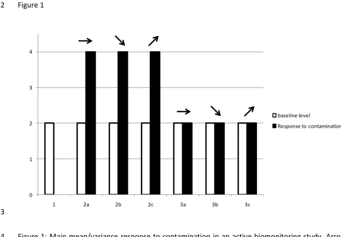
theoretical framework, we will develop three situations of mean variation (Fig. 1). 9

Case 1 is the simplest one: when facing contamination, all individuals die. Thus the diagnosis is easy, 10

the environment is toxic! Case 2 is the favorite of scientists and editors: a clear and indubitable 11

increase in mean is observed. Beyond the mean, the variance could also change, with the patterns 12

detailed in box 2. 13

Finally, case 3 is classically considered as a "no effect" response. However, while it's true for the 14

population 1a, the two others presented variation in variance, if not in mean. We must not neglect 15

this effect that could be the early warning signal that everybody is looking for. Indeed, the shift in 16

variance can occur before the shift in mean, though numerous case studies are needed to correctly 17

interpret such results. 18

19

Inter-population variability along environmental/pollution gradients

20

Passive biomonitoring cases are the most difficult to interpret, because they are the outcome 21

of a gene x environment interaction. By comparing several populations to a reference system, several 22

patterns could be observed. The values observed are not the responses to a change of environmental 23

10

condition, but the chronic, basal level of the studied parameter in the local environmental condition. 1

Thus, the objective is to understand whether the differences observed could be relevant indicators of 2

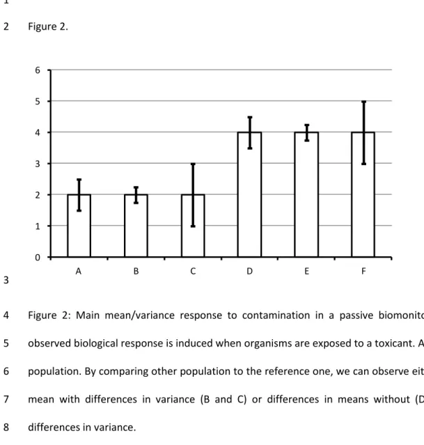
population health (Fig. 2). 3

The simplest result is the stability of both mean and variance that could be easily interpreted as the 4

absence of environmental stress. If no difference in mean is observed, while a difference in variance 5

exists (Fig 2., A vs B vs C), we can postulate that the chronic levels of contamination are similar 6

among the two studied sites. However, the phenotypic plasticity revealed by the response variability 7

tells about the genetic variability and the adaptative abilities of the population. It has been shown 8

that genetic variability is a key factor for population health, thus populations at risk are those with 9

the lowest variability. 10

The most complicated cases are those where several populations exhibit different mean levels of 11

their responses (A-B-C vs D-E-F). Indeed, without information on the temporal variation, we cannot 12

distinguish short term induction in response to a temporary stress or long term adaptation or 13

acclimatation to a chronic stress. In such situations, even the study of the variance is of no help. 14

Either temporal trends of the biological response or results of laboratory stress on stress 15

experiments would be helpful to understand these complex interactions. This leads us to question, in 16

an interpopulation perspective, the meaning of the basal level (in mean and variance), and how 17

useful it is to predict and interpret the response pattern. Such approaches are poorly developed. 18

They reveal within and between population phenotypic variability, that could be the outcome of 19

stochastic phenomenon (genetic drift or founder effect), but also the results of local adaptation 20

through selection by the contaminant pressure, or a simple acclimatation to local conditions. More 21

studies are necessary, either in the field or laboratory, to explore and understand the mechanisms 22

and the consequences of modification of variance patterns. 23

11

Towards the ecotoxicological niche: an ecological perspective to ecotoxicology

1

Information necessary to understand and exploit the different patterns of response within and 2

between populations relies on the natural variability, i.e. the range of values of the studied biological 3

response in a range of healthy ecosystems and for healthy populations, to correctly define the 4

baseline level (Xuereb et al. 2009; Coulaud et al. 2011; Lacaze et al. 2011; Jubeaux et al. 2012). 5

We can then define the ecotoxicological niche as the ability of species to cope with contamination 6

and to maintain basal physiological function when facing anthropogenic stress. This ecotoxicological 7

niche is thus a particular case of the traditional ecological niche, where the environmental gradient is 8

replaced by a chemical compound. Using this well known conceptual framework, we can adapt the 9

Shelford law (1931) and define a well-being zone (Figure 3), corresponding to the realized niche of a 10

population, a stress zone, corresponding to the potential niche, and a lethal zone, where acclimation 11

abilities are overwhelmed. 12

The main dimensions of this niche should be the classical ecotoxicological parameters related to 13

genetic and cellular damages, physiological and behavioral modifications, defense or exposure 14

system activation, but also more integrative parameters directly related to fitness (reproduction, 15

survival and growth). For each of these dimensions, the realized niche is defined as the inter-16

individual variability (95% confidence interval, for instance) observed in situ. To get a complete 17

overview of this realized niche, those parameters should at least be measured at several time scales, 18

depending on the life cycle of the species. The theoretical niche is not conceptually difficult to define, 19

as it should be drawn from the observation of several populations of the considered species, in 20

various environmental conditions (of pollution, geochemistry, hydromorphology…). Thus, it is just a 21

compilation of many realized niches. The most difficult parameter to evaluate is the potential niche, 22

which is the extreme deviation from the baseline that allows the population to maintain itself in the 23

ecosystem. This raises two problems: how to make sure that we measured the extreme deviation, 24

12

and how to ensure the sustainability of the population? It needs to combine an experimental and a 1

modeling approach. Experiments performed in realistic conditions (mesocosms), on long term to 2

allow acclimation phenomena, will be used to measure biological response levels. In the meantime, 3

population dynamics models based on the Dynamic Energy Budget in Toxicology (DEBtox) need to be 4

built to assess population sustainability (Billoir et al. 2007). The combination of those two 5

information will define the potential ecotoxicological niche defined above. 6

Once the three niche scales described, the population-level information (realized and potential) can 7

be compared to the species level information (theoretical niche), this comparison solving the 8

problem of interpopulation comparison, giving a general framework to interpret every response 9

observed. Indeed, if populations get different realized niches, but similar potential niches, we can 10

suppose that they are living in contrasted environments according to contamination. In the 11

meantime, if those differences in realized niche are small compared to the theoretical niche of the 12

species, we can suppose that the level of stress is far from the maximal level that they are able to 13

undergo. Finally, the potential niche breadth informs us on the sensitivity of each population to 14

stress. A next step should be to link ecotoxicological niche breadth to biological and ecological traits 15

such as feeding habits and food, maximum size, substrate preferences, trophic status (Poisot et al. 16

2011; Colas et al. 2014). 17

18

Consequences for Environmental Risk Assessment (ERA) approaches

19

The main objective of ERA approaches is to define the health status of a population. A frequent 20

confusion/debate is about the scale at which we should interpret biological responses measured on 21

an individual. We think that a misuse/misunderstanding is to consider that those parameters should 22

be interpreted as proxy of the individual health status. Well, they obviously reflect the individual 23

health status, but those individuals are sampled from a population, and thus also reflect the 24

13

population health status. Thus, individual-based measurements are population relevant indicators, 1

and as a consequence, variance between individuals should be interpreted as a populational 2

response. 3

Sacrifice complexity (and realism) on the altar of reproducibility

4

Biomarker approaches are often criticized for their lack of ecological relevance (McCarty et al 2002). 5

Indeed, to get fine information about the ecosystem health, a common approach is to focus on the 6

most sensitive species and on the most sensitive stages. However, finding such species looks like an 7

unattainable goal (Cairns Jr. 1992) and takes us away from a pertinent ecological risk assessment 8

(Baird and Barata 1999). In the same way, considering the spatio-temporal variability of physiological 9

status, the most sensitive stage at one time (which has been selected for ecotoxicology tests) could 10

be more resistant at another time (i.e. females should be more sensitive to lipophilic contaminants 11

before gestation than during). 12

Moreover, with the aim of controlling variability, ecotoxicology tests are based on a very specific 13

category of natural population. However, doing that, these tests are not suitable to build metric 14

representatives of the whole population. The response variability evidences phenotypic variants 15

within a population. For example, decreasing genetic diversity by selecting some clonal population of 16

Daphnia leads to an increase in uncertainty when performing field extrapolation (Barata et al. 2002).

17

Thus, with a limited, biased variability, we do not get a good idea of the adaptative possibilities 18

within the population, nor of the resilience/resistance abilities of the population. Therefore, rather 19

than minimize variability, it would be better to model the relative influence of intrinsic and extrinsic 20

factors on the studied biological response to better understand the system (Handy et al. 2003). 21

Finally, to demonstrate the effects of pollution and to predict population health, variance must 22

become a component of the evaluation scheme, as it can reflect system resistance and resilience 23

14

against perturbation (the assimilative capacity hypothesis (Cairns Jr. 1977, 1999; Death 2010; Steudel 1

et al. 2012)). 2

Acknowledgments

3

We want to thank Sharon Kruger for her linguistic corrections. This approach was developed within 4

the EC2CO Sydepop and ANR IPOC programs. We thank the reviewers whose comments helped us to 5

improve the manuscript. 6

References

7

Artigas J, Arts G, Babut M, Caracciolo AB, Charles S, Chaumot A, et al. Towards a renewed research 8

agenda in ecotoxicology. Environmental Pollution. 2012; 160: 201–6. 9

Baird DJ, Barata C. Genetic variation in the response of Daphnia to toxic substances: implications for 10

risk assessment. Genetics and ecotoxicology. Taylor and Francis. London: Forbes V.E.; 1999. 11

p. 207–21. 12

Barata C, Markich SJ, Baird DJ, Taylor G, Soares AMVM. Genetic variability in sublethal tolerance to 13

mixtures of cadmium and zinc in clones of Daphnia magna Straus. Aquatic Toxicology 2002; 14

60: 85–99. 15

Bard SM. Multixenobiotic resistance as a cellular defense mechanism in aquatic organisms. Aquatic 16

Toxicology. 2000 ;48: 357–89. 17

Bastos AC, Monaghan KA, Pestana JLT, Lillebø. AI, Loureiro S. A comment on the Editorial “Replication 18

in aquatic biology: The result is often pseudoreplication.”Aquatic Toxicology 2013; 126: 467-19

470 20

Beketov MA, Liess M. An indicator for effects of organic toxicants on lotic invertebrate communities: 21

independence of confounding environmental factors over an extensive river continuum. 22

Environmental Pollution. 2008; 156: 980–7. 23

Beketov MA, Speranza A, Liess M. Ultraviolet radiation increases sensitivity to pesticides: synergistic 24

effects on population growth rate of Daphnia magna at low concentrations. Bulletin of 25

environmental contamination and toxicology. 2011; 87: 231–7. 26

Bennett AF. Interindividual variability: an underutilized resource. New Directions in Ecological 27

Physiology. Cambridge University Press. Cambridge: Feder M.E., Bennett A.F., Burggren W.W. 28

and Huey R.B.; 1987. 29

Billoir E, Péry ARR, Charles S. Integrating the lethal and sublethal effects of toxic compounds into the 30

population dynamics of Daphnia magna: A combination of the DEBtox and matrix population 31

models. Ecological Modelling. 2007; 203: 204–14. 32

15

Browne R., Moller V, Forbes V., Depledge M. Estimating genetic and environmental components of 1

variance using sexual and clonal Artemia. Journal of Experimental Marine Biology and 2

Ecology. 2002; 267: 107–19. 3

Cairns Jr. Aquatic ecosystem assimilative capacity. Fisheries. 1977; 2: 5. 4

Cairns Jr. J. The threshold problem in ecotoxicology. Ecotoxicology. 1992; 1: 3–16. 5

Cairns Jr. J. Assimilative capacity — the key to sustainable use of the planet. Journal of Aquatic 6

Ecosystem Stress and Recovery. 1999; 6: 259–63. 7

Calow P. Variability: noise or information in ecotoxicology? Environmental Toxicology and 8

Pharmacology. 1996; 2: 121–3. 9

Colas F, Vigneron A, Felten V, Devin S. The contribution of a niche-based approach to ecological risk 10

assessment: Using macroinvertebrate species under multiple stressors. Environmental 11

Pollution. 2014; 185: 24–34. 12

Corton JC, Bushel PR, Fostel J, O’Lone RB. Sources of variance in baseline gene expression in the 13

rodent liver. Mutation Research - Genetic Toxicology and Environmental Mutagenesis. 2012; 14

746: 104–12. 15

Costantini D, Metcalfe NB, Monaghan P. Ecological processes in a hormetic framework. Ecology 16

Letters. 2010; 13:1435–47. 17

Coulaud R, Geffard O, Xuereb B, Lacaze E, Quéau H, Garric J, et al. In situ feeding assay with 18

Gammarus fossarum (Crustacea): Modelling the influence of confounding factors to improve

19

water quality biomonitoring. Water Research. 2011; 45:6417–29. 20

Death RG. Disturbance and riverine benthic communities: What has it contributed to general 21

ecological theory? River Research and Applications. 2010; 26: 15–25. 22

Depledge M. The rational basis for the use of biomarkers as ecotoxicological tools. In: Fossi M, 23

Leonzio C, editors. Nondestructive biomarkers in vertebrates. Lewis Publishers; 1994. p. 261– 24

85. 25

Depledge M.H., Lundebye A.K. Physiological Monitoring of Contaminant Effects in Individual Rock 26

Crabs, Hemigrapsus Edwardsi: The Ecotoxicological Significance of Variability in Response. 27

Comparative Biochemistry and Physiology -- Part C: Pharmacology, Toxicology and 28

Endocrinology. 1996; 113: 277–82. 29

Depledge MH. New approaches in ectoxicology: can inter-individual physiological variability be used 30

as a tool to investigate pollution effects? Ambio. 1990; 19: 251–2. 31

Depledge MH, Fossi MC. The role of biomarkers in environmental assessment (2). Invertebrates. 32

Ecotoxicology. 1994; 3: 161–72. 33

Drummond GB, Vowler SL. Variation: use it or misuse it – replication and its variants. Journal of 34

Physiology. 2012; 590: 2539–42. 35

16

Feckler A, Thielsch A, Schwenk K, Schulz R, Bundschuh M. Differences in the sensitivity among cryptic 1

lineages of the Gammarus fossarum complex. Science of The Total Environment. 2012; 439: 2

158–64. 3

Handy RD, Depledge MH. Physiological Responses: Their Measurement and Use as Environmental 4

Biomarkers in Ecotoxicology. Ecotoxicology. 1999; 8: 329–49. 5

Handy RD, Galloway TS, Depledge MH. A Proposal for the Use of Biomarkers for the Assessment of 6

Chronic Pollution and in Regulatory Toxicology. Ecotoxicology. 2003; 12: 331–43. 7

Hyne RV, Maher WA. Invertebrate biomarkers: links to toxicosis that predict population decline. 8

Ecotoxicology and Environmental Safety. 2003; 54: 366–74. 9

Jubeaux G, Simon R, Salvador A, Lopes C, Lacaze E, Queau H, et al. Vitellogenin-like protein 10

measurement in caged Gammarus fossarum males as a biomarker of endocrine disruptor 11

exposure: Inconclusive experience. Aquatic Toxicology 2012; 122: 9–18. 12

Karimi R, Folt CL. Beyond macronutrients: element variability and multielement stoichiometry in 13

freshwater invertebrates. Ecology Letters. 2006; 9: 1273–83. 14

Keppler C, Ringwood AH. Expression of P-glycoprotein in the gills of oysters, Crassostrea virginica: 15

seasonal and pollutant related effects. Aquatic Toxicology. 2001; 54: 195–204. 16

Knillmann S, Stampfli NC, Noskov YA, Beketov MA, Liess M. Elevated temperature prolongs long-term 17

effects of a pesticide on Daphnia spp. due to altered competition in zooplankton 18

communities. Global Change Biology. 2103; 19: 1598-1609. 19

Lacaze E, Devaux A, Mons R, Bony S, Garric J, Geffard A, et al. DNA damage in caged Gammarus 20

fossarum amphipods: A tool for freshwater genotoxicity assessment. Environmental

21

Pollution. 2011; 159: 1682–91. 22

Lazic S. The problem of pseudoreplication in neuroscientific studies: is it affecting your analysis? BMC 23

Neuroscience. 2010; 11: 5. 24

Luoma SN. The developing framework of marine ecotoxicology: Pollutants as a variable in marine 25

ecosystems? Journal of Experimental Marine Biology and Ecology. 1996; 200: 29–55. 26

Maul A. Heterogeneity: A Major Factor Influencing Microbial Exposure and Risk Assessment. Risk 27

Analysis. 2014; In press : DOI: 10.1111/risa.12184. 28

Minguez L, Buronfosse T, Beisel J-N, Giambérini L. Parasitism can be a confounding factor in assessing 29

the response of zebra mussels to water contamination. Environmental Pollution. 2012; 162: 30

234–40. 31

Morgan AJ, Kille P, Stürzenbaum SR. Microevolution and Ecotoxicology of Metals in Invertebrates. 32

Environmental Science and Technology 2007; 41: 1085–96. 33

Nikinmaa M, Tjeerdema R. Environmental variations and toxicological responses. Aquatic Toxicology. 34

2013; 127: 1. 35

Nikinmaa M., Celander M., Tjeerdema R. Replication in aquatic biology: The result is often 36

pseudoreplication. Aquatic Toxicology. 2012; 116-117: iii–iv. 37

17

Odum EP, Finn JT, Franz EH. Perturbation Theory and the Subsidy-Stress Gradient. BioScience. 1979; 1

29: 349–52. 2

Poisot T, Bever JD, Nemri A, Thrall PH, Hochberg ME. A conceptual framework for the evolution of 3

ecological specialisation. Ecology Letters. 2011; 14: 841–51. 4

Smith R, Mann R, Fox D. Variability in ecotoxicology: deliberate ignorance or just not getting it. 6th 5

SETAC World Congress / SETAC Europe 22nd Annual Meeting , Berlin, Germany; 2012. 6

Steinberg CEW, Stürzenbaum SR, Menzel R. Genes and environment — Striking the fine balance 7

between sophisticated biomonitoring and true functional environmental genomics. Science 8

of The Total Environment. 2008; 400: 142–61. 9

Steudel B, Hector A, Friedl T, Löfke C, Lorenz M, Wesche M, et al. Biodiversity effects on ecosystem 10

functioning change along environmental stress gradients. Ecology Letters. 2012; 15: 1397– 11

405. 12

Violle C, Enquist BJ, McGill BJ, Jiang L, Albert CH, Hulshof C, et al. The return of the variance: 13

intraspecific variability in community ecology. Trends in Ecology & Evolution. 2012; 27: 244– 14

52. 15

Williams TD. Individual variation in endocrine systems: moving beyond the “tyranny of the Golden 16

Mean.”Philosophical Transactions of the Royal Society – Biological Sciences. 2008; 363: 17

1687–98. 18

Xuereb B, Chaumot A, Mons R, Garric J, Geffard O. Acetylcholinesterase activity in Gammarus 19

fossarum (Crustacea Amphipoda): Intrinsic variability, reference levels, and a reliable tool for

20

field surveys. Aquatic Toxicology. 2009; 93: 225–33. 21 22 23 24 25 26 27 28 29 30

18

Box 1: experimental design (for recent review and analysis of pseudoreplication, see(Bastos et al.; 1

Lazic 2010; Drummond and Vowler 2012; Nikinmaa M. et al. 2012). 2

5 « independant » experimental units per condition

1 measure per unit

= 5 replicates

If you focus on mean, the good practice is :

Condition A Condition B

1 experimental units per condition

5 measure per unit

= 5 pseudoreplicates

BUT if you focus on variance, the good practice is :

Condition A Condition B

Replicated samples take into account two sources of variability : experimental units differences and inter-individual differences. Pseudo-replicated samples only consider the variability within population. The best way is to mix the two methods, that allows to work on the mean and on the variance.

3 4

19 1

Box 2 :Intra-population variance scenarios 2

CL10 CL50

sublethal

lethal

sublethal

lethal

sublethal lethal

(a)

(b)

(c)

(d)

(e)

The case considered is an increase of the measured parameter in response to contamination. Beside the mean, several trends in the variance could be observed.

Sublethal exposure. The variance could be constant across conditions (a), revealing a

low phenotypic variability, probably associated to a low genetic variability. A decrease in variance (b), often associated to a high variability of basal levels, could be interpreted as a canalization of the response to the most efficient one. Finally, the variance could increase (c). This last case could be linked to a continuous variation of the response in the interval observed, or to the constitution of several distinct groups of individuals (low, intermediate and high values for instance). Thus this high variability at concentrations near the lethality threshold is linked to individuals that exhibit extreme values, reflecting either low resistance abilities or a risk for the biological responses to be overcome (i.e. once the highest possible value is attained, health impairments are expected). Those two extreme situations can lead to death if the stress is maintained.

Lethal exposure. Over the lethality threshold, a decrease in variance indicates that all

individuals displaying extreme values are dead. If the mean decreases (d), we can suppose that individuals exhibiting the highest responses are dead and that high induction is a signal of a soon overcoming of regulation/defense system. The last case (e) is an increase of the mean, indicating that low values of the response are linked to insufficient induction and an inability of individuals to protect themselves.

3 4

20 1 Figure 1 2 0 1 2 3 4 1 2a 2b 2c 3a 3b 3c baseline level Response to contamination 3

Figure 1: Main mean/variance response to contamination in an active biomonitoring study. Arrows 4

indicates the direction of variance changes. 5

21 1 Figure 2. 2 0 1 2 3 4 5 6 A B C D E F 3

Figure 2: Main mean/variance response to contamination in a passive biomonitoring study. The 4

observed biological response is induced when organisms are exposed to a toxicant. A is the reference 5

population. By comparing other population to the reference one, we can observe either a stability of 6

mean with differences in variance (B and C) or differences in means without (D) or with (E, F) 7

differences in variance. 8

22 1

Well-Being

Realized niche

inhibition induction

Potential niche breadth

Str

es

s

Lethal

Lethal

Ecotoxicological niche

P

o

p

u

la

ti

o

n

s

iz

e

extinction

treshold

Str

es

s

Figure 3: The ecotoxicological niche. The optimal health status for a given population is attained for 3

its realized niche, i.e.when the natural, chronic conditions are encountered, contamination included. 4

This niche thus encompasses acclimation and adaptation phenomenon. The presence of a 5

supplementary contamination represents an important deviation from these standard conditions, 6

leading to an increase or a decrease of the biological response, depending on the parameter 7

considered. A first level still allows the population to maintain itself, with lower abundances: it's the 8

potential niche. Then this potential niche is overcome, the environment became too far from the 9

adaptative abilities of the population, which lead to local extinction. 10