HAL Id: hal-01093631
https://hal.archives-ouvertes.fr/hal-01093631
Preprint submitted on 10 Dec 2014
HAL is a multi-disciplinary open access
archive for the deposit and dissemination of sci-entific research documents, whether they are pub-lished or not. The documents may come from teaching and research institutions in France or abroad, or from public or private research centers.
L’archive ouverte pluridisciplinaire HAL, est destinée au dépôt et à la diffusion de documents scientifiques de niveau recherche, publiés ou non, émanant des établissements d’enseignement et de recherche français ou étrangers, des laboratoires publics ou privés.
Commodity returns co-movements: Fundamentals or
”style” effect?
Philippe Charlot, Olivier Darné, Zakaria Moussa
To cite this version:
Philippe Charlot, Olivier Darné, Zakaria Moussa. Commodity returns co-movements: Fundamentals or ”style” effect?. 2014. �hal-01093631�
EA 4272
Commodity returns co-movements:
Fundamentals or “style” effect?
Philippe Charlot*
Olivier Darné*
Zakaria Moussa*
2014/30
(*) LEMNA, Université de Nantes
Laboratoire d’Economie et de Management Nantes-Atlantique Université de Nantes
Chemin de la Censive du Tertre – BP 52231 44322 Nantes cedex 3 – France
www.univ-nantes.fr/iemn-iae/recherche
D
o
cu
m
en
t
d
e
T
ra
va
il
W
o
rk
in
g
P
ap
er
Commodity returns co-movements: Fundamentals or “style”
effect?
Philippe Charlot∗ Olivier Darné† Zakaria Moussa‡§
Abstract
This paper investigates dynamic correlations both across commodities and between commodities and traditional assets, such as equities and government bonds, using the Regime Switching Dynamic Correlation (RSDC) model. In particular, this paper assesses the dynamics of 32 daily commodity futures returns, spanning a period from May 28, 2003, to June 04, 2014, in the light of economic and financial events before and after the mid-2007 financial crisis. There are three major findings. First, prior to the financial crisis, we detect stronger correlation among the wide range of commodities used in the analysis, indicating that the financialization process started impacting commodity price movements from mid-2005. Between commodities taken as an asset class and traditional asset classes our results generally show very weak commodity-equity and commodity-bond correlations prior to the Lehman Brother collapse. This can be explained by the “style ”effect theory that correlations between different asset classes in a portfolio weaken. Second, during the financial crisis, correlations both across commodities and between commodities and equities increase dramatically, with a regime change which coincides exactly with the demise of Lehman Brothers on September 15, 2008. This suggests that a strong commodity-equity integration was temporarily masked by the “style ”effect. However, commodity-bond correlations switch to a strongly negative regime, showing that government bonds were considered as refuge securities. Third and most importantly, the new and original finding here is the temporary nature of the financial crisis effect identified, as correlations both across commodities and between commodities and traditional assets revert to pre-crisis level from April 2013. This highlights the impact of the financial-based factors on commodity price movements.
JEL classification: C22; G01; G10; G12; Q4
Keywords: Financialization; Style effect; Commodities; Cross-market linkages; Financial crisis; RSDC model
∗LEMNA, University of Nantes, France, [email protected] †LEMNA, University of Nantes, France, [email protected]
‡Corresponding author. LEMNA, University of Nantes, France, [email protected].
§This study is supported by the Chair Finance of the University of Nantes Research Foundation. We would
like to thank participants at the seminar of Banque de France and the 31st Spring International Conference of the French Finance Association for their valuable feedback.
1
Introduction
The most attractive aspect of commodity investments is that they offer diversification benefits both by hedging against inflation and by improving the risk-adjusted performance of a mixed-asset portfolio due to the low, or even negative, correlations between this alternative class of assets and traditional assets, such as equities or bonds (Gorton and Rouwenhorst, 2006;Chong and Miffre, 2010; Daskalaki and Skiadopoulos, 2011; Büyükşahin et al., 2010; Büyükşahin and Robe,2014). As equities performed poorly for two years following the 2000 burst of the Internet bubble, these alternative assets were therefore increasingly included in the strategic portfolio allocation process by institutional investors, particularly pension funds.
Investable commodity indices offer wide exposure to different commodity futures in differ-ent sectors of commodity markets, allowing index investors to reduce the risk of their overall investment portfolios whilst avoiding the problems involved in managing the physical goods. Commodity index swap dealers, having short positions with their investors, must hedge their positions by taking long positions on the underlying commodity futures. The inflow of index investors initiates the commodity financialization process1.
Before the 2007-2008 financial crisis, decreases in equity prices were generally accompanied by increases in commodity prices, reflecting a certain autonomy between commodity and equity markets. A new feature that emerged from the recent financial crisis was similar trends in equity and commodity markets. The synchronized sharp decline in equity and commodity prices in 2008 indicates increasing correlations between the two markets. Tang and Xiong (2010, 2012) stressed the importance of financialization in increasing the correlation both amongst seemingly unrelated commodities and between commodity and equity returns; the financial crisis simply further magnified this effect. This raises the question of the role of commodities as a diversification tool. The aim of this paper is twofold. Firstly, we analyze correlations both across commodity futures and between commodity futures and traditional assets, focusing on commodity-equity correlation. Secondly, we measure the impact of the 2007-2008 financial crisis, assessing whether the crisis caused a temporary or a permanent shift in the correlation trend, thereby providing insights into commodity price movements during recent years.
Existing theories on correlations across indexed assets show how fundamentally uncorrelated assets may move together when they become index constituents. According to the “style invest-ment”theory of Barberis and Shleifer (2003) and Barberis et al. (2005), constructed for stock markets and adapted by Basak and Pavlova (2013) to commodities, commodity index invest-ment increases correlations among seemingly unrelated commodities in commodity index. This increases homogeneity among indexed commodities, leading them to be accepted as a distinct asset class or “style”, like equity and fixed interest asset classes. However, commodity index in-vestments may have two counteracting effects on co-movements between commodity indices, and therefore on index constituents and traditional assets like stocks, depending on index investors’ rebalancing strategies and the composition of their portfolios. On the one hand, commodity index trading can act as a channel leading to higher correlations with other assets in a portfolio. As index investors, having incentives to maintain their portfolio diversification level, rebalance their portfolios between commodities and stocks when a shock alters portfolio weights, correlations among the different assets increase (Basak and Pavlova(2013)). On the other hand, to be rec-ognized as an asset class, commodity futures need to exhibit a sufficiently low correlation with
1
The World Bank estimates as much as $325 billion worth of assets are under the management of the hedge fund industry, about nine times higher than in the last decade (World Bank Commodity Market outlook 2012,...2014). Moreover, the total amount invested in commodity derivatives in the over-the-counter market of securities firms or banks of the leading 11 developed countries rapidly increased after 2005 from $1400 trillion (base for notional value) in December 2004 to $ 9000 trillion in December 2007 (BIS, Regular OTC Derivatives Market). Also, a CFTC staff report (2008) estimates that the total amount invested in commodity indices by non-commercial participants increased from $15 billion in 2003 to $200 billion in 2008.
other asset classes; this is one of the qualitative criteria (in addition to sufficient market capital-ization, availability of pricing and investability). Barberis and Shleifer(2003) consider this weak correlation as a consequence of the "style" competition caused by the externality generated by switcher investors: switching portfolio composition between commodity indices and stocks leads to a weak, even negative, correlation between the two competing asset classes. To sum up, index investments can have a positive as well as a negative impact on commodity-equity correlations, the overall co-movement reaction depending on whether positive or negative effects prevail.
However, in times of financial crisis, regardless of these theoretical index investment effects, correlations may sharply increase between different asset classes included in investors’ portfolios, particularly between commodities and equities, the largest part of investors’ portfolios (Kyle and Xiong, 2001; Brunnermeier and Pedersen, 2009). When a market collapses, investors, particu-larly leveraged, are drawn into a "loss spiral" (Brunnermeier and Pedersen(2009)) and sell risky assets to raise liquidity, causing falls in unrelated asset returns.2 Although again unrelated to fundamentals, this common effect sharply increases correlations, both across commodities as a distinct asset class and between commodities and other asset classes. This is in line with the
Büyükşahin et al. (2010) notion of a “market of one”, postulating an increase in co-movements among unrelated asset classes during turbulent periods. Relatedly,Singleton(2012) documents a significant contribution by flows from institutional investors to the 2008 boom/bust in oil prices. Numerous empirical studies examine the link between commodity and equity markets before the financial crisis. There seems to be broad consensus that correlations between these two assets are weak and generally follow a decreasing trend, suggesting that commodity futures do improve diversification benefits for investors. Jensen et al. (2000) and Erb and Harvey (2006) report that the correlation between commodity futures returns and the S&P 500 is weak and even negative for some commodities. Chong and Miffre (2010) apply the multivariate dynamic conditional correlation (DCC) GARCH approach introduced byEngle (2002) on 25 commodities and seven equity assets (within the S&P 500 index), spanning the period from December 12, 1980 to December 27, 2006. They find that the conditional correlations between commodity and S&P500 returns fall over time, a sign that commodity futures have become better tools for strategic asset allocation. Conversely,Choi and Hammoudeh(2010) study the correlation between five commodities (Brent oil, WTI oil, copper, gold and silver) and the S&P 500 index, using the DCC GARCH model, for the period between January 2, 1990 and May 1, 2006. Their results show that equity-commodity correlations started to rise as early as 2003 and hence diversification benefits declined.
Büyükşahin et al. (2010) study the correlation between the S&P 500 and six commodity sub-indices, namely, Agriculture, Energy, Industrial Metals, Livestock, Non-Energy and Precious Metals. They treat structural breaks exogenously by using subsample analysis for the periods June 1991-May 1997, June 1997-May 2003 and June 2003-November 2008. They contend that, even though the co-movements between equities and commodities increased substantially during the financial crisis, they remained lower than their peaks in the previous decade, suggesting that commodities retained their role as a diversification tool. These findings are consistent with those inBüyükşahin and Robe(2014) using updated data from January 1991 to February 2010.
In order to take into account correlation regime changes,Silvennoinen and Thorp(2013) apply a bivariate conditional volatility and correlation dynamics model (DSTCC-GARCH), developed by Silvennoinen and Teräsvirta (2009). They include 24 individual commodity futures returns along with major equity indices in the U.S. and Europe from May 1990 to July 2009, plus US government bonds, and use either time calendar or the implied volatility index (VIX) as transition variables governing the correlation switch. Contrary to Büyükşahin et al. (2010), Büyükşahin and Robe (2014) and Chong and Miffre (2010), their main findings are in line with those of
2
Closely related to the "loss spiral" theory ofBrunnermeier and Pedersen(2009),Kyle and Xiong(2001) propose a model explaining that in times of financial crisis, financial intermediaries experience wealth effects reducing their risk-bearing capacity and pushing them to sell all types of assets held in their portfolios.
Tang and Xiong(2010,2012). They support the rising trend hypothesis, i.e. that all commodity correlations with stock indices, except for gold, start to increase gradually well before the financial crisis, reflecting the effect of financial integration between markets, and grow sharply during the turbulent period of the financial crisis. However, correlation with the bond market is generally weak and constant over the sample data, being particularly low, or even switching to a negative regime, for Industrial Metals.
Our paper contributes to this rich debate by extending previous studies in two principal re-spects. First, from a methodological perspective, a novel and distinctive feature of the paper is that it adopts the Regime Switching for Dynamic Correlations (RSDC) model ofPelletier(2006), estimated using the EM (Expectation–Maximization) algorithm. Both in DSTCC, applied by
Silvennoinen and Thorp (2013), and in RSDC, dynamic correlations can switch between two or more constant correlation matrices, depending on the number of regimes. The main difference between the two approaches lies in the assumption concerning the mechanism that governs the switch. The DSTCC assumes a deterministic switch based on a conditional transition function which includes smoothing and localization parameters and either deterministic or stochastic tran-sition variables. The problem with such an approach is that the regime switch depends on the transition variable selected. This problem does not arise with the RSDC, however, as it assumes that the switch between constant correlation matrices is established through an underlying hid-den stochastic process with a first order Markov chain. Moreover, the DSTCC model encounters major numerical problems when estimated with a large number of series, whereas the RSDC can be applied to a large dataset, especially when it is estimated using an EM algorithm. The ease with which the RSDC performs large-scale estimations allows us to model series in groups, whereas the DSTCC would only be able to deal with bivariate estimations. Second, applying the EM algorithm to estimate the model allows us to exploit a more extensive data set, covering the period of the 2007-2008 financial crisis. While most papers use either commodity indices or a few individual commodity futures prices, we consider daily data for the four major commodity indices and 32 individual commodity futures returns, along with stock and bond returns, span-ning a period from May 28, 2003, to June 04, 2014. Our sample period allows for analysis to be performed before and after the financialization as well as during the financial crisis and the subsequent changes, so as to clearly distinguish between financialization-related and crisis-related effects on the change in correlation trend.
Our main findings can be summarized as follows. First, before the financial crisis, our results confirm the theoretical findings of both “style effect”and asset management allocation: we detect stronger integration among the large selection of commodities used in the analysis. Moreover, as inTang and Xiong(2010,2012), we find that correlations between Non-Energy commodities and WTI started to increase well before the recent financial crisis, indicating that the financializa-tion process started impacting commodity price movements prior to the recent turbulent period. However, regarding correlations between commodities as an asset class and traditional financial assets, our results generally show very weak commodity-equity and commodity-bond correlations prior to the Lehman Brothers collapse. This proves the relevance of the “style effect”theory to explain the dynamic links between commodities and both stock and bond markets. However, it may not be possible to consider commodities as a fully-fledged “style”, as we detect a significant heterogeneity among commodity groups. Our second major finding is that, during the financial crisis, correlations both across commodities and between commodities and equities increased dra-matically, with a regime change that coincided perfectly with the demise of Lehman Brothers on September 15, 2008. This reflects the “loss spiral”effects during the period of financial market tensions. However, commodity-bond correlations switched to a strongly negative regime, showing that government bonds were being considered as refuge securities. The third and most important of our findings contributes to the debate by revealing the temporary nature of the financial crisis effect. Correlations both across commodities and between commodities and traditional assets re-verted to their pre-crisis level by April 2013, thus confirming that financial-based factors impact
commodity price movements.
In the next section, we outline the econometric methodology used in the empirical analysis. Section 3 presents detailed descriptive statistics of the dataset. Section 4 discusses empirical results of analysis across commodities. Section 5 focuses on correlations between commodities and traditional assets. Section 6 concludes.
2
Methodology
In this paper, we adopt the general framework of multivariate GARCH models with dynamic conditional correlations. Introduced byBollerslev (1990), the conditional correlations model was finely tuned by Engle and Sheppard (2001) to introduce time-varying conditional correlations. Formally, the general framework of multivariate GARCH models with dynamic correlations as-sumes that a stochastic process rt of size (K × T ) is defined by:
rt|Ft−1∼ L(0, Ht) (1)
where Ft−1 refers to the information set generated by the observed series rt up to t − 1, while L is a distribution function with zero mean and conditional variance Ht. The expression of Ht is given by: Ht= DtRtDt (2) where: Dt= diag(h1/21,t , ..., h 1/2 K,t) (3)
is a diagonal matrix composed of the standard deviation of the K univariate series. This
de-garching tranformation leads to expressing the standardized residuals as:
ǫt= D−1t rt (4)
Then, the expectation of the standardized residuals gives the conditional correlations.
The seminal specification of Engle and Sheppard (2001) proposes a time-varying conditional correlation using an autoregressive formulation for Rtsuch that:
Rt= diag {Qt}−1/2Qtdiag {Qt}−1/2 (5)
The conditional covariance matrix Qt is expressed as a BEKK formulation:
Qt= (1 − α − β)Q + αǫi,t−kǫ′j,t−k+ βQt−l (6)
in which Q is the unconditional covariance matrix. Enthusiasm for this class of models resulted in a vast literature, as exhaustively reviewed byBauwens et al.(2006),Silvennoinen and Teräsvirta
(2009),Engle (2009) and Francq and Zakoian(2010).
In this paper, we study the conditional correlations given two constraints arising from our dataset: computationally feasible estimation of the model and the possibility of breaks. A few Markov-switching models have been proposed, like Billio and Caporin (2005), Pelletier (2006) andHaas and Mittnik(2008). The advantage of the Regime Switching for Dynamic Correlations (RSDC) model ofPelletier(2006) lies in offering a Markov-Switching structure for the correlation process by imposing constant correlations within each regime but switch from one regime to another via a Markov chain of order one, at the same time as making it possible to estimate with large datasets. The RSDC model assumes that the conditional correlation matrix has the form:
Rt= N Ø n=1 1{sn=i}Rn (7) 5
where {st}t∈Nis a first order Markov chain with N states and Rn a constant correlation matrix. In other words, the correlations evolve between N constant correlations matrices, moving from one to another according to the Markov chain.
The first advantage of the RSDC is economic: unlike autoregressive formulations, which are difficult to understand from an economic point of view, this model has a clear cut economic ex-planation because each regime is linked to a constant correlation matrix. Secondly, this model can be estimated using an EM algorithm. In fact, the drawback of many dynamic conditional correlations models lies in the fact that estimation of parameters for large datasets can encounter difficulties in handling extensive data. Being able to apply an EM algorithm means that less structured models do not need to be used when handling large datasets.
We use a two-stage estimation for the RSDC where the log- likelihood is written as the sum of the volatility component and the correlation term. For the first step, we perform the estima-tion of each univariate volatility model using a search procedure across a class of 8 univariate GARCH specifications selected according to the Bayesian information criterion (BIC). Finally, log-likelihood of the volatility component can be written as:
L(θ1) = − 1 2 T Ø t=1 ! Klog(2π) + log(|Dt|2) + yt′Dt−2yt" (8) where θ1 denotes the parameter space for the univariate volatility. The log-likelihood of the correlation term is expressed as follows:
L( ˆθ1, θ2) = − 1 2 T Ø t=1 ! log(|Rt|) + ε′tR−1t εt− ε′tεt" (9) with θ2 the parameter space for the correlation part. Because the latent process is unobserved, the estimation step requires inferring the state of the Markov chain. Let ξjt be the probability of being in regime j given the information set available at time t − 1 and ηjt the density under regime j. The probability ˆξt|t of being in a regime at time t given the observations up to t can be computed using Hamilton’s filter:
ˆ ξt|t= ( ˆξt|t−1◦ ηt) 1′( ˆξt|t−1◦ ηt) (10) with: ˆ ξt|t+1= P × ˆξt|t (11)
where P is a transition matrix and ◦ denotes the element-by-element multiplication. Based on
Hamilton(1994), the re-estimation formula allows the elements pij of the transition matrix P to be updated: ˆ pij = qT t=2P(st= j, st−1= i|εT, ˆθ2) qT t=2P(st= i|εT, ˆθ2) (12) There is no re-estimation formula for directly updating the correlations matrices. In a first step, we update the covariance matrices Qn of the standardized residuals:
ˆ Qn= qT t=1(ˆεtεˆ′t)P(st= n|εT, ˆθ2) qT t=1P(st= n|εT, ˆθ2) (13) and then obtain the correlations matrices ˆRn by rescaling the covariance ˆQn using the transfor-mation defined in equation 5. As noted by Pelletier (2006), this rescaling produces a value for the log-likelihood obtained by the EM algorithm that does not exactly match the value computed with a Newton-type algorithm, but remains very close to it. Nonetheless, the EM algorithm al-lows very rapid estimation of high-dimensional systems while maintaining a full structured model where models estimated with numerical methods fail.
3
Data
3.1 Descriptive statistics
The data considered in this study consist of 4 commodity indices, namely, the S&P Goldman Sachs Commodity Index (GSCI), the Dow-Jones UBS (DJ-UBS) Commodity Index (which are the dominant commodity benchmarks for investors) the Rogers International Commodity index (RICI) and the Thomson Reuters/Jefferis CRB Index (CRB), as well as 32 individual commodity futures contract price series. The traditional assets include the S&P500 as equity asset index and JP Morgan US Government Bond total returns (JPMUS) as bond assets, along with a measure of volatility, the CBOE VIX volatility index, also considered a fear index on financial markets.3 Frequency is daily from May 28, 2003, to June 4, 2014, for a total of 2876 observations. Futures contract series can be classified in groups, representing various sectors of the commodity market, as follows:
1. Energy: crude oil (WTI), coal, natural gas.
2. Precious Metals: gold, silver, palladium, platinum.
3. Industrial Metals: aluminum, copper, zinc, tin, lead, nickel.
4. Agriculture: barley, corn, oats, rice, soybeans, soybean oil, wheat, palm oil, sunflowers, cocoa, coffee, sugar, cotton, lumber and orange juice.
• Grains: barley, corn, oats, rice, soybeans, wheat and sunflowers. • Softs: cocoa, coffee, sugar, cotton, lumber and orange juice. 5. Livestock: live cattle, lean hogs, feeder cattle.
Commodity futures prices used in this study are from Bloomberg, which provides what is known as “generic”futures. Many factors need to be considered in computing “generic”or contin-uous contracts in order to avoid significant price jumps or drops when concatenating contracts for the same commodity over time. Bloomberg builds “generic”futures series by using a nearest futures contract approach, rolling over from the most active contract or the contract nearest to expiry to the next nearest one. The active contract is typically based on the open interest and volume in the contract.4 Our empirical work uses a data set where all variables have been transformed to returns by multiplying the first difference of the logarithm by 100. In order to approximate the true cost as closely as possible and following Silvennoinen and Thorp (2013) andHong and Yogo(2011), we take an equally weighted average across returns to generic futures with the available maturity dates in each period and collateralize with the 3-month US Treasury Bill (T-bill), as the risk-free rate, as follows: yit,F = K1 qKk=1råi,t,τk + rf,t, where åri,t,τk is the log
return to k-th futures contract with maturity τk, and rf is the daily T-bill rate.
Tables1and 2report the summary statistics for different asset classes. As reported in earlier studies, commodity indices and commodity futures other than natural gas and aluminum have higher mean daily returns, between 3% and 6%, than those of traditional assets, about 2% and 0.25% for S&P 500 and Bonds, respectively. These high commodity returns are coupled with higher volatility relative to both equity and bond assets, confirming the commonly-observed excessive commodity price volatility over recent years attributed to either the boom-and-bust cycle or to excessive speculation by index investors.5 Furthermore, all series are leptokurtotic,
3
Data details and sources are given in the Dataset Appendix.
4
More details about generic contracts are given inChantziara and Skiadopoulos(2008).
5
For more details about the two opposing explanation for excessive commodity price volatility, seeTang and Xiong(2010,2012).
Table 1: Descriptive statistics: commodity futures returns.
Mean∗ Min Max Var. S. dev. Med. Kurtosis Skewness Engle LM test∗∗
wti 0.0438 -8.9974 9.8897 3.0802 1.7550 0.0610 6.4176 -0.1863 10.6053 (5.9791e−02) heating oil 0.0469 -8.6200 8.5821 2.7989 1.6730 0.0090 5.2767 -0.0761 9.8504 (7.9586e−02) natural gas -0.0148 -10.5418 8.3090 3.3323 1.8255 0.0148 4.6865 0.0976 22.7141 (3.8280e−04) coal 0.0209 -9.8928 10.3161 1.7355 1.3174 -0.0209 13.2462 -0.3336 35.1850 (1.3820e−06) gold 0.0423 -9.9038 7.8360 1.4245 1.1935 0.0043 8.1521 -0.5370 3.1449 (6.7766e−01) silver 0.0413 -17.7329 12.6415 3.9884 1.9971 0.0647 9.1641 -0.7097 2.5285 (7.7220e−01) platinum 0.0301 -7.1475 11.4117 1.3411 1.1581 0.0210 10.1054 0.0579 9.6109 (8.7043e−02) palladium 0.0500 -13.0528 9.8420 4.1915 2.0473 0.0067 6.6506 -0.5696 11.7640 (3.8168e−02) aluminum 0.0100 -7.7585 5.6434 1.8475 1.3592 -0.0039 5.2381 -0.3544 6.6848 (2.4516e−01) copper 0.0474 -10.1199 11.5452 3.3368 1.8267 -0.0288 6.7288 -0.1615 10.4875 (6.2545e−02) nickel 0.0280 -15.6456 12.8105 5.5945 2.3653 -0.0279 6.1572 -0.1705 3.5365 (6.1787e−01) lead 0.0520 -12.8007 12.3169 4.7691 2.1838 0.0189 6.0628 -0.2894 4.4848 (4.8191e−01) tin 0.0547 -11.0386 13.7926 3.6308 1.9055 0.0033 7.9563 -0.2254 5.7381 (3.3254e−01) zinc 0.0326 -10.2372 8.3663 3.9190 1.9796 -0.0092 5.2176 -0.2584 5.0592 (4.0870e−01) corn 0.0224 -7.3758 8.7767 2.1265 1.4583 -0.0200 5.9026 -0.0074 1.6067 (9.0044e−01) soybeans 0.0274 -7.1534 6.6567 2.3152 1.5216 0.0345 5.5978 -0.3652 1.6498 (8.9516e−01) soybean oil 0.0198 -7.0416 6.5350 2.0287 1.4243 -0.0165 5.3922 -0.0027 1.8563 (8.6865e−01) wheat 0.0243 -8.2315 7.2575 2.4635 1.5696 -0.0231 5.5793 -0.0184 6.8854 (2.2930e−01) coffee 0.0324 -10.7111 10.9987 3.1794 1.7831 -0.0099 5.5894 0.1429 6.1642 (2.9057e−01) cotton 0.0093 -7.8303 6.2534 1.9679 1.4028 0.0230 5.2593 -0.1629 6.4381 (2.6589e−01) orange juice 0.0201 -11.3623 10.2091 2.7022 1.6438 0.0295 7.1633 -0.2721 9.2091 (1.0101e−01) barley 0.0112 -54.5683 53.4137 5.5580 2.3575 -0.0112 212.7716 0.4454 11.4333 (4.3435e−02) oats 0.0289 -11.1912 11.8538 2.6695 1.6339 0.0096 7.6775 -0.0651 18.6134 (2.2682e−03) rice 0.0205 -6.7346 6.3782 1.6521 1.2853 -0.0205 4.8653 0.0047 4.9306 (4.2441e−01) palm oil 0.0202 -10.0779 7.4185 1.7139 1.3092 -0.0198 8.6608 -0.4479 2.3458 (7.9952e−01) cocoa 0.0235 -8.8601 7.5449 2.6824 1.6378 -0.0067 5.8077 -0.1880 3.7737 (5.8244e−01) sugar 0.0297 -10.4868 6.7202 2.3486 1.5325 0.0116 7.4521 -0.6231 12.5627 (2.7840e−02) lumber 0.0079 -5.1275 7.0852 1.3683 1.1697 -0.0079 5.4558 0.4772 17.9320 (3.0329e−03) sunflowers 0.0321 -8.2065 12.6384 0.7954 0.8919 -0.0265 23.0523 0.2749 111.0000 (0.0000e+00) lean hogs 0.0180 -4.9718 5.9656 0.8693 0.9324 0.0344 5.6446 -0.2404 1.7156 (8.8693e−01) live cattle 0.0233 -4.0081 3.2186 0.4796 0.6925 0.0150 5.7203 -0.3185 6.1628 (2.9070e−01) feeder cattle 0.0287 -4.9763 3.0858 0.4940 0.7029 0.0076 5.8747 -0.3607 18.9979 (1.9238e−03) Engle DCC test∗∗ (118.7318) (0.0000e+00)
In brackets, critical values for the tests.∗Mean of the series in returns.∗∗With 5 lags.
This table reports summary statistics for the 32 daily collateralized commodity futures returns from May 28, 2003 to June 4, 2014. We take futures returns (changes in log prices multiplied by 100) and collateralize them with the daily 3-month US Treasury Bill (T-bill) secondary market rate. Details about commodity futures contracts and sources are provided in Appendix A.
with some high values for barley and sunflowers. One explanation for the increasing demand for commodities in recent years is return distribution. As commodity returns are usually positively skewed and less volatile than traditional assets, which are usually positively skewed, they entail lower downward risk than traditional assets. When the tail event occurs simultaneously for both commodities and traditional assets, commodities add diversification benefits to the portfolio allocation. Conversely, however, for the considered sample, the distribution of commodity returns is negatively skewed, except for natural gas, barley, soybean oil, sunflowers and lumber, also showing volatility relative to traditional assets, suggesting that the diversification benefits of commodities can vanish.
Table 2: Descriptive statistics: commodity indices and financial series.
Mean∗ Min Max Var. S. dev. Med. Kurtosis Skewness Engle LM test∗∗
VIX -0.0194 -34.8762 40.4722 36.9983 6.0826 -0.2449 7.6601 0.6535 29.0372 (2.2801e−05) SP500 0.0245 -9.4665 10.8993 1.5034 1.2261 0.0281 14.9362 -0.3456 11.0127 (5.1128e−02) JPMUS 0.0149 -1.9720 2.1031 0.0925 0.3041 -0.0075 5.6525 -0.0232 11.7970 (3.7678e−02) DJUBS 0.0042 -6.4065 5.6433 1.2508 1.1184 -0.0042 5.6604 -0.2686 3.8549 (5.7049e−01) GSCI 0.0077 -8.6565 7.2070 2.2747 1.5082 -0.0077 5.9488 -0.2421 7.5208 (1.8470e−01) RICI 0.0229 -7.6446 6.2630 1.5286 1.2364 0.0041 6.5998 -0.3501 5.9896 (3.0724e−01) JFCRB 0.0131 -6.8909 5.7332 1.2985 1.1395 -0.0024 6.2877 -0.3217 4.9948 (4.1652e−01) GSCIAG -0.0003 -7.4749 7.1571 1.9301 1.3893 0.0003 5.2609 -0.1334 0.9470 (9.6673e−01) GSCIIM 0.0322 -9.0473 7.5567 2.6422 1.6255 -0.0317 5.3376 -0.2803 9.1893 (1.0175e−01) GSCIEN 0.0055 -9.6141 9.7997 3.6001 1.8974 -0.0055 5.7241 -0.1661 7.5972 (1.7988e−01) GSCILIVE -0.0073 -4.2411 3.2617 0.7259 0.8520 0.0073 3.9197 -0.1843 5.2175 (3.8991e−01) GSCIPM 0.0396 -10.1443 8.7219 1.7237 1.3129 0.0009 8.0151 -0.5434 2.1419 (8.2919e−01) Engle DCC test∗∗ (741.8260) (0.0000e+00)
In brackets, critical values for the tests.∗Mean of the series in returns.∗∗With 5 lags.
This table reports summary statistics for 4 commodity index and sub-index returns, as well as equity and bond returns (changes in log prices multiplied by 100). Commodity indices are: Goldman Sachs Commodity Index (GSCI), Dow Jones UBS Commodity Index (DJ-UBS), Reuters/Jefferies Commodity Research Bureau Index (RJ/CRB) and Rogers’ International Commodity Index (RICI). The sub-indices used in this analysis are those of the GSCI index, namely, GSCI Energy (GSCIEN), GSCI Industrial Metals (GSCIIM), GSCI Agriculture (GSCIAG), GSCI Livestock (GSCILS) and GSCI Precious Metals (GSCIPM). For equity returns we used Stan-dard and Poor’s S&P 500 and for bond returns the JP Morgan US Government Bond total returns (Datastream database). Along with financial variables we also include the CBOE VIX volatility index. Data are obtained from Bloomberg and span the period between May 28, 2003 and June 4, 2014.
A second explanation for the increasing investment in commodities is the weak, even negative, correlation between commodities and traditional asset returns, which encourages investors to use commodities to reduce portfolio risk. As reported in Tables 1 and 2, Engle’s LM1 tests and Engle’s DCC tests, all with five lags, confirm the absence of serial correlation and reject the hypothesis of constant correlations. Table 3 then summarizes information about unconditional correlations, both inter- and intra- group, and with the SP500 and US bonds throughout the period, as well as for the pre- and post-global financial crisis periods.
The unconditional correlations throughout the period (Table 3a) show that energy, Precious Metals, industrial Metals and oils have a significant positive correlation, while Agriculture and Softs seem to show intra-heterogeneity, with a relatively weak correlation coefficient. The inter-group correlations point to a certain independence in how sectors evolve. The highest correlation is between Precious and Industrial Metals groups. Commodity groups and indices have positive and relatively high correlations with the S&P 500 and negative correlations with US bonds. However, tables3b and 3cshow a sharp contrast between correlations before and after the financial crisis, suggesting a significant change in the correlation process. In the pre-crisis period, correlations between commodity futures and indices returns and the S&P 500 are very low and even negative for energy and oil groups and the GSCI index, despite the fact that, as pointed out by Tang and Xiong (2010, 2012), the financialization process started from 2004. In contrast, during the post-crisis period, correlations with equity indices increase significantly. A strong increase in inter-group average correlations is also observed, confirming earlier results in the literature suggesting increased correlations in bear markets (see Ang and Chen(2002),Longin and Solnik
(2001), andCampbell et al.(2002)). Cross-group correlations also increase between periods, but only slightly. These descriptive statistics confirm our choice of non-linear specification to analyze the link between commodities and traditional asset classes.
Estimation with the RSDC involves first extracting the univariate volatility of each series. Following Cappiello et al.(2006), we tested seven GARCH models (all at first order): GARCH,
Table 3: Average correlations across commodity groups and with financial assets.
Energy Precious Met Industrial Met Grains Softs Live DJ-UBS GSCI
Intra groups Ave. 0.4233 0.6079 0.5847 0.2463 0.1302 0.4597 Min. 0.2990 0.5124 0.4712 0.0142 0.0464 0.2486 Max. 0.9235 0.7557 0.7476 0.7910 0.2682 0.7620 Inter groups Energy 0.24 0.24 0.18 0.16 0.14 0.60 0.66 Precious Met 0.35 0.18 0.17 0.10 0.49 0.37 Industrial Met 0.16 0.17 0.12 0.52 0.41 Grains 0.14 0.09 0.36 0.27 Softs 0.10 0.28 0.23 Live 0.23 0.20 DJ-UBS 0.91 With indices SP500 0.2274 0.1469 0.2524 0.1184 0.1521 0.1327 0.3100 0.3186 JPMUS -0.1140 -0.0315 -0.1555 -0.0779 -0.0813 -0.0887 -0.1830 -0.1976 (a) 06/2003–03/2014
Energy Precious Met Industrial Met Grains Softs Live DJ-UBS GSCI
Intra groups Ave. 0.4263 0.5313 0.5058 0.2162 0.0975 0.4208 Min. 0.1970 0.4330 0.3393 -0.0055 0.0019 0.2026 Max. 0.9237 0.6965 0.7216 0.7886 0.2321 0.7523 Inter groups Energy 0.22 0.14 0.13 0.12 0.07 0.59 0.66 Precious Met 0.30 0.16 0.15 0.07 0.44 0.31 Industrial Met 0.08 0.10 0.02 0.41 0.26 Grains 0.11 0.03 0.28 0.18 Softs 0.05 0.20 0.13 Live 0.10 0.07 DJ-UBS 0.90 With indices SP500 -0.0192 0.0288 0.0996 0.0024 0.0421 -0.0168 0.0255 -0.0309 JPMUS 0.0226 0.0353 -0.0289 -0.0268 -0.0178 -0.0301 -0.0179 0.0038 (b) Pre-15/09/2008
Energy Precious Met Industrial Met Grains Softs Live DJ-UBS GSCI
Intra groups Ave. 0.4279 0.6594 0.6490 0.2748 0.1529 0.4986 Min. 0.2134 0.5004 0.5378 0.0211 0.0475 0.2959 Max. 0.9310 0.7945 0.7713 0.7950 0.3130 0.7719 Inter groups Energy 0.26 0.32 0.22 0.19 0.20 0.62 0.67 Precious Met 0.38 0.19 0.18 0.13 0.53 0.42 Industrial Met 0.22 0.22 0.21 0.62 0.53 Grains 0.16 0.14 0.42 0.35 Softs 0.14 0.34 0.30 Live 0.34 0.32 DJ-UBS 0.91 With indices SP500 0.3632 0.2049 0.3403 0.1805 0.2088 0.2229 0.4604 0.5093 JPMUS -0.2300 -0.0814 -0.2618 -0.1195 -0.1322 -0.1406 -0.3162 -0.3665 (c) Post-15/09/2008
This table provides the average unconditional correlations within and between commodity groups, and those of commodity groups and commodity indices with the S&P 500 and US bonds. Panel (a) shows correlations using data for all sample periods from 06/03/2003 to 06/04/2014, panels (b) and (c) show correlation results using respectively pre- and post-crisis periods.
EGARCH, FIGARCH, ZARCH, GJR-GARCH, AGARCH and NAGARCH, adding to them the MS-GARCH (Haas et al., 2004). This pool of models gave us the option of choosing between a simple GARCH model and models including asymmetry, threshold effects or long memory. Model
selection was performed using a Bayesian information criterion.6
4
Co-movements across commodities
Investable commodity indices grew rapidly in recent years because they offer wide exposure to different commodity futures in different sectors in commodity markets, allowing index investors to reduce the risk of their overall investment portfolios, whilst avoiding problems linked to the management of the physical goods. In order to replicate the commodity index, institutional investors, or swap dealers where institutional investors outsource the management of their futures trading, must have a long position on the underlying commodity futures. This increasing trading in and out of commodity futures is called financialization of commodities.
According to the “style investment”theory of Barberis and Shleifer(2003) andBarberis et al.
(2005), developed in the context of stock markets and adapted by Basak and Pavlova (2013) to commodities, commodity index investment leads to an increase in correlations among seemingly unrelated commodities which are part of a commodity index. This increases homogeneity between different indexed commodities, leading them to be accepted as a distinct asset class or “style”, like equity and fixed interest asset classes. Amongst other qualitative criteria for recognizing an asset class satisfied by commodities, namely sufficient market capitalization, availability of pricing and investability, commodity futures forming an asset class should exhibit a sufficiently low correlation with other asset classes. This will be covered in the next section.
However, a financial crisis can amplify financialization effects. When the market collapses, investors, particularly if leveraged, are drawn into a "loss spiral" (Brunnermeier and Pedersen
(2009)), selling assets to raise liquidity and thereby causing falls in unrelated asset returns7. This commonly produces another unrelated-to-fundamentals effect that sharply increases correlations both across commodities as a distinct asset class and between commodities and other classes. Relatedly, Singleton (2012) documents the significant contribution of flows from institutional investors to the 2008 boom/bust in oil prices.
We first examine the estimation results on correlations among the full range of commodities and then further the analysis by investigating correlations between Non-Energy commodities and WTI. By allowing for more than two regimes, the RSDC model ensures that the dynamics of the correlation process related to the different commodity co-movement phases are taken into account, before, during and after both financialization and financial crisis.
4.1 Co-movements across the full range of commodities
As pointed out by earlier studies, estimating multivariate GARCH models with time-varying conditional correlations is an extremely difficult task, and even more so when the number of commodities increases. The notable advantage of estimating the RSDC model by an EM algo-rithm lies in the fact that a large number of conditional correlations can be estimated without the specification constraints that are usually entailed when dealing with a large number of series. Moreover, unlike autoregressive formulations which deliver information that is not easily inter-pretable from an economic point of view, the RSDC model offers a clear-cut economic explanation, given that each regime is linked to a constant correlation matrix which can cross-referenced, for instance to bull or bear market periods. This enables us to shed light on more general commod-ity market behavior during recent years through applying the theories mentioned above, while
6
Selected models and estimated parameters for the 32 series of commodities, commodity(sub-) indices and traditional assets are reported in the supplementary Apendix (Tables 1 and 2 page 6). Figures 5 and 6, in the supplementary Appendix, show the estimated volatilities for commodities and the indices, respectively.
7
Closely related to the "loss spiral" theory ofBrunnermeier and Pedersen(2009),Kyle and Xiong(2001) propose a model explaining that in times of financial crisis, financial intermediaries experience wealth effects, reducing their risk-bearing capacity and pushing them to sell all types of assets held in their portfolios.
making allowance for the regime changes detected by the model. To this end and as inTang and Xiong(2010,2012), we distinguish between In-index and Off-index commodities. This distinction is based on the fact that the latter are not bought and sold by commodity index providers to offset their net position and should not therefore be subject to the financialization process and to the “style”effect. A weaker correlation can therefore be expected between Off-index commodities than between indexed commodities. Our Off-index sample contains coal, barley, palm oil and sunflowers.8 Furthermore, we distinguish between commodity groups in order to detect any
dy-namic correlation divergence into commodity classes and then, at a more disaggregated level, we analyze the bivariate dynamic commodity return correlations.
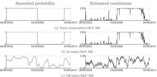
Figure 1: Overall commodity conditional correlations
Smoothed probability Estimated correlations
28/05/20030 15/09/2008 04/06/2014 1
28/05/20030.14 15/09/2008 04/06/2014 0.2
(a) Total commodities
28/05/20030 15/09/2008 04/06/2014 1 28/05/20030.17 15/09/2008 04/06/2014 0.24 (b) In-index commodities 28/05/20030 15/09/2008 04/06/2014 1 28/05/20030.03 15/09/2008 04/06/2014 0.14 (c) Off-index commodities
Note: this figure provides the estimated smoothed probability (left) and equally average correlation pairs of commodity futures daily returns (right), for the period between May 28, 2003 and June 4, 2014. Panel (a) contains results for the all commodity sample and the bottom two panels ((b) and (c)) reports results for respectively In- and Off-index commodity futures returns. The timeline of the figure in panels (a) and (b) indicates a correlation regime change on September 15, 2008, corresponding exactly to the Lehman Brothers demise. Regime One refers to the weaker correlation regime. Panel (c) indicates that correlations across Off-index commodity futures returns vary without regime change.
Figure 1 reports probabilities and the dynamics of the equally average correlation pairs of overall commodity futures returns. It is easy to see that the financial crisis period involves a new correlation regime between different commodity futures returns, with a regime change that coincides exactly with Lehman Brothers’ collapse on September 15, 2008. Furthermore, the transition matrix9 indicates that each regime is highly persistent with the probability of staying in a regime being higher than 0.99.10 The second regime, coinciding with the financial crisis and
the Lehman default, corresponds to an increase in magnitude of all correlations relative to those in the low correlation regime (Figure 1a). The equally weighted average of returns correlations of all commodity pairs increases from about 0.14 to 0.20, suggesting that commodity markets are
8
We use a different definition of In- and Off-index commodities from that of Tang and Xiong (2010, 2012). We consider commodities not only in the GSCI and the DJ-UBS but also in RICI and JF/RBC as "In-index", "Off-indexed" otherwise. We think that although the GSCI and DJ-UBS are the most important indices, the two others are not negligible in terms of trading volume (US dollar 55bn, 23bn, 1bn and 3.5bn, respectively). That being said, we do estimate correlations of Off-index commodities following the definition ofTang and Xiong(2010,
2012) and, as expected, we do not find a significant difference from those of In-index commodities. Results are not reported in the paper but available upon request.
9
Results are not reported but are available upon request.
10
It could be argued that, as inTang and Xiong(2010, 2012), the financialization process that began in 2004 may have led to a regime change in the dynamic correlation across commodities. Hence, as a robustness check, we estimated our model with three and even four regimes. Results clearly indicate the absence of an additional significant regime, and are available upon request.
driven more by broader trends than by fundamental factors specific to each market. This result confirms the "loss spiral" argument that correlations between unrelated assets increase in periods of extreme conditions. However, this argument suggests that dynamic correlations should have transitioned back to the low correlation regime as the financial crisis wound down in May 2009 and the recession in the US officially ended in June 2009. Our sample length covers a long enough period after the crisis to enable us to detect any return to the lower correlation regime (regime One). It is worth noting that regime One does seem to show up again on some occasions: very briefly in early 2010 and, in late 2012, and more frequently in 2013.
However, this result does not allow us to conclude firmly on the temporary nature of the financial crisis effect. Rather, it shows that the effect lasted longer than expected after the immediate crisis abated in 2009. It is true that the high financial asset volatility concomitant with the financial crisis, as measured by the VIX (see Figure 2 in the supplementary Appendix page 3), had ended by mid-2009, but two significant spikes emerge in May-October 2010 and August 2011-April 2012, which could have prolonged the initial effect of the 2007-2008 financial crisis. However, as the higher correlation regime extends beyond April 2012, the financial crisis cannot fully account for this regime. An alternative explanation might be that investors’ risk preferences were lastingly impacted by extreme events, outlasting the actual estimated shift in correlation.
On the other hand, Figure 1a shows that before the significant rise in the higher correlation regime (regime Two), dynamic correlations seem to initiate a slight increasing trend, confirming
Tang and Xiong(2010,2012)’s view and the “style”investment argument that the financialization process started impacting commodity correlations before the financial crisis. Moreover, as shown in Figure 1c, despite the absence of an identified regime change, Off-index commodity correla-tions are subject to a ceiling varying between 0.03 and 0.14, with more steady increases after the Lehman Brothers default. These results indicate a certain disconnection between Off-index commodities, providing additional evidence for the financialization effect in indexed commodi-ties, and confirm the findings ofBasak and Pavlova(2013) andTang and Xiong(2010,2012) that financialization affects not only In-index commodities but also, to a lesser extent, Off-index com-modities. However, our estimated average correlations of In- and Off-index commodities differ in magnitude from those of Tang and Xiong (2010, 2012). This difference may be due to different definitions of Off-index commodities and to different estimation methodologies.
However, the dynamic correlations of the overall sample may mask large variations among commodity groups. By analyzing specific groups, we identified three main types of switching dynamic (Figure11 in Appendix C). The special feature of the first group, composed of Grains, Softs, Livestock and Precious Metals (Figures11c,11d,11eand 11f, respectively), is that corre-lations vary, without identified regime switches, between 0.16 and 0.26, 0.05 and 0.18, 0.38 and 0.5, and 0.51 and 0.68, respectively. For the second group, composed of Energy commodities, we observe a different dynamic correlation path. The higher correlation regime (regime Two) starts well before the 2008 financial crisis, and regime One returns and firmly establishes it self at the end of fall 2012 (Figure11a); correlations then decline to even below their pre-crisis levels. This proves the temporary nature of the financial crisis effect on this group and would tend to reinforce the idea that the "loss spiral" mechanism triggered by the financial crisis was simply revealing the financialization and "style" investment process effect on the commodity returns correlation dynamics. By contrast, however, our findings on correlations across the third group, Industrial Metals, deserve particular attention: this group undergoes a regime change slightly after the Lehman Brothers demise on September 15, 2008 (Figure11b), and the weaker correlation regime (regime One) shows up again at the end of the sample. Moreover, it is worth noting the remark-able similarity between the dynamic correlations of this group and those of the overall sample, suggesting that the dynamic switching of the former drives that of the latter.
4.2 Co-movements between Non-Energy commodities and WTI
A complementary strategy to study dynamic correlations across commodities is to evaluate cor-relations of the constituent commodities with their index, as done in Barberis et al. (2005) for stock markets. Moreover, as by construction the index is correlated with its constituents, we use WTI as a proxy for commodity indices since it is the most heavily weighted commodity across the four commodity indices used in this study. This solution is also used by Tang and Xiong
(2010,2012). We first focus on correlations between the overall Non-Energy commodity sample and WTI; then we compare different commodity Non-Energy groups’ correlation with WTI; fi-nally, we separately treat the correlations of individual commodities with WTI to obtain greater detail. For these estimations, we construct three equally-weighted indices of Total, In-index and Off-index Non-Energy commodities. This allows us to estimate probabilities of regime change for dynamic correlations only between Non-Energy commodities and WTI, thereby eliminating those across Non-Energy commodities themselves.
Figure 2: Total Non-Energy commodity-WTI conditional correlations
Smoothed probability Estimated correlations
28/05/20030 14/07/2005 04/06/2014 1 Regime 1 28/05/20030 15/09/2008 28/09/2012 1 Regime 2 28/05/20030 14/07/2005 15/09/2008 28/09/2012 1 Regime 3 28/05/20030.21 15/09/2008 04/06/2014 0.71
(a) Total Non-Energy commodity-WTI
28/05/20030 14/07/2005 04/06/2014 1 Regime 1 28/05/20030 15/09/2008 28/09/2012 1 Regime 2 28/05/20030 14/07/2005 15/09/2008 28/09/2012 1 Regime 3 28/05/20030.21 15/09/2008 04/06/2014 0.71 (b) In-index Non-Energy/WTI 28/05/20030 15/09/2008 04/06/2014 1 28/05/20030.01 15/09/2008 04/06/2014 0.17 (c) Off-index Non-Energy/WTI
Note: this figure plots the estimated smoothed probability (left) and dynamic correlation of the equally-weighted indices of Non-Energy commodity futures returns with WTI (right), using daily data between May 28, 2003 and June 4, 2014. Panel (a) contains results from the equally-weighted index constructed from the total non-energy commodity futures returns. Panels (b) and (c) contain results from the equally-weighted indices constructed from In- and Off-index Non-Energy commodity futures returns, respectively. Results indicate three dynamic correlation regimes for Total and In-index commodities. While the weaker correlation regime (regime One) corresponds to the period preceding the financialization process, the higher correlation regime (regime Two) corresponds to the financial crisis period. Regime Three, the intermediate correlation regime, reflects commodity financialization. Only two regimes are identified for Off-index Non-Energy commodities: regime One and regime Two correspond respectively to the weaker and higher regimes.
Smoothed probabilities and the dynamic Non-Energy commodity index-WTI correlations in Figure2reveal several important results. First, the RSDC model detects three significant regimes corresponding to lower, intermediate and higher correlations. During the intermediate regime (regime Three), correlations followed a new upward trend, gradually going from about 0.20 in July 2005 to about 0.60 just before the Lehman Brothers collapse in September 2008. This may reflect the financialization effect and reinforces the "style" effect theory, confirming empirical findings byTang and Xiong(2010,2012) that the average correlation of Non-Energy commodity
Figure 3: Non-Energy commodity groups-WTI conditional correlations
Smoothed probability Estimated correlations
28/05/20030 14/07/2005 04/06/2014 1 Regime 1 28/05/20030 15/09/2008 28/09/2012 1 Regime 2 28/05/20030 14/07/2005 15/09/2008 28/09/2012 1 Regime 3 28/05/20030.08 15/09/2008 04/06/2014 0.62
(a) Industrial Metals/WTI
28/05/20030 14/07/2005 04/06/2014 1 Regime 1 28/05/20030 15/09/2008 28/09/2012 1 Regime 2 28/05/20030 14/07/2005 15/09/2008 28/09/2012 1 Regime 3 28/05/20030.18 15/09/2008 04/06/2014 0.67 (b) Agriculture/WTI 28/05/20030 14/07/2005 04/06/2014 1 Regime 1 28/05/20030 15/09/2008 28/09/2012 1 Regime 2 28/05/20030 14/07/2005 15/09/2008 28/09/2012 1 Regime 3 28/05/20030.14 15/09/2008 04/06/2014 0.64 (c) Grains/WTI 28/05/20030 14/07/2005 04/06/2014 1 Regime 1 28/05/20030 15/09/2008 28/09/2012 1 Regime 2 28/05/20030 14/07/2005 15/09/2008 28/09/2012 1 Regime 3 28/05/20030.13 15/09/2008 04/06/2014 0.54 (d) Softs/WTI 28/05/20030 15/09/2008 04/06/2014 1 28/05/20030.04 15/09/2008 04/06/2014 0.33 (e) Livestock/WTI 28/05/20030 15/09/2008 04/06/2014 1 28/05/20030.05 15/09/2008 04/06/2014 0.55 (f) Precious Metals/WTI
Note: this figure plots the estimated smoothed probability (left) and dynamic correlation of the equally-weighted indices returns, constructed from Non-Energy commodity futures groups (as defined in Section 3), with WTI (right), using daily data between May 28, 2003 and June 4, 2014. For instance, Panel (a) contain results from the equally-weighted index constructed from Industrial Metals futures returns. Results indicate three dynamic correlation regimes for Industrial Metals, Agriculture, Grains and Softs groups. The weaker correlation regime (regime One) corresponds to the period preceding the financialization process, the higher correlation regime (regime Two) corresponds to the financial crisis period. Regime Three, the intermediate correlation regime, reflects commodity financialization. Only two regimes, lower (regime One) and higher (regime Two) regimes, are identified for Livestock and Precious Metals.
futures returns with WTI started increasing well before the financial crisis. Second, correlation is indeed found to have increased significantly on September 15, 2008, to about 0.70, remaining high until September 2012. Importantly, therefore, our results for the first time reveal the temporary
nature of the financial crisis effect.
This is compelling evidence in support of the "loss spiral" argument and the market-of-one notion, implying a reversion to the lower pre-crisis correlation regime. As explained above, since the financial crisis officially ended in June 2009, the brief turbulent periods that followed between 2010 and mid-2012 may appear to have prolonged the financial crisis regime. A third important finding is that, correlations reverted to the pre-crisis level in a gradual manner: first the intermediate regime (regime Three) started to show up again in September 2012, before giving way to the lower correlation regime (regime One). Fourth, we find that Off-index Non-Energy commodity-WTI correlations rose to 0.17 during the financial crisis and reverted to pre-crisis levels in September 2012 (Figure 2c). Although correlations started to increase a little before the Lehman Brothers demise, our model did not separate out this relatively small upward trend as a fully-fledged regime.11 This finding further confirms the above-discussed theories and is
consistent with Tang and Xiong (2010, 2012) and Basak and Pavlova (2013), who found that financialization and, by implication, financial crisis effects are more pronounced on In-index than on Off-index commodity futures returns.
Other interesting findings are identified when analyzing the correlations of different Non-Energy commodity groups with WTI (Figure3).On the one hand, dynamic correlations between the different commodity groups (except for Precious Metals and Livestock) and WTI are char-acterized by three separate regimes. This is very similar to results from Total and In-index Non-Energy commodities. On the other hand, Livestock group-WTI correlations follow a differ-ent path: only two regimes are detected, with a low correlation regime until September 15, 2008, giving way to the high financial crisis regime, and appeared again at the end of September 2012. Precious Metals too highlights the heterogeneity in Non-Energy commodity-WTI correlations. Its dynamic correlations with WTI continually move between 0.05 and 0.55 without any identified regime change, reflecting its safe-haven status.
As for total Non-Energy commodities, indices for Non-Energy commodity groups are con-structed using equally-weighted commodity futures returns for each group. For robustness, we also apply an alternative measure using GSCI sub-index weights.12 Results are qualitatively similar and robust with the two alternative definitions of constructed indices (Figure 12). Fur-thermore, as a second robustness check, we estimate dynamic correlations between the available Non-Energy GSCI sub-indices, namely GSCI Industrial metals, Agriculture, Livestock and Pre-cious Metals, and WTI. Once again, our estimations give very similar results to those from constructed indices (Figure13 in Appendix C).
To further reveal commodity-specific characteristics, we decide to analyze each Non-Energy commodity-WTI correlation pair estimated using bivariate models, as a complement to the total and group analyses. The specific and independent switching dynamics of each pairwise correlation were examined. As expected, the timeline of the sub-figures in Figure 4 indicates a variety of commodity-WTI correlations in switching dynamics. More precisely, smoothed probabilities (Appendix C) show that for some bivariate estimations, three regime changes are detected (Figure
14), while only two regimes are identified for the others (Figure14). The common feature of Non-Energy individual commodity futures returns, except for barley, sunflowers and orange juice, is the steep jump in their correlations with WTI coinciding with either the financial crisis or the demise of Lehman Brothers. This confirms findings by Tang and Xiong (2010, 2012) that the correlation of Non-Energy commodities with WTI has increased, which is interpreted as evidence of the financialization of commodities. This is reinforced by the finding that individual Off-index commodities, such as barley and sunflowers, are totally disconnected with WTI, with correlations fluctuating around zero. Unlike previous studies, moreover, our results show the temporary nature of the recent hike in these correlations, which is due to the temporary large shock from
11
Transition matrix and smoothed probability clearly show the absence of a third regime. Results are available upon request.
12
Figu re 4: Biv ariate estimate d commo d it y-WTI corre lation s 28/05/2003 15/09/2008 04/06/2014 0.86 0.91 0.95 WTI/heating oil 28/05/2003 15/09/2008 04/06/2014 0.11 0.34 0.57 WTI/natural gas 28/05/2003 15/09/2008 04/06/2014 0.1 0.36 0.62 WTI/coal 28/05/2003 15/09/2008 04/06/2014 0.09 0.31 0.52 WTI/gold 28/05/2003 15/09/2008 04/06/2014 0.13 0.31 0.5 WTI/silver 28/05/2003 15/09/2008 04/06/2014 0.06 0.28 0.51 WTI/platinum 28/05/2003 15/09/2008 04/06/2014 0.06 0.3 0.54 WTI/palladium 28/05/2003 15/09/2008 04/06/2014 0.18 0.36 0.55 WTI/alluminium 28/05/2003 15/09/2008 04/06/2014 0.19 0.38 0.57 WTI/copper 28/05/2003 15/09/2008 04/06/2014 0.09 0.27 0.45 WTI/nickel 28/05/2003 15/09/2008 04/06/2014 0.02 0.28 0.54 WTI/lead 28/05/2003 15/09/2008 04/06/2014 0.06 0.27 0.47 WTI/tin 28/05/2003 15/09/2008 04/06/2014 0.14 0.33 0.52 WTI/zinc 28/05/2003 15/09/2008 04/06/2014 0.11 0.31 0.51 WTI/corn 28/05/2003 15/09/2008 04/06/2014 0.17 0.34 0.51 WTI/soybeans 28/05/2003 15/09/2008 04/06/2014 0.19 0.37 0.56 WTI/soybean oil 28/05/2003 15/09/2008 04/06/2014 0.05 0.31 0.58 WTI/wheat 28/05/2003 15/09/2008 04/06/2014 0.03 0.25 0.47 WTI/coffee 28/05/2003 15/09/2008 04/06/2014 0.09 0.24 0.39 WTI/cotton 28/05/2003 15/09/2008 04/06/2014 0.08 0.11 0.14 WTI/orange juice 28/05/2003 15/09/2008 04/06/2014 0.04 0.04 0.04 WTI/barley 28/05/2003 15/09/2008 04/06/2014 0.07 0.2 0.34 WTI/oats 28/05/2003 15/09/2008 04/06/2014 0.05 0.16 0.28 WTI/rice 28/05/2003 15/09/2008 04/06/2014 0.01 0.14 0.26 WTI/palm oil 28/05/2003 15/09/2008 04/06/2014 0.05 0.18 0.3 WTI/cocoa 28/05/2003 15/09/2008 04/06/2014 0.12 0.25 0.39 WTI/sugar 28/05/2003 15/09/2008 04/06/2014 −0.01 0.07 0.14 WTI/lumber 28/05/2003 15/09/2008 04/06/2014 −0.01 0 0 WTI/sunflowers 28/05/2003 15/09/2008 04/06/2014 0.04 0.12 0.21 WTI/lean hogs 28/05/2003 15/09/2008 04/06/2014 0.03 0.19 0.35 WTI/live cattle 28/05/2003 15/09/2008 04/06/2014 −0.02 0.14 0.3 WTI/feeder cattle 17
the financial crisis, as several agricultural, soft and oil individual futures return correlations return to their pre-crisis levels.
This is more consistent with the notion of a "market-of-one" and the "loss spiral" theory whith investors facing fire sales of liquid risky assets during periods of high volatility in financial markets. Interestingly, individual Industrial Metals commodities exhibit remarkable similarity, both with their group and with each other, in terms of timing of the change across regimes and the correlation spread value between low and high correlation regimes. The common turning point corresponds to the demise of Lehman Brothers, after which the higher correlations regime seems to be persistent, except for aluminum and zinc. On the other hand, correlations between individual Off-index commodity futures returns, except palm oil, with WTI are consistent with the expected theoretical findings and results from total Off-index commodities. Palm oil, however, behaves exactly like In-index commodity futures: its correlation with WTI sharply increases during the financial crisis period, reverting to its low level by the end of September 2012.
5
Co-movements between commodities and traditional assets
Several previous empirical studies examine the co-movement between commodity and equity re-turns with the objective of judging the diversification benefits of commodity futures as alternative assets in portfolios and assessing whether or not commodity and financial markets are becoming more closely integrated (Jensen et al. (2000),Erb and Harvey (2006), Chong and Miffre(2010),
Tang and Xiong(2010),Choi and Hammoudeh(2010),Büyükşahin et al.(2010),Silvennoinen and Thorp(2013), and Büyükşahin and Robe (2014)). In this section we first examine the dynamic correlation between commodities and the S&P 500, and second, we conduct the same analysis for commodity-bond co-movements.
5.1 Commodity-equity co-movements
The focus on commodity-equity co-movements is justified by the large weight of stocks in the commodity index investors’ portfolio. As explained in Tang and Xiong(2010), increasing invest-ment in commodity indices may have two opposing effects on co-moveinvest-ments between commodity indices and traditional asset returns such as stocks, depending on index investors’ rebalancing strategies and the composition of their portfolios. On the one hand, commodity index trading can act as a channel of higher correlations with equities in a portfolio, as index investors, hav-ing incentives to maintain their portfolio diversification level, rebalance their portfolios between commodities and stocks when shock alters portfolio weights (Basak and Pavlova(2013)). On the other hand, portfolio composition switches between commodities and stocks can generate a weak and even negative correlation between the two different asset classes. This effect ties in with the "style effect" theory (Barberis and Shleifer (2003)), which considers this negative correlation as a consequence of the style competition caused by the externality generated by switcher investors. To sum up, the overall commodity-equity co-movement reaction may depend on the combined effect of these two opposing forces, or on whether positive or negative effects prevail.
However, in times of financial crisis, regardless of the above effects, correlations may sharply increase between different asset classes comprising investors’ portfolios, particularly between com-modities and equities, the largest segment of investors’ portfolios (Kyle and Xiong (2001) and
Brunnermeier and Pedersen(2009)).
First, we present estimation results on commodity index-equity correlations using the four most popular commodity indices. Secondly, based on the above theories, we take a closer look at commodity-equity correlations through estimations using individual commodity futures returns.
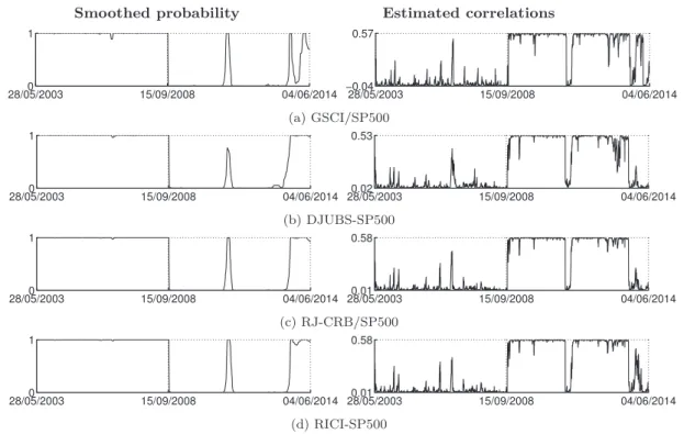
Figure 5: Commodity indices and the S&P 500
Smoothed probability Estimated correlations
28/05/20030 15/09/2008 04/06/2014 1 28/05/2003 15/09/2008 04/06/2014 −0.04 0.57 (a) GSCI/SP500 28/05/20030 15/09/2008 04/06/2014 1 28/05/20030.02 15/09/2008 04/06/2014 0.53 (b) DJUBS-SP500 28/05/20030 15/09/2008 04/06/2014 1 28/05/20030.01 15/09/2008 04/06/2014 0.58 (c) RJ-CRB/SP500 28/05/20030 15/09/2008 04/06/2014 1 28/05/20030.01 15/09/2008 04/06/2014 0.58 (d) RICI-SP500
Note: this figure plots the estimated smoothed probability (left) and dynamic correlation of commodity indices returns with S&P 500 (right), using daily data between May 28, 2003 and June 4, 2014. Results indicate two dynamic correlation switching regimes, regime One referring to the weaker correlation regime.
5.1.1 Commodity indices and the S&P 500
Figure 5 shows pairwise correlations among all four equity-commodity indices, namely GSCI, DJ-UBS, RJ-CRB and RICI.13Smoothed probabilities between the S&P500 and different indices follow a similar pattern, indicating a regime change precisely in September 15, 2008 following the Lehman bankruptcy. As indicated in the previous section, we estimate our model with no restriction on the number of regimes, and our estimations clearly support the existence of only two regimes. As we can see, during regime One, dynamic correlations between commodity indices and the S&P 500 are very low and even negative for the GSCI index, except for some insignificant fluctuations, before the dramatic upsurge to more than 0.5 in regime Two. This is in agreement with the findings ofGorton and Rouwenhorst(2006),Büyükşahin et al. (2010) and
Büyükşahin and Robe(2014), but contrary to those ofTang and Xiong(2010), who find that the correlation between the GSCI index and the S&P500 started to increase from 2004. As explained in Büyükşahin and Robe(2014), the rolling correlation technique can lead to biased estimation due to sensitivity to volatility. These results are therefore more consistent with the "style effect" theory, which documents the very weak correlation between competing asset classes or "styles", and their robustness to different commodity indices consequently runs counter to the theoretical findings of Basak and Pavlova (2013).
Evidence that the commodity-equity returns correlation was negligible prior to September 2008 and has increased sharply since then is not new, being frequently found in the literature (Gorton and Rouwenhorst (2006), Büyükşahin et al. (2010) and Büyükşahin and Robe(2014)). Our work clearly identifies a regime change in commodity-equity correlations, corresponding exactly to the Lehman Brothers collapse on September 15, 2008 when the prices of most tradable
13
We also estimate equity correlations with GSCI sub-indices. The focus on the GSCI index is justified by its very high market share (63%). Results from sub-indices (Figure16), especially GSCI Energy, are similar to those from the GSCI index, except for GSCI Precious metals, confirming the status of precious metals as a safe haven.