Simulation of ozone production in a complex circulation region using nested grids

HAL Id: hal-00328365

https://hal.archives-ouvertes.fr/hal-00328365

Submitted on 4 Jun 2004

HAL is a multi-disciplinary open access

archive for the deposit and dissemination of

sci-entific research documents, whether they are

pub-lished or not. The documents may come from

teaching and research institutions in France or

abroad, or from public or private research centers.

L’archive ouverte pluridisciplinaire HAL, est

destinée au dépôt et à la diffusion de documents

scientifiques de niveau recherche, publiés ou non,

émanant des établissements d’enseignement et de

recherche français ou étrangers, des laboratoires

publics ou privés.

region using nested grids

M. Taghavi, S. Cautenet, Gilles Foret

To cite this version:

M. Taghavi, S. Cautenet, Gilles Foret. Simulation of ozone production in a complex circulation region

using nested grids. Atmospheric Chemistry and Physics, European Geosciences Union, 2004, 4 (3),

pp.838. �hal-00328365�

SRef-ID: 1680-7324/acp/2004-4-825

Chemistry

and Physics

Simulation of ozone production in a complex circulation region

using nested grids

M. Taghavi, S. Cautenet, and G. Foret

Laboratoire de M´et´eorologie Physique, OPGC-CNRS and Universit´e Blaise Pascal, Aubi`ere, France Received: 2 February 2003 – Published in Atmos. Chem. Phys. Discuss.: 25 July 2003

Revised: 24 May 2004 – Accepted: 25 May 2004 – Published: 4 June 2004

Abstract. During the ESCOMPTE precampaign (summer 2000, over Southern France), a 3-day period of intensive ob-servation (IOP0), associated with ozone peaks, has been sim-ulated. The comprehensive RAMS model, version 4.3, cou-pled on-line with a chemical module including 29 species, is used to follow the chemistry of the polluted zone. This efficient but time consuming method can be used because the code is installed on a parallel computer, the SGI 3800. Two runs are performed: run 1 with a single grid and run 2 with two nested grids. The simulated fields of ozone, carbon monoxide, nitrogen oxides and sulfur dioxide are compared with aircraft and surface station measurements. The 2-grid run looks substantially better than the run with one grid be-cause the former takes the outer pollutants into account. This on-line method helps to satisfactorily retrieve the chemical species redistribution and to explain the impact of dynamics on this redistribution.

1 Introduction

During the last century, the atmospheric composition has been modified considerably by human activities. One of the consequences of this change is the high ozone concentrations observed in polluted zones. In recent years, high ozone con-centrations have been reported in the south of France, due to high anthropogenic and biogenic emissions. For this reason, southern France has chosen as the focus in the ESCOMPTE campaign (Cros et al., 2004). High concentrations of ozone and other photochemical oxidants have an impact on the lung function of human beings (Bates, 1995a, b) and are recog-nized as having negative effects on public health, crops and forests (Taylor, 1969; Heck et al., 1984). In order to study the transport of pollutants and their chemical regime, it is

Correspondence to: M. Taghavi

(m.taghavi@opgc.univ-bpclermont.fr)

hence very important to assess ozone production. For in-stance, the Current Directive 92/72/EEC for the European Union requires that the member states set and continually monitor the O3 thresholds, with emphasis on excess

con-centration cases (Gangoiti et al., 2002). A numerical model describing meteorology, pollutant emission, transport, chem-istry, and deposition is a powerful tool to address the problem of air quality and to develop effective control strategies. This type of model must undergo a validation step using reliable observational data, which ensures, to some extent, its accu-racy. In fact, some uncertainty is inevitable, because there are more than 3000 different chemical species in the atmo-sphere involved in complex chemistry. For instance, the ex-plicit oxidation mechanism of even one organic compound includes hundreds of reactions. Hence, the amount of reac-tions quickly becomes unmanageable for a VOC-NOx

mix-ture when the number of organics increases. An example of a complex explicit mechanism is the NCAR gas-phase mas-ter mechanism (Madronich and Calvert, 1989), with 4930 chemical reactions. Thus, there are three major problems: (i) a large CPU time is required for an explicit solution; (ii) the wide range covered by the chemical timescales leads to highly stiff systems which require specific solvers (Djouad and Sportisse, 2002); (iii), as a general rule, kinetic coeffi-cients and emission rates are not available for each organic species but for a whole group. As a result, these explicit chemical mechanisms are not used in pollution studies ex-cept to describe the inorganic NOx chemistry, which is

rel-atively straightforward. Condensed schemes are therefore commonly used (Aumont et al., 1996).

The chemistry/transport models can be coupled either on-line or offon-line with meteorological models. In the “offon-line” case, the frequency of the sampling rate of the meteorologi-cal fields must be considered with regards to transport. For example, a 3-h frequency is used in the offline coupling of the LOTOS model (VanLoon et al., 2000) whereas a 1-h fre-quency is taken for TVM (meteorological model) coupled

offline with the chemistry model RACM (Thunis and Cuve-lier, 2000). It is obvious that in these cases we cannot have good accuracy in the species transport, because the meteo-rological data are averaged in time. The emission rates and the transport play an important role in the chemistry regime for the mesoscale studies, especially in the case of complex circulation. For instance, if we use a 3-hourly meteorolog-ical dataset, a problem arises during the afternoon, as at 16:00 LST, we may be in a sea breeze regime; whereas at 19:00 LST, the land breeze onset already may be effective. On the other hand, the offline method is useful in large scale studies.

The lateral boundary conditions may represent another se-rious problem. As a general rule, in offline mode, model-ers derive boundary conditions either from measurements or from clean air values. These values are held constant and homogeneous along large parts of the boundary. However, Winner et al. (1995) showed that the boundary values can strongly impact the simulation quality. In other words, one must pay close attention to the boundary conditions. To get rid of this problem, we use a nested grid approach. This is a quite common practice in meteorological mesoscale model-ing, but it is a new method in chemistry/transport modeling. With the nested grid method, the pollutant concentration ar-riving at the boundary of a fine grid depends on time and on the location of the boundary grid point. This method takes into account the pollutant sources far from the studied do-main (the finest grid).

The aim of this study is to develop a chemistry/transport model which reconciles two antagonistic requirements: a minimum CPU time and a maximum accuracy. To this end, we use an online coupling between the meteorological and the photochemical models with two nested grids, since com-puters like SGI 3800 are very powerful and fast for paral-lel codes. We have coupled online the RAMS (Regional Atmospheric Modeling Systems) mesoscale model (Cotton et al., 2003) with the MOCA 2.2 chemical model (Aumont et al., 1996). This coupled model is hereafter referred to as “RAMS-chemistry”. We have focused on transport, dy-namics impact, and chemical redistribution from primary or secondary species.

In this paper, we summarize the context of the ES-COMPTE precampaign. Then we present the emission database and the meteorological model. We examine the me-teorological conditions during the pollution period and com-pare the modeled meteorological fields with the observed values (surface station and aircraft measurements). Then, we describe the chemistry mechanism (code MOCA 2.20) cou-pled online with RAMS. In the fine grid, we compare the modeled ozone, carbon monoxide, nitrogen oxides, and sul-fur dioxide fields with aircraft and surface observations. Fi-nally, we discuss the role of dynamics in the redistribution of the modelled species.

2 ESCOMPTE pre-campaign

The ESCOMPTE precampaign was conducted in June and July 2000 in southeastern France (http://medias.obs-mip.fr/ escompte). During this period, an Intensive Observation Pe-riod (IOP0) took place on 29, 30 June and 1 July. For these three days, data from meteorological and chemical surface stations and aircraft measurements are available. For the modeling group, the aim of this precampaign was to perform runs in order to derive flight plans and to find the best loca-tions for the surface staloca-tions. Moreover, it was projected that the chemical and meteorological data gathered during this period would be useful to validate the models.

The detailed IOP0 database consists of: (i) the anthro-pogenic and biogenic emission inventory, with two different resolutions (15 km and 3 km); (ii) information about mete-orological conditions during the pollution period; (iii) sur-face measurements (fixed and mobile stations) for both me-teorological and chemical data; (iv) airborne measurements (aircrafts and balloons). Two aircrafts were operated: the PIPER AZTEC plane (M´et´eoFrance) and the INSU (Institut National des Sciences de l’Univers) ARAT plane. Several flights occurred during the studied days. Some of the main objectives of the ESCOMPTE campaign were to answer the following questions:

1. What is the respective role of the various dynamic and chemical mechanisms on the pollutant redistribution? 2. How should urban emissions be taken into account in

regional or global models?

3. Can we develop an operational forecast of pollution pe-riods?

4. What strategy should be developed in order to reduce the pollutant concentrations?

3 Meteorological modelling description

The RAMS model (Regional Atmospheric modelling Sys-tem; http://www.atmet.com; Cotton et al., 2003) is a parallel mesoscale model allowing the simulation of meteorological fields with horizontal scales spanning from one kilometer to a thousand kilometers. It includes nested grids. Many inves-tigations on regional pollution were previously made using the RAMS model (Lyons et al., 1995; Millan et al., 1997; Edy and Cautenet, 1998; Cautenet et al., 1999; Poulet et al., submitted, 20041).

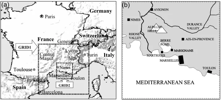
Simulations have been performed using two nested grids simultaneously to take synoptic and local circulations into account. In a simulation with two nested grids, each grid cov-ering a particular domain size (Fig. 1), a two-way interactive

1_{Poulet, D., Cautenet, S., and Aumont, B.: Simulation of the}

chemical impact of the bush fires emissions, in central africa, during the EXPRESSO campaign, submitted to J. Geophys. Res., 2004.

MARSEILLES MARTIGUES BERRE POND

MEDITERRANEAN SEA

MEDITERRANEAN SEA

(b)

(a)

pyrenees

Paris

Barcelona

Spain

Turin

Marseille Toulon

Toulouse

Switzerland

Geneva

Germany

Central

Massif

Alps

France

France

Italy

Lyons

France

France

Marseilles

Toulouse

Fig. 1. (a) Geographical map and configuration of nested grids, grid 2 represents the ESCOMPTE domain; (b) a zoom on grid 2 with location

of some observation stations.

process is involved. Grid 1 covers southern France, a part of Northern Spain and a part of Northern Italy, resulting in 36 square meshes of 15 km. Grid 2 represents the ESCOMPTE domain. It has 52 meshes of 3 km. We use a time step of 10 s and 35 levels in the vertical dimension (the same in both grids) with 15 levels from surface to 1500 m, which ensures a fine description of the boundary layer. The coarse domain in-cludes the cities of Lyons, Turin, and Barcelona, to the north, east and southwest respectively. Moreover, it comprises the Pyren´ees, Massif Central and Alps mountain ranges. This topography introduces a complex circulation associated with sea breeze. In the fine grid (grid 2), we have the cities of Marseilles, Toulon and Avignon, with the Alpilles hills and the Durance and Rhone valleys.

In the model, the initial meteorological fields and the 6-h-nudging are provided by the ECMWF (European Centre for Medium-Range Weather Forecasts) database. The sim-ulation starts on 28 June 2000 at 00:00 UTC and ends on 1 July 2000 at 21:00 UTC. The soil vegetation model includes 30 classes issued from USGS (United States Geophysical Survey) with a 1 km resolution. The “patches” configura-tion (Cotton et al., 2003) allows part of the 1 km informaconfigura-tion to be retained. The USGS topography also has a 1 km res-olution and an interpolation is performed. The sea surface temperature is obtained from Meteosat. Near the coastline, these temperatures are corrected using the OOM (Observa-toire d’Oc´eanographie de Marseille) shore temperature.

In this run, the reflected envelope topography scheme is used and aims to preserve both barrier heights and val-ley depths. The vertical diffusion is computed from the Smagorinsky scheme (Tripoli and Cotton, 1982), where

ad-justments to the vertical exchange coefficients are made us-ing a Richardson number/moist Brunt-Vaisala frequency en-hancement factor. The full microphysics scheme is not im-plemented, because it is an event of fair weather, but the con-densed water is calculated and the cloud cover is taken into account in the radiation code (Chen and Cotton, 1988).

4 Emissions

4.1 Anthropogenic emissions

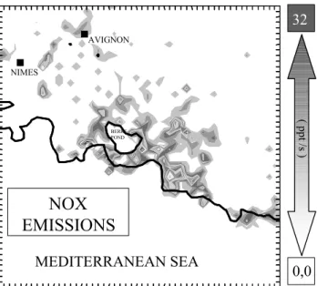
A key point of atmospheric chemistry is the influence of hu-man activity on emissions. For example, huhu-mans have dou-bled the natural rate of nitrogen fixation (Vitousek et al., 1997). In fact, one of the important reasons to study atmo-spheric chemistry in southeastern France is the high level of anthropogenic emissions due to the presence of many indus-trial factories, oil refineries, EDF (France Electricity) power stations and other large factories such as “Air Liquid”, situ-ated in the industrial zones of Fos-Sur-Mer or Berre Pond. Additional emissions are due to highways and polluted cities like Marseilles and Toulon on the coast, Aix-en-Provence or Avignon inland. These high anthropogenic emissions are il-lustrated in Fig. 2 where the NOx emissions are shown at

12:00 UTC for a typical July working day. 4.2 Biogenic emission

This region is covered by Mediterranean vegetation and pro-vides important biogenic emissions. This type of vegetation exhibits an annual cycle of biogenic emissions characterized by a rapid growth in March, a maximum in July-August and

NOX

EMISSIONS

MEDITERRANEAN SEA

32

0,0

Fig. 2. NOxemission map for an ordinary day of July at 12:00 UTC.

a strong decrease in September-October. Isoprene appears as the most abundant species (Simon et al., 2001). This com-pound is due mainly to Holm oak. In Fig. 3, we can see the isoprene emissions at 12:00 UTC for an ordinary day of July. 4.3 Database

For grid 1 with a resolution of 15 km, the emissions were obtained from the GENEMIS database. For the fine do-main (grid 2), we used an inventory derived from GENE-MIS, which we have added area sources for the industrial and urban regions from data of 1994 (http://medias.obs-mip. fr/escompte/projet/index.fr.php). For both grids, emissions were calculated from data of 1994 for anthropogenic emis-sions and 1997 for biogenic emisemis-sions. Hourly values were supplied for each mesh and for two days: (5 and 6 July 1994) for anthropogenic sources and (21 and 22 July 1997) for bio-genic sources. An inventory with a high resolution and up-dated emissions, specially performed for the ESCOMPTE domain must be available in 2004 (Franc¸ois et al., 2004; Taghavi et al., 2004).

5 The two ways nesting method

In mesoscale chemical and meteorological modeling, the boundary conditions must be specified. Modeling can be strongly influenced by them, especially when there is a strong flow crossing the borders. For chemistry/transport models, the existence of a high emission zone near the stud-ied domain can be significant because a strong wind may transport a large amount of the emitted pollutants from the outside source into the model domain. The boundary con-ditions can be provided by global modeling results which

MARSEILLES MARTIGUES BERRE POND

MEDITERRANEAN SEA

ISOPRENE

EMISSION

1,8

0,0

Fig. 3. Isoprene emission map for an ordinary day of July at 12:00 UTC.

generally have a resolution of about 100×100 Km or more. This crude resolution is not sufficient to obtain realistic re-sults with respect to chemistry. In our study, we wanted to realistically retrieve the chemical fields in grid 2. In fact, the coarse grid or grid 1 (15×15 Km) was used to provide boundary values for the fine grid or grid 2 (3×3 Km). The two way nesting method is very effective to obtain realistic simulations because at each time step, the fine grid (grid 2) provides its data to the coarser (mother) grid, which in turn forces the fine (daughter) grid. The two grids communicate with each other in a two-way scheme described by Clark and Farley (1984) and Walko et al. (1995). In particular, such a scheme allows emissions far outside grid 2 to influence the pollutant budget within grid 2. This method helps to explain the impact of pollutants emitted from Lyons, Barcelona, and Turin that are transported to the ESCOMPTE region. The pollutants from Lyons are channeled along the Rhone val-ley and have an impact on the ozone production in the ES-COMPTE domain.

6 High-resolution meteorological simulation: compari-son with surface station and airborne measurements The redistribution of pollutants and therefore the ozone pro-duction is very dependent on the meteorological conditions. The observed meteorological situation during IOP0 ranged between clear to slightly cloudy conditions. These con-ditions promote significant photochemical activity. On 29 June, wind direction was west to northwest (Mistral), and wind speed was from moderate to strong, locally exceed-ing 12 ms−1. The maximum temperatures reached about 29– 30◦C. On 30 June, the wind turned from north to west, and a

AVIGNON 0 5 10 15 20 25 30 35 0 4 8 12 16 20 24 28 32 36 40 44 48 52 56 60 64 68 Time (hour) Te mper autre (° C) Observed Modelled MARSEILLES 0 5 10 15 20 25 30 35 0 4 8 12 16 20 24 28 32 36 40 44 48 52 56 60 64 68 Time (hour) Temperature (° C) Observed Modelled TOULON 0 5 10 15 20 25 30 35 0 4 8 12 16 20 24 28 32 36 40 44 48 52 56 60 64 68 Time (hour) T e m p era tu re (°C ) Observed Modelled AVIGNON 0 1 2 3 4 5 6 7 8 9 0 4 8 12 16 20 24 28 32 36 40 44 48 52 56 60 64 68 Time (hour) Win d Sp eed ( m /s) Observed Modelled MARIGNANE 0 2 4 6 8 10 12 14 0 4 8 12 16 20 24 28 32 36 40 44 48 52 56 60 64 68 Wind Speed (m/s) Observed Modelled TOULON 0 2 4 6 8 10 12 0 4 8 12 16 20 24 28 32 36 40 44 48 52 56 60 64 68 Time (hour) Win d Sp ee d ( m /s) Observed Modelled MARSEILLES 0 1 2 3 4 5 6 7 8 9 0 4 8 12 16 20 24 28 32 36 40 44 48 52 56 60 64 68 Time (hour) Wind Speed (m/s) Observed Modelled MARIGNANE 0 5 10 15 20 25 30 35 0 4 8 12 16 20 24 28 32 36 40 44 48 52 56 60 64 68 Time (hour) T e m p ratu re (° C) Observed Modelled Time (hour)

Fig. 4. Time variation (UTC) of temperature and wind speed from 29 June–1 July 2000 for 4 cities, Avignon inland in north of ESCOMPTE

domain, Marignane in center, Marseilles and Toulon on the coast.

sea breeze developed in the afternoon with speeds from 4 to 7 ms−1. The maximum temperatures were around 30◦C. On 1 July, the sea breeze was enhanced by a southwest flow and the speeds were slightly greater: 5 to 8 ms−1, and the maxi-mum temperatures were lower than the day before (between 25◦C and 30◦C). On 30 June, the conditions which promote the formation of ozone peaks were fulfilled, i.e. high temper-ature and weak wind.

To validate the simulated meteorological fields, we com-pared the model results with surface station and airborne measurements. Some of these comparisons are shown in Figs. 4 and 5. To compare the model results with the sta-tion data, we use a statistical method (Cai and Steyn, 2000).

In fact, we have many stations (about 5) for each of the 4 towns in the model area (Marseilles, Marignane, Toulon and Avignon). These data can be strongly influenced by local effects. Marseilles and Toulon are located near the coast, Marignane lies in the center of the domain and Avignon is the furthest inland. The hourly station data comes from av-eraged data taken at 15-min intervals. In Fig. 4, we note that the observed and the modeled temperature values for the three days are in good agreement for all the surface stations. It is the same for the wind speed (Fig. 4). However, we re-mark that in Marignane, located close to pollutant sources (Figs. 1b and 2), the wind speed reaches the highest values (12 ms−1_{) on 29 June. This favors pollutant dispersion. We}

0 2 4 6 8 10 12 14 16 18 W ind Spe ed (m /s) Observed Modelled 13:15 13:30 13:45 14:00 14:15 14:30 14:45 15:00 15:15 15:30 15:45 UTC (Hour) 0 30 60 90 120 150 180 210 240 270 300 330 360 Wi nd D irect ion (d egree) Observed Modelled 13:15 13:30 13:45 14:00 14:15 14:30 14:45 15:00 15:15 15:30 15:45 UTC (Hour) 13:15 13:30 13:45 14:00 14:15 14:30 14:45 15:00 15:15 15:30 15:45 UTC (Hour) 0 5 10 15 20 25 30 35 P o ten ti al Tem p erature (° C) Observed Modelled 13:15 13:30 13:45 14:00 14:15 14:30 14:45 15:00 15:15 15:30 15:45 UTC (Hour) 0 10 20 30 40 50 60 70 Spe c if ic H u midity ( gr /k g) Observed Modelled 13:15 13:30 13:45 14:00 14:15 14:30 14:45 15:00 15:15 15:30 15:45 UTC (Hour)

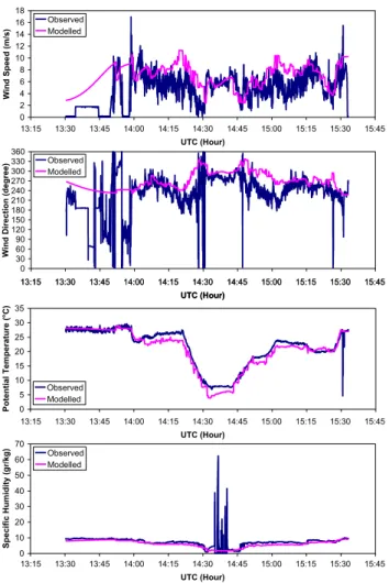
Fig. 5. Wind speed and direction, potential temperature and

spe-cific humidity for the AZTEC plane (flight of 30 June 2000 at 13:59 UTC).

note also that on the next two days, winds are weaker, with maximum values around 8 ms−1at midday.

With respect to airborne data, (Figs. 5 and 6), tempera-ture, specific humidity, wind speed, and direction measure-ments are in good agreement with model values. However, we note some essentially small differences for specific hu-midity, wind speed and direction around 14:38 UTC and 15:07 UTC (Fig. 5). At these times, the AZTEC plane flew at low levels (Fig. 7, where the altitude is drawn versus time). For the ARAT plane, we note that the measured wind speed and direction are slightly different from model values around 10:40 UTC (Fig. 6) in the free troposphere (Fig. 7), and around 12:30 UTC (Fig. 6) in the lower levels (Fig. 7). Fi-nally, we can say that the simulated meteorological fields are very realistic and that they do not induce a bias for the chem-ical fields. 0 5 10 15 20 25 Wi nd S p eed (m/ s) Observed Modelled 0 10:00 10:15 10:30 10:45 11:00 11:15 11:30 11:45 12:00 12:15 12:30 12:45 13:00 13:15 UTC (Hour) 0 30 60 90 120 150 180 210 240 270 300 330 360 Wind Dire ct io n (de g re e) Observed Modelled 0 10:00 10:15 10:30 10:45 11:00 11:15 11:30 11:45 12:00 12:15 12:30 12:45 13:00 13:15 UTC (Hour) 0 5 10 15 20 25 30 35 40 45 P o tenti a l Tem perature (°C ) Modeled Observed 0 10:00 10:15 10:30 10:45 11:00 11:15 11:30 11:45 12:00 12:15 12:30 12:45 13:00 13:15 UTC (Hour) 0 2 4 6 8 10 12 14 16 18 Spe c if ic H u midit y ( g r/k g) Observed Modelled 0 10:00 10:15 10:30 10:45 11:00 11:15 11:30 11:45 12:00 12:15 12:30 12:45 13:00 13:15 UTC (Hour)

Fig. 6. Wind speed and direction, potential temperature and specific

humidity for ARAT plane (flight of 1 July 2000 at 10:03 UTC).

7 Chemical model

The mechanism of the chemical model is given in Ap-pendix 1. It is a condensed version of the MOCA 2.20 model (Aumont et al., 1996). It takes 29 species and 64 re-actions into account. It describes the main processes driv-ing the changes in ozone concentration in a polluted zone. The hydroperoxyl/aldehyde conversion allows a description of the degradation of the various organic compounds from anthropogenic emissions. It involves the 3 main pathways of isoprene oxidation (a species strongly emitted by Mediter-ranean forests). Our chemical module calculates PAN con-centration, which allows a representation of the NOx

trans-port. Finally, the chemical module includes the NO3/N2O5

equilibrium for night chemistry. It has been validated by the intercomparison protocol proposed by Kuhn et al. (1998) and Poppe et al. (1996).

The chemical solver is the QSSA or Quasi Steady State Approximation (Hesstvedt et al., 1978), faster than a matrix solver such as the Gear solver (Gear, 1971) but quite accu-rate (Shieh et al., 1988; Dabdud and Seinfeld, 1995; Saylor

AZTEC Aircraft (2000, June 30) 0 10 20 30 40 50 60 70 80 90 100 O zone ( ppb) 0 500 1000 1500 2000 2500 3000 3500 Altit ude (m ) Observed Modelled (Run1) Modelled (Run2) Altitude 13:45 14:00 14:15 14:30 14:45 15:00 15:15 15:30 15:45 UTC (Hour)

ARAT Aircraft (2000, July 1)

0 10 20 30 40 50 60 70 80 90 100 Oz on e (pp b) 0 200 400 600 800 1000 1200 1400 1600 1800 Al titud e (m ) Observed Modelled (Run1) Modelled (Run2) Altitude 10:00 10:15 10:30 10:45 11:00 11:15 11:30 11:45 12:00 12:15 12:30 12:45 13:00 13:15 UTC (Hour)

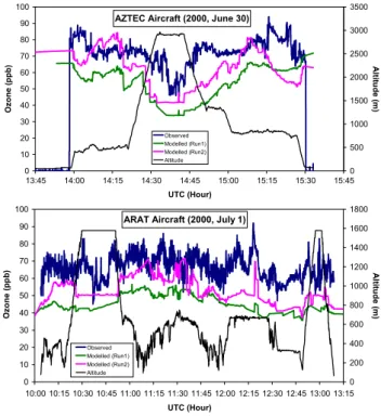
Fig. 7. Ozone concentration, observed with AZTEC plane (30 June

2000) and ARAT plane (1 July 2000), and modelled using only one grid (run 1) and using two nested grids (run 2).

and Ford, 1995). At each time step and each mesh, chem-ical rates are evaluated from temperature and pressure as calculated in the RAMS model. Photolysis rates are esti-mated from the Madronich model (Madronich, 1987), which takes the solar incident radiation and the molecular proper-ties of the atmospheric gases into account. The photolysis rates are updated every five minutes. Actinic fluxes are esti-mated by Eddington approximation (Joseph et al., 1976; Wis-combe, 1997). Three photolysis reactions, not integrated in Madronich’s program, have been added to this model. Quan-tum yield and absorption efficiency are derived from Aumont et al. (1996).

To reduce the CPU time, we have developed an original way of chemical constant rates evaluation (Poulet et al., sub-mitted, 2004)2. Chemical kinetic coefficients are calculated from a complex expression dependent on temperature and pressure. Since temperature and pressure vary on each mesh, calculations are made for each of them and thus require a very long time. In our code, a lookup table has been created for each chemical kinetic coefficient before simulation for all the typical temperature and pressure conditions in the atmo-sphere. So, during the run, RAMS-chemistry merely chooses the coefficient fitted to the current meteorological conditions in the lookup table. The interest of such a method with

par-2_{Poulet, D., Cautenet, S., and Aumont, B.: Simulation of the}

chemical impact of the bush fires emissions, in central africa, during the EXPRESSO campaign, submitted to J. Geophys. Res., 2004.

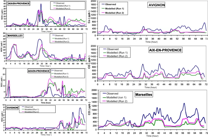
MARIGNANE 0 10 20 30 40 50 60 70 80 0 4 8 12 16 20 24 28 32 36 40 44 48 52 56 60 64 68 72 Time (hour) O zone ( ppb) Observed Modelled (Run1) Modelled (Run2) AVIGNON 0 10 20 30 40 50 60 70 80 0 4 8 12 16 20 24 28 32 36 40 44 48 52 56 60 64 68 72 Time (hour) O zon e (p pb ) Observed Modelled (Run1) Modelled (Run2) 0 10 20 30 40 50 60 70 Ozone (ppb) Observed Modelled (Run1) Modelled (Run2) MARSEILLES 0 4 8 12 16 20 24 28 32 36 40 44 48 52 56 60 64 68 72 Time (hour) TOULON 0 10 20 30 40 50 60 70 80 90 Ozone (ppb) Observed Modelled (Run1) Modelled (Run2) 0 4 8 12 16 20 24 28 32 36 40 44 48 52 56 60 64 68 72 Time (hour)

Fig. 8. Time variation (UTC) of observed and modelled (run 1 and

run 2) ozone concentration (ppb) from 29 June–1 July 2000 for 4 cities: Avignon inland in north of ESCOMPTE domain, Marignane in center, Marseilles and Toulon on the coast.

allel code is that CPU time is short: it allows a significant reduction in the simulation time (for SGI 3800 computer: 1 h 30 CPU for a simulated day).

8 Chemical results

In the ESCOMPTE region, the emissions are mainly of anthropogenic origin along coast (Fig. 2), and especially around the Berre Pond, but there are also biogenic emissions from the forest inland (Fig. 3). In the troposphere, ozone production is dependent on many different parameters, such as dynamical condition, radiation intensity, NOx/VOC ratio,

etc. It is sensitive to VOC and NOxemissions (Weimin et al.,

1997). The maximum in ozone occurs when there is a high concentration in VOC and NOx due to emission or

trans-port (Dodge, 1997b; Finlayson-Pitts and Pitts Jr., 1993). The sensitivity of ozone production to each of these parameters is variable. If one of these parameters is not correctly ac-counted for, an error in ozone estimation occurs.

AVIGNON 0 200 400 600 800 1000 1200 1400 1600 1800 2000 Co ( ppb ) Observed Modelled (Run 1) Modelled (Run 2) AIX-EN-PROVENCE 400 600 800 1000 1200 1400 1600 1800 2000 2 3 Time (hour) CO ( ppb

) Modelled (Run 1)Modelled (Run 2)

Marseilles 0 200 400 600 800 1000 1200 Time (hour) CO ( ppb Modelled (run 1) Modelled (Run 2) 0 200 400 600 800 1000 1200 1400 1600 1800 2000 AIX-EN-PROVENCE 400 600 800 1000 1200 1400 1600 1800 2000 2 3 Observed Modelled (Run 1) Modelled (Run 2) Marseilles 0 200 400 600 800 1000 1200 Observed Modelled (run 1) Modelled (Run 2) AIX-EN-PROVENCE 0 5 10 15 20 25 30 35 40 45 50 0 4 8 12 16 20 24 28 32 36 40 44 48 52 56 60 64 68 72 Time ( hour ) N O X ( ppb ) Observed Modelled (Run 1) Modelled (Run 2) MARSEILLE 0 5 10 15 20 25 30 35 40 45 50 0 4 8 12 16 20 24 28 32 36 40 44 48 52 56 60 64 68 72 N O X ( ppb ) Observed Modelled (Run 1) Modelled (Run 2) AVIGNON 0 1 2 3 4 5 6 7 8 9 10 0 4 8 12 16 20 24 28 32 36 40 44 48 52 56 60 64 68 72 Time ( hour ) SO 2 ( ppb ) Observed Modelled (Run 1) Modelled (Run 2) AIX-EN-PROVENCE 0 5 10 15 20 25 0 4 8 12 16 20 24 28 32 36 40 44 48 52 56 60 64 68 72 Time (hour) SO 2 ( ppb ) Observed Modelled (Run 1) Modelled (Run 2) AIX-EN-PROVENCE 0 5 10 15 20 25 30 35 40 45 50 0 4 8 12 16 20 24 28 32 36 40 44 48 52 56 60 64 68 72 Observed Modelled (Run 1) Modelled (Run 2) MARSEILLES 0 5 10 15 20 25 30 35 40 45 50 0 4 8 12 16 20 24 28 32 36 40 44 48 52 56 60 64 68 72 Time ( hour ) Observed Modelled (Run 1) Modelled (Run 2) AVIGNON 0 1 2 3 4 5 6 7 8 9 10 0 4 8 12 16 20 24 28 32 36 40 44 48 52 56 60 64 68 72 Observed Modelled (Run 1) Modelled (Run 2) AIX-EN-PROVENCE 0 5 10 15 20 25 0 4 8 12 16 20 24 28 32 36 40 44 48 52 56 60 64 68 72 Time (hour) Observed Modelled (Run 1) Modelled (Run 2) 0 4 8 12 16 20 24 28 32 36 40 44 48 52 56 60 64 68 72 Time (hour) 0 4 8 12 16 20 24 28 32 36 40 44 48 52 56 60 64 68 200 200 0 0 0 4 8 12 16 20 24 28 3 0 4 8 12 16 20 24 28 3 66 4040 4444 4848 5252 5656 6060 6464 6868 7272 2000 1800 1600 1400 ) 0 4 8 12 16 20 24 28 32 36 40 44 48 52 56 60 64 68 72 1400 1600 1800 2000 0 4 8 12 16 20 24 28 32 36 40 44 48 52 56 60 64 68 72

Fig. 9. Time variation (UTC) of observed and modelled (run 1 and run 2) NOx, SO2and CO concentration (ppb) from 29 June–1 July 2000

for 3 cities: Avignon inland in north of ESCOMPTE domain, Aix-en-Provence close to center and Marseilles in shore.

The quality of the chemical fields depends in particular on the meteorological fields themselves. As they are quite real-istic (see Sect. 6), we can study the impact of dynamics on the redistribution of chemical species. We will examine the role of nested grids to retrieve these mechanisms. However, we must keep in mind that, in this work, the emission in-ventory originates from a 1994 database, which may not be completely adequate.

Two runs are performed: run 1 with one grid, grid 2, which represents the ESCOMPTE region and run 2 with two nested grids (grid 1 including grid 2). To evaluate the ability of the RAMS-chemistry model, we compare the aircraft and sur-face station measurements with our numerical results. Dur-ing the run, at each time step, the coordinates of aircraft (al-titude, la(al-titude, longitude) are noted and the fitted numerical values are written in a file. Thus the modeled values cor-respond exactly to the same place and the same time as the aircraft measurements.

8.1 Aircraft measurements

Figure 7 presents the comparisons between model results and airborne data during IOP0 for run 1 and run 2. For both flights (AZTEC and ARAT planes), the modeled ozone curve

follows the observed ozone curve (same maximum and mini-mum), with, however, a weak but systematic underestimation in the modeled values. We think this difference could orig-inate for two reasons: (i) our chemical model includes the main species but not all, and (ii) errors can exist in emis-sions rates data and in source locations. Recall that the emissions were calculated from a 1994 database for anthro-pogenic emissions and from a 1997 file for biogenic emis-sions. When the aircraft altitude is high, i.e. when the mea-surements are performed within the free troposphere, we note weak ozone values. For the lower levels, near the surface, the values are generally high, except for the landing or take off periods. Planes took off and landed at Marignane airport, which is very close to high emissions sources of NOx and

they flew at low altitudes over smokestacks. Therefore, as there is a high NOxconcentration, the ozone titration is very

probable, especially in the absence of a sufficient amount of VOC. In other words, the NOx/VOC ratio is not favorable for

ozone formation (Finlayson-Pitts and Pitts Jr., 2000). How-ever, we remark that for both flights run 2 gives better results than run 1, because it takes the pollution from grid 1 into account.

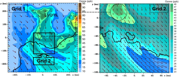
Grid 2

Grid 1

Grid 2

Lyons

Fig. 10. Ozone concentration (ppb) and Wind speed (ms−1) – Left: grid 1; right: grid 2; 29 June 2000 at 09:00 UTC.

8.2 Surface stations

For a sample of 4 selected surface stations, the numerical results are compared with the ozone, carbon monoxide, ni-trogen oxides, and sulphur dioxide observations. Figure 8 shows that for these stations, the ozone results of run 2 fit the observations better than run 1. In Avignon, a town lo-cated to the north of grid 2 (Fig. 1), on 29 and 30 June (01:00 UTC to 48:00 UTC), the ozone values are higher than on 1 July (48:00 UTC to 72:00 UTC). On 29 June, the val-ues are greater than 70 ppb because of transport of pollu-tants from northern areas. On the contrary, in Marignane, Toulon and Marseilles, towns located near the coast (Fig. 1), the ozone maxima are found for 30 June. During this day, the wind is weak and the sea breeze is well developed. We have a maximum of 80 ppb at Toulon and 70 ppb at Marig-nane. Figure 9, for two stations (Marseilles and Aix), the NOxmeasurements are slightly different from numerical

re-sults for both runs. Again, we note that run 2 is always better than run 1. The observations show that the NOxare limited

only for Aix on 29 June. The same occurs at Aix and Mar-seilles on 1 July (which is Saturday). The NOxlevels are very

strong for both towns on 30 June which is Friday (a day of departure for summer holidays). Figure 9, we can see the CO variations for the three days. The levels are high, particularly on 30 June and 1 July. The numerical results are better for the first day (where the traffic is regular) than the following days. In Fig. 9, we display the time evolution of the SO2

con-centration for two stations (Aix and Avignon). In Aix, there is local SO2emission. On the first day (29 June), we have

a Mistral wind (northwesterly), and in this case, the morn-ing SO2peak is quickly dispersed. On the following days,

we have a sea-breeze circulation (30 June) associated with

27 27,5 28 28,5 29 29,5 30 30,5 31 31,5 32 32,5 33 33,5 34 34,5 35 35,5 36 27 27,5 28 28,5 29 29,5 30 30,5 31 31,5 32 32,5 33 33,5 34 34,5 35 35,5 36 Ozone (ppb)

Fig. 11. Horizontal cross section for ozone concentration (ppb), 29

June 2000 at 09:00 UTC, grid 2 – simulation with one grid (run 1).

synoptic Southerly flow (1 July), and the SO2concentration

is influenced strongly by the surrounding region (Fos-Berre industrial region) which is close to Aix en Provence. In Avi-gnon, city located the furthest inland, the levels are low, ex-cept on the last day because of synoptic transport (Southerly flow). For both cases, run 2 is slightly better than run 1. 8.3 Impact of dynamics

For the four stations of Marignane, Marseilles, Toulon and Avignon, and during the three days of IOP0, we have an

834 M. Taghavi et al.: Ozone simulation using nested grids 0.0 m/s 2.4 4.8 7.2 -120. -100. -80. -60. -40. -20. 0. 20. y (km) -60. -40. -20. 0. 20. 40. 60. x (km) 0.0 m/s 2.4 4.8 7.2 -120. -100. -80. -60. -40. -20. 0. 20. y (km) -60. -40. -20. 0. 20. 40. 60. x (km) m/s -60. -40. -20. 0. 20. 40. 60. x (km) 0.0 2.4 4.8 7.2 -40. -20. 0. 20. 40. 60. y (km) -60. m/s -60. -40. -20. 0. 20. 40. 60. x (km) 0.0 2.4 4.8 7.2 -40. -20. 0. 20. 40. 60. y (km) -60.

(a)

(b)

Fig. 12. Horizontal cross section at surface for wind speed (ms−1), 30 June 2000 at 07:00UTC, Grid2 - (a) Simulation with one grid (Run 1), (b) Simulation with two nested grids (Run 2)

16 17 18 19 20 21 22 23 24 25 26 27 28 29 30 31 32 33 34 35 36 37 38 39 40 16 17 18 19 20 21 22 23 24 25 26 27 28 29 30 31 32 33 34 35 36 37 38 39 40 Ozone (ppb) Ozone (pp

(a)

(b)

Fig. 13. Horizontal cross section at surface for ozone concentration (ppb), 30 June 2000 at 12:00UTC, Grid2 - (a) Simulation with one grid

(Run 1) (b) Simulation with two nested grids (Run 2).

Atmos. Chem. Phys., 0000, 0001–19, 2004 www.atmos-chem-phys.org/0000/0001/

Fig. 12. Horizontal cross section at surface for wind speed (ms−1), 30 June 2000 at 07:00 UTC, grid 2 – (a) simulation with one grid (run 1);

(b) simulation with two nested grids (run 2).

16 17 18 19 20 21 22 23 24 25 26 27 28 29 30 31 32 33 34 35 36 37 38 39 40 16 17 18 19 20 21 22 23 24 25 26 27 28 29 30 31 32 33 34 35 36 37 38 39 40 Ozone (ppb) Ozone (pp

(a)

(b)

Fig. 13. Horizontal cross section at surface for ozone concentration (ppb), 30 June 2000 at 12:00 UTC, grid 2 – (a) simulation with one grid

(run 1); (b) simulation with two nested grids (run 2).

ozone peak every day in spite of the fact that the meteoro-logical and chemistry regimes are very different. The first day (Thursday, 29 June) is a normal day with regards to emissions, because the levels of CO, SO2and NOxare not

very high (Fig. 9, from 00:00 UTC to 24:00 UTC). The sea breeze is weak and is associated with a northerly synoptic flow (Mistral). The ozone production is more important in Avignon than in the other cities because the channeling along

the Rhone valley brings in the pollutants from the northern region. In this case, the impact of Lyons must be taken into account, and this is the reason for which run 2 is better than run 1 (Fig. 8). For this day (Fig. 10), we can see that the maximum ozone at 09:00 UTC in grid 2 is due to a northerly flow which transports the pollutants along the Rhone valley. In Fig. 11, we show the same horizontal cross section as in Fig. 10, but for run 1 (grid 2 only). The maximum in ozone

concentration for this run is located at the same place as for run 2, but the maximum is lower (36 ppb instead of 46 ppb). The latter value is close to the observation: at 09:00 UTC, the measured ozone concentration in Avignon, situated within the maximum area, is 50 ppb (Fig. 8). We conclude that use of two nested grids gives more realistic results.

The second day (30 June), the traffic is very important because it is the departure of summer holidays, so that the prescribed emissions are not appropriate because they refer to a normal day. We can see in Fig. 9, from 24:00 UTC to 48:00 UTC, that the high levels in NOxand CO are not

well retrieved, neither by run 1 nor run 2. On the contrary, the SO2concentration is well retrieved. We are in the case

where the inventory is not adapted for NOx and CO.

Dur-ing this day, the northerly wind is weak and the sea breeze is well developed. The photochemistry is active and ozone peaks are higher near the coast (Marignane, Marseilles and Toulon) than inland (Avignon). If we examine the surface wind field, we can see, in Fig. 12, the channeling effect of the Rhone and Durance valleys. During the night, the cata-batic wind flows down the Durance valley and this wind per-sists up to 07:00 UTC, on 30 June (Fig. 12b). This chan-neling is well retrieved, but only by run 2. This catabatic wind brings remote air and is associated with a low value in ozone concentration, which is 27 ppb at 12:00 UTC in the Durance valley (Fig. 13). This value is not retrieved with run 1 (around 37 ppb, Fig. 13). Once more, we conclude that the use of two nested grids improves the estimation of the surface ozone concentration.

8.4 Impact of the emission inventory

On the third day (1 July), we can see in Fig. 9, from 48:00 UTC to 72:00 UTC, the CO concentration is high be-cause it is an inert gas, and, moreover, the wind is weak and therefore the diffusion is not efficient. During this day (Satur-day), the traffic is less important than during the previous day. The sea breeze is associated with a weak southwesterly wind. The photochemistry is active and we have an ozone produc-tion with limited NOx. We remark that the SO2

concentra-tion is higher in Avignon than during the previous days where there is no emission, because of the southwesterly flow.

Although the 30 June and the 1 July present different chemistry and meteorological conditions, the ozone values are fairly well retrieved in both the mixed boundary layer and the free troposphere (Fig. 7).

Throughout this study, the numerical results from run 2 (two grids) better explain the redistribution of chemical species than those from run 1 (one grid). However, use of 2 nested grids is more indispensable to retrieve the ozone concentration, which is a secondary species, than the concen-tration of primary compounds like NOxor SO2in a polluted

region. We have remarked that the emission inventory has a strong impact for the species locally emitted. Further investi-gation using the measurements of the campaign in 2001 will

compare the results obtained from this inventory and a new one specially built for the ESCOMPTE domain with a high resolution.

9 Conclusions

RAMS-Chemistry, the RAMS code coupled online with a chemistry model (MOCA 2.2), including 29 species, re-trieves the maximum ozone concentrations and follows the photochemistry over a polluted zone. In an effort to save CPU time, the precalculated chemical kinetic coefficients and photolysis rates are available in look up tables. The CPU time is 1 h 30 for a simulated day over the ESCOMPTE do-main. Two runs have been performed: run 1 with one grid and run 2 with two nested grids. The simulated meteoro-logical fields (wind, temperature, humidity) and the ozone field have been compared with aircraft measurements and at four surface stations during IOP0. Primary species like carbon oxide, nitrogen oxides and sulfur dioxide have been investigated for several stations. The 2-grid run looks sub-stantially better than the one grid because the former takes the outer pollutants into account. This method is quite in-dispensable to retrieve the ozone concentration, a secondary species, whereas the concentrations of primary compounds such as NOxor SO2are closely linked to the local emission

sources, so that even a single grid run may be realistic. Of course, it is more accurate to use nested grids.

In this study, we show that the lateral boundary condition problem can be solved using nested grids for air quality mod-els. The impact of the Rhone and Durance valley channel-ing has been demonstrated with run 2. Dynamic processes (synoptic flow, sea-breeze circulation, catabatic wind) are in-volved to explain the ozone production and the redistribution of CO, NOxand SO2. These mechanisms are well simulated

with two nested grids. Finally, this condensed code simulates with a good accuracy the chemical species redistribution for an urban polluted zone where the meteorological circulations are complex (topography and sea breeze).

Appendix: Chemical mechanism (MOCA 2.2)

Table 1 demonstrates the chemical mecanism used in MOCA model.

Table 1. Chemical mechanism (MOCA 2.2).

Chemical mechanism (MOCA 2.2)

N◦ Reaction A N E

1 O₃+NO⇒NO₂ 1.8 E-12 0 1370

2 O3+NO2⇒NO3 1.2 E-13 0 2450

3 O₃+OH⇒HO₂ 1.9 E-12 0 1000

4 O3+HO2⇒OH 1.4 E-14 0 600

5 NO+NO3⇒NO2+NO2 1.8 E-11 0 −110

6 NO+HO2⇒nothing 3.7 E-12 0 -240

7 NO2+NO3⇒NO+NO2 7.2 E-14 0 1414

8 OH + HO₂⇒nothing 4.8 E-11 0 −250

9 OH + H2O2⇒HO2 2.9 E-12 0 160

10 HO₂+HO₂⇒H₂O₂ 2.2 E-13 0 −620

11 HO2+HO2+ M⇒H2O2+M 1.9 E-33 0 −980

12 NO3+HO2⇒HNO3 9.2 E-13 0 0

13 NO3+HO2⇒OH+NO2 3.6 E-12 0 0

14 NO+NO+M⇒NO2+NO2+ M 6.93E-40 0 −530

15 OH+HNO4⇒NO2 1.5 E-12 0 −360

16 OH+CO⇒HO2 1.5 E-13 0 0

17 OH+CO+M⇒HO₂+M 3.66E-33 0 0

18 NO+OH (+M)⇒HONO (+M) Falloff

19 NO₂+OH (+M)⇒HNO₃(+M) Falloff

20 NO2+HO2(+M)⇒HNO4(+M) Falloff

21 HNO4(+M)⇒NO2+HO2(+M) Falloff

22 NO2+NO3(+M)⇒N2O5(+M) Falloff

23 N2O5(+M)⇒NO2+NO3(+M) Falloff

24 OH+SO₂(+M)⇒HO₂+H₂SO₄(+M) Falloff

25 HO2+HO2⇒H2O2 Special 26 N₂O₅⇒2HNO₃ Special 27 O3+hν ⇒2OH Photolyse 28 O3OLSB⇒nothing Special 29 NO2+hν ⇒NO+O3 Photolyse 30 H2O2+hν ⇒OH+OH Photolyse 31 NO3+hν ⇒NO Photolyse 32 NO3+hν ⇒NO2+O3 Photolyse

33 HONO+hν ⇒NO+OH Photolyse

34 <RO2>+NO⇒NO2+HO2 4. 2E-12 0 −180

35 <RO₂>+ HO₂⇒ROOH 4. 1E-13 0 −790

36 <NONO2>+ NO⇒NO2 4. 2E-12 0 −180

37 <NONO2>+ HO2⇒ROOH 4. 1E-13 0 −790

38 OH+HCHO⇒HO2+CO 1.25E-17 2 −648

39 OH+CH3CHO⇒CH3COO2 5.55E-12 0 −311

40 CH3COO2+NO⇒NO2+HCHO+<RO2> 2.0E-11 0 0

41 HO2+CH3COO2⇒0.3 O3+0.7 ROOOH 4.3E-13 0 −1040

42 C₂H₅CHO+OH⇒C₂H₅COO₂ 8.5E-12 0 −252

Table 1. Continued.

Chemical mechanism (MOCA 2.2)

N◦ Reaction A N E

44 C2H5COO2+HO2⇒0.3 O3+0.7 ROOOH 4.3E-13 0 −1040

45 C₂H₅COO₂+NO₂⇒PPN 8.4E-12 0 0

46 PPN⇒C2H5COO2+NO2 1.6E17 0 14073

47 O3OLSB+SO2⇒H2SO4 1.0E-13 0 0

48 ROOH+OH⇒OH 1.0E-12 0 −190

49 ROOH+OH⇒<RO2> 1.9E-12 0 −190

50 ROOH+OH⇒<RO2> Falloff

51 CH3COO2+NO2(+M)⇒PAN (+M) Falloff

52 PAN (+M)⇒CH₃COO₂+NO₂(+M) Photolyse

53 HCHO+hν⇒2HO2+CO Photolyse

54 HCHO+hυ⇒CO Photolyse

55 CH3CHO+hν⇒HCHO+<RO2>+HO2+CO Photolyse

56 C2H5CHO+hν⇒CH3CHO+<RO2>+HO2+CO Photolyse

57 C3H6+OH⇒CH3CHO+HCHO+<RO2> 4.85E-12 0 −504

58 C3H6+OH⇒CH3CHO+HCHO+<RO2> 2.54E-11 0 −410

59 ISOP+O₃⇒0.5 HCHO+0.5 C₂H₅CHO+0.275 O₃OLSB+ 0.4 CO+0.28 HO₂+ 1.23E-14 0 2013

0.34 CH3CHO+0.07 C2H6+0.15 OH+0.31<RO2>

60 ISOP+NO₃⇒HCHO+C₂H₅CHO+NO₂+<NONO₂> 2.54E-11 0 1080

61 O3+C3H6⇒>0.53 HCHO+0.5 CH3CHO+0.225 O3OLSB+0.28 HO2+0.4 CO+ 5.51E-15 0 1878

0.31 HCHO+0.31<RO2>+0.07 CH4+0.15 OH

62 C2H6+OH⇒>CH3CHO+<RO2> 4.85E-12 0 −504

63 C2H4+O3⇒>HCHO+0.37 O3OLSB+0.44 CO+0.12 HO2 9.14E-15 0 2580

64 C2H4+OH⇒a1* HCHO+a2* CH3CHO+<RO2> 1.96E-12 0 −438

* where the stoechiometric coefficients a1 and a2 depend on temperature

Acknowledgements. This modeling study is supported by funding

from the French Centre National de la Recherche Scientifique

(Programme National de Chimie Atmosph´erique). This work

makes large use of the RAMS model, which was developed under the support of the National Science Foundation (NSF) and the Army Research Office (ARO). Computer resources were provided by CINES (Centre Informatique National de l’Enseignement Sup´erieur), project amp2107. The authors also wish to thank the computer team of the laboratoire de M´et´eorologie Physique de l’Universit´e Blaise Pascal (France): A. M. Lanquette, F. Besserve and Ph. Cacault.

Edited by: M. Kankidou

References

Aumont, B., Jaecker-Voirol, A., Martin, B., and Toupance, G.: Tests of some reduction hypotheses made in photochemical mecha-nisms, Atmos. Environ., 30, 2061–2077, 1996.

Bates, D. V.: Ozone: A critical review of recent experimental, clin-ical and epidemiologclin-ical evidence, with notes causation, part 1, Canadian Respiratory Journal, 2, 25–31, 1995a.

Bates, D. V.: Ozone: A critical review of recent experimental, clin-ical and epidemiologclin-ical evidence, with notes causation, part 2, Canadian Respiratory Journal, 2, 161–171, 1995b.

Cai, X.-M. and Steyn, D.: Modelling study of sea breezes in a complex coastal environment, Atmos. Environ., 34, 2873–2885, 2000.

Cautenet, S., Poulet, D., Delon, C., Delmas, R., Gr´egoire, J., Pereira, J., Cherchali, S., Amram, O., and Flouzat, G.: Simula-tion of carbon monoxide redistribuSimula-tion over central africa during biomass burning (experiment for regional sources and sinks of oxidants (EXPRESSO)), J. Geophys. Res., 104, 30 641–30 657, 1999.

Chen, S. and Cotton, W. R.: The sensitivity of a simulated extrat-ropical mesoscale convective system to longwave radiation and ice-phase microphysics, J. Atmos. Sci., 45, 3897–3910, 1988. Clark, T. L. and Farley, R. D.: Severe downslope windstorm

cal-culations in two and three spatial dimensions using anelastic in-teractive grid nesting: A possible mechanism for gustiness, J. Atmos. Sci., 41, 329–350, 1984.

Cotton Sr., W. R. P., Walko, R. L., Liston, G. E., Tremback, C., Jiang, H., McAnely, R., Harrington, J., Nicholls, M., Carrio, G., and McFadden, J.: Rams 2001: Current status and future direc-tions, Meteorology and Atmospheric Physics, 82, 5–29, 2003. Cros, B., Durand, P., Cachier, H., Drobinski, P., Frejafon, E.,

Kottmeier, C., Perros, P. E., Ponche, J. L., Robin, D., Sa¨ıd, F., Toupance, G., and Wortham, H.: The ESCOMPTE program: An overview, Atmospheric Research, 69, 241–279, 2004.

Dabdud, D. and Seinfeld, J. H.: Extrapolation techniques used in the solution of stiff odes associated with chemical kinetics of air quality models, Atmos. Environ., 29, 403–410, 1995.

Djouad, R. and Sportisse, B.: Solving reduced chemical models in air pollution modeling, Applied Numerical Mathematics, 44, 49–61, 2003.

Dodge, M. C.: Combined use of modelling techniques and smog chamber data to derive ozone-precursor relationships, in: Pro-ceedings of the International Conference on Photochemical Ox-idant Pollution and its Control, EPA-60/3-77-001b, edited by Dimitriades, B., 2, 881–889, 1997b.

Edy, J. and Cautenet, S.: Biomass burning: Local and regional re-distribution, Air Pollution Modeling and its application, 63–69, 1998.

Finlayson-Pitts, B. J. and Pitts Jr., J. N.: Volatile organic com-pounds: Ozone formulation, alternative fuels, and toxics, Chem-istry and Industry, 18 October, 796–800, 1993.

Finlayson-Pitts, B. J. and Pitts Jr., J. N.: Chemistry of the Upper and Lower Atmosphere, Academic Press, 2000.

Franc¸ois, S., Fayet, S., Grondin, E., and Ponche, J. L.: The air quality oriented atmospheric emission inventories of the ES-COMPTE program: Methodology and results, accepted in At-mospheric Research, ESCOMPTE Issue, 2004.

Gangoiti, G., Alonsoa, L., Navazoa, M., Albizurib, A., Perez-Landac, G., Matabuenaa, M., Valdenebroa, V., Maruria, M., Gar-cia, J., and Millan, M. M.: Regional transport of pollutants over the bayof biscay: Analysis of an ozone episode under a blocking anticyclone in west-central Europe, Atmos. Environ., 36, 1349– 136, 2002.

Gear, C.: Numerical Initial Value Problems in Ordinary Differential Equations, Prentice-Hall, Englewood Cliffs, New Jersey, 1971. Heck, W. W., Cure, W. W., Rawlings, J. O., Zaragoza, L. J., Heagle,

A. S., Heggestead, H. E., Kohut, R. J., Kress, L. W., and Temple, P.: Assessing impacts of ozone on agricultural crops, II, crop yield functions and alternative exposure statistics, Journal of the Air Pollution Control Association, 34, 810–817, 1984.

Hesstvedt, E., Hov, O., and Isaksen, I. S.: Quasy steady state ap-proximations in air pollution modeling: Comparison of two nu-merical schemes for oxidant prediction, International Journal of Chemical Kinetics, 10, 971–994, 1978.

Joseph, J. H., Wiscombe, W. J., and Weinman, J. A.: The delta-eddington approximation for radiative flux transfer, J. Atmos. Sci., 33, 2452–2459, 1976.

Kuhn, M., Builtjes, P. J. H., Poppe, D., Simpson, D., Stockwell, W. R., Andersson-Sk¨old, Y., Baart, A., Das, M., Fiedler, F., Hov, Ø., Kirchner, F., Makar, P. A., Milford, J. B., Roemer, M. G. M., Ruhnke, R., Strand, A., Vogel, B., and Vogel, H.: Intercompara-ison of the gase-phase chemistry in several chemistry and trans-port models, Atmos. Environ., 32, 693–709, 1998.

Lyons, A., Tremback, C. J., and Pielke, R. A.: Applications of the regional atmospheric systems (RAMS) to provide input to photochemical grid models for the lake michigan ozone study (LMOS), Journal of Applied Meteorology, 34, 1762–1785, 1995. Madronich, S.: Photodissociation in the atmosphere, 1. Actinic flux and the effects of ground reflections and clouds, J. Geophys. Res., 92, 9740–9752, 1987.

Madronich, S. and Calvert, J. G.: The NCAR master mechanism of the gas phase chemistry, Technical Note 2.0, NCAR, 1989. Millan, M., Salvador, R., Mantilla, E., and Kallos, G.: Photooxidant

dynamics in th mediterranean basin in summer: Results from european research projects, J. Geophys. Res., 102, 8811–8823, 1997.

Poppe, D., Andersson-Sk¨old, Y., Baart, A., Builtjes, P. J. H., Das, M., Fiedler, F., Hov, Ø., Kirchner, F., Kuhn, M., Makar, P. A., Milford, J. B., Roemer, M. G. M., Simpson, R. R. D., Stockwell, W. R., Strand, A., Vogel, B., and Vogel, H.: Gas-phase reactions in atmospheric chemistry and transport models: A model inter-comparison, EUROTRAC special publication, ISS, 1996. Saylor, R. D. and Ford, G. D.: On the comparison of numerical

methods for the integration of kinetic equations in atmospheric chemistry and transport model, Atmos. Environ., 29, 2585–2593, 1995.

Shieh, D. S.-S., Chang, Y., and Carmichael, G. R.: The evaluation of numerical techniques for solution of stiff ordinary differential equations arising from chemical kinetic problems, Environmen-tal Software, 3, 28–38, 1988.

Simon, V., Luchetta, L., and Torres, L.: Estimating the emission of volatile organic compounds (VOC) from the french forest ecosystem, Atmos. Environ., 35 Supplement No. 1, S115–S126,, 2001.

Taghavi, M., Cautenet, S., and Arteta, J.: Impact of a high res-olution emission inventory on modeling accuracy, accepted for Atmospheric Research, ESCOMPTE Issue, 2004.

Taylor, O. C.: Importance of peroxyacetyl nitrate (PAN) as a photo-toxic air pollutant, Journal of the Air Pollution Control Associa-tion, 19, 347–351, 1969.

Thunis, P. and Cuvelier, C.: Impact of biogenic emissions on ozone formation in the mediterranean area – a BEMA modelling study, Atmos. Environ., 34, 467–481, 2000.

Tripoli, G. J. and Cotton, W. R.: The colorado state university three-dimensional cloud/mesoscale model, Part i: General theoretical framework and sensitivity experiments, J. de Rech. Atmos., 16, 185–220, 1982.

VanLoon, M., Builtjes, P. J. H., and Segers, A. J.: Data assimilation of ozone in the atmospheric transport chemistry model LOTOS, Environmental Modelling, 15, 603–609, 2000.

Vitousek, P. M., Aber, J. D., Howarth, R. W., Likens, G. E., Matson, P. A., Schindler, D. W., Schlesinger, W. H., and Tilman, D. G.: Human alteration of the global nitrogen cycle: Sources and con-sequences, Ecological Application, 7, 737–750, 1997.

Walko, R. L., Tremback, C. J., Pielke, R. A., and Cotton, W. R.: An interactive nesting algorithm for stretched grids and variable nesting ratios, Journal of Applied Meteorology, 34, 994–999, 1995.

Weimin, J., Donald, L., Singleton, M. H., and McLaren, R.: Sen-sitivity of ozone concentrations to VOC and NOx emissions in the canadian lower fraser valley, Atmos. Environ., 31, 627–638,, 1997.

Winner, D. A., Cass, C. R., and Harley, R. A.: Effect of alternative boundary condition on predicted ozone control strategy perfor-mance: A case study in los angeles area, Atmos. Environ., 29, 3451–3464, 1995.

Wiscombe, W. J.: The delta-m method: Rapid yet accurate radia-tive flux calculations for strongly asymetric phase functions, J. Atmos. Sci., 34, 1408–1422, 1997.