HAL Id: hal-00329258
https://hal.archives-ouvertes.fr/hal-00329258
Submitted on 1 Jan 2002
HAL is a multi-disciplinary open access
archive for the deposit and dissemination of
sci-entific research documents, whether they are
pub-lished or not. The documents may come from
teaching and research institutions in France or
abroad, or from public or private research centers.
L’archive ouverte pluridisciplinaire HAL, est
destinée au dépôt et à la diffusion de documents
scientifiques de niveau recherche, publiés ou non,
émanant des établissements d’enseignement et de
recherche français ou étrangers, des laboratoires
publics ou privés.
an overview of scientific models available for space
weather developments
C. Lathuillère, M. Menvielle, J. Lilensten, T. Amari, S. M. Radicella
To cite this version:
C. Lathuillère, M. Menvielle, J. Lilensten, T. Amari, S. M. Radicella. From the Sun’s atmosphere to
the Earth’s atmosphere: an overview of scientific models available for space weather developments.
Annales Geophysicae, European Geosciences Union, 2002, 20 (7), pp.1081-1104. �hal-00329258�
Annales
Geophysicae
From the Sun’s atmosphere to the Earth’s atmosphere: an overview
of scientific models available for space weather developments
C. Lathuill`ere1, M. Menvielle2, *, J. Lilensten1, T. Amari3, and S. M. Radicella4
1Laboratoire de Plan´etologie de Grenoble, CNRS/UJF/OSUG, Batiment D de Physique, BP 53, 38041 Grenoble Cedex 9,
France
2Centre d’´etudes des Environnements Terrestre et Plan´etaires, CNRS/UVSQ, 4 avenue de Neptune, 94100 St Maur, France 3Centre de Physique Th´eorique, Ecole Polytechnique, 91128 Palaiseau Cedex, France
4Aeronomy and Radiopropagation Laboratory Abdus Salam International Centre for Theoretical Physics, Strada Costiera 11,
34014 Trieste, Italy
*and at: Universit´e Paris-Sud, Orsay, France
Received: 21 August 2001 – Revised: 27 March 2002 – Accepted: 3 April 2002
Abstract. Space weather aims at setting operational
numer-ical tools in order to nowcast, forecast and quantify the solar activity events, the magnetosphere, ionosphere and thermo-sphere responses and the consequences on our technologi-cal societies. These tools can be divided in two parts. The first has a geophysical base (Sun, interplanetary medium, magnetosphere, atmosphere). The second concerns techno-logical applications (telecommunications, spacecraft orbits, power plants ...). In this paper, we aim at giving an overview of the models that belong to the first class (geophysics) that might serve in the future as a basis for building global op-erational codes. For each model, we consider the physics underneath, the input and output parameters, and whether it is already operational, whether it may become operational in the near future, or if it is an academic research tool. Relevant references are given in order to serve as a starting point for further readings.
Key words. Interplanetary physics (general or
miscella-neous), Ionosphere (modelling and forecasting), Magneto-spheric physics (general or miscellaneous)
1 Introduction
Reviewing the current state of scientific models available for space weather developments is actually an extremely ambi-tious task. It covers a broad range of topics – from the Sun to the Earth – and of techniques and methods – from the ideal Magnetohydrodynamics (MHD) to particle behaviour modelling. To do a thorough job would have required a book. However, the range of topics involved in space weather makes it necessary to have introductory documents that
pro-Correspondence to: C. Lathuill`ere
vide the non-specialist with basic features and relevant refer-ences on the various issues.
The present work aims at providing an overview of the models which might serve as a basis to build global opera-tional codes for practical space weather prediction. Our ob-jective is to provide the reader with basic features on the vari-ous issues, and not to deal with each of them in any sufficient or satisfying detail for a specialist. It is also to give relevant references that can serve as a starting point for those who are interested in specific topics.
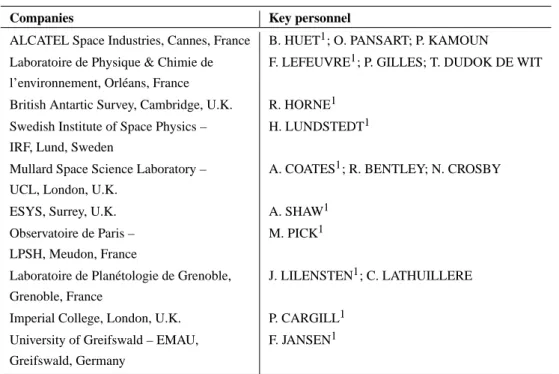
This paper has been written from the work package enti-tled “Space Weather Parameters”, prepared as part of a study conducted by the consortium lead by ALCATEL Space & LPCE (France) in the frame of an ESA contract aiming at the definition of an European Space Weather Programme. All work packages have received the contribution from the dif-ferent consortium members (see Annex 1 for a presentation of the consortium). A parallel study has been undertaken by another consortium led by the Rutherford Appleton Labora-tories (UK). Among the tasks of the consortium was to define the parameters and the associated measurements, which are necessary to describe and monitor the Sun-Earth system in the space weather context.
Space weather can be considered from two different stand-points, the numerical modelling of the whole system on the one hand, and the needs of the users, i.e. monitoring and forecasting the values of some specific quantities, on the other hand. Our approach has been to start with a review of the modelling effort, which is presented in this paper.
The driving source of the Solar Terrestrial phenomena is the Sun’s magnetic field. The related magnetic energy is con-verted into thermal and kinetic energy, and gives rise to elec-tromagnetic and particle solar radiations. The plasma that is ejected from the upper solar atmosphere is accelerated to su-personic speeds, and the Sun’s magnetic field lines are frozen
in the plasma. The Earth’s magnetic field behaves as a solid obstacle for the plasma. It gives rise to the magnetospheric cavity around which the solar wind flows, with energy and material exchange through the magnetosphere boundary. Fi-nally, both magnetospheric plasma and solar electromagnetic radiations interact with the Earth’s atmosphere, giving rise to the ionosphere and thermosphere. This very short sum-mary shows that the entire Solar-Terrestrial system can be described and understood in terms of a succession of sub-systems that exchange material and energy: the Sun’s atmo-sphere, the interplanetary medium, the magnetoatmo-sphere, and finally, the ionosphere-thermosphere system. Figure 1 shows a schematic description of the solar-terrestrial phenomena in terms of the interaction between these sub-systems.
The elucidation of the physical processes involved in each sub-system, and in the interaction between any two of them, is an important key in any space weather program. Our un-derstanding of the whole Sun-Earth system is, however, still incomplete, although research and operational models are available. There exist research models for each sub-system, but their maturity is very different, depending on the com-plexity of physical phenomena and on the available observa-tions. Operational models have already been developed only for some sub-systems. Our aim is not to present an exhaus-tive list of models but rather to give a comprehensive picture of the modelling effort of the different scientific communities concerned by space weather.
We have chosen to organise our presentation by classifying for each sub-system the models in two main classes:
– the empirical models that characterise the relations
be-tween relevant parameters from available observations;
– the physical models that describe a given sub-system on
the basis of quantitative laws between relevant param-eters. Contrary to the empirical models, the relations between parameters are expressed in terms of a priori known physical laws, with relevant simplifications, if any. They are expressed as a set of partial derivative equations, with coefficients to be estimated.
Recently developed space weather models based upon arti-ficial techniques, such as neural networks genetic algorithms and expert systems, are not presented here, nor are the tech-nological models which estimate the specified effects of our environment on a given “system”, for example, those dealing with radiation doses, spacecraft charging, proton fluences or atmospheric drag.
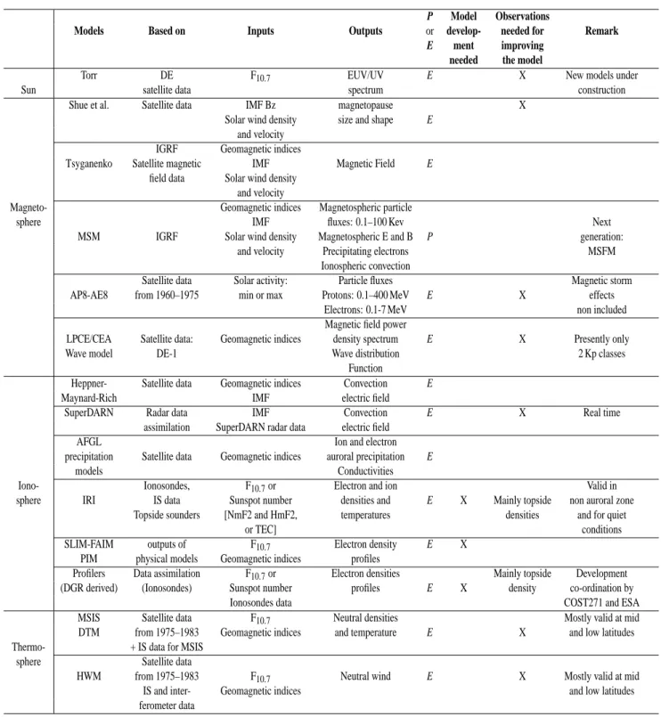
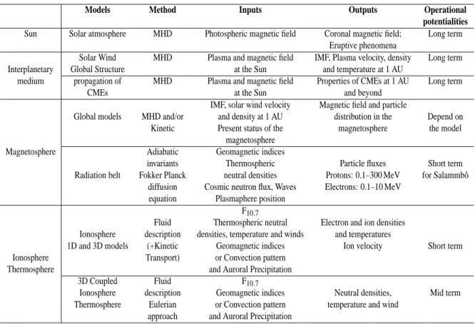
In this paper, we consider successively the different sub-systems that are involved in solar-terrestrial relations: the Sun, the interplanetary medium, the magnetosphere, and the ionosphere-thermosphere system. The last section of the pa-per presents a model synthesis, by means of tables that line their main characteristics, including their input and out-put parameters.
2 The Sun
Most of the structures and phenomena present in the solar at-mosphere – in particular eruptive phenomena, such as flares and coronal mass ejections (CMEs) – result from the pres-ence of a dominant magnetic field. Eruptive events corre-spond to a liberation of magnetic energy stored in the solar corona. This energy is then converted into:
– heating of the environment associated with UV/EUV
and X beams;
– particle accelerations (electrons and ions) associated
with an X emission when those particles interact with the environment;
– movement of matter.
Solar flares correspond to localised phenomena covering at most a few percent of the surface of the Sun, while CMEs are larger scale phenomena that can involve a non-negligible part of the Sun’s global configuration. Those may have different origins and associated events, such as global magnetic non-equilibrium or prominence disruption.
The global solar atmospheric models are developed mainly in the framework of Magnetohydrodynamics (MHD). The relevant set of equations describes the interaction of ionised coronal plasma with the coronal magnetic field in the pres-ence of the plasma pressure and gravity forces. These models may be presented in the context of space weather, although they are still essentially used for theoretical purposes. The associated numerical codes are mostly research tools due to the actual state of the art in solar MHD modelling. We present thereafter two main classes of complementary mod-els used for different purposes: the static modmod-els for equilib-rium reconstruction of the solar coronal magnetic field and the dynamic models to describe its evolution:
– the first class of models arises from the impossibility of
measuring the coronal magnetic field. The structure of the active regions should be estimated before an erup-tive event, in order to determine the intrinsic properties of the magnetic configuration. Thus, one has to recon-struct the coronal magnetic field and, therefore, to solve the equations of the solar atmospheric physics when the boundary conditions are the values of the magnetic field measured in the colder photosphere by vector magne-tographs;
– the second class of models aims at studying the
dynam-ical evolution of the active regions. The energy storage and energy release in these regions, as well as their sta-bility, are described from the evolution of the magnetic configurations which are constrained by a driver whose origin may be sub-photospheric (emerging flux), photo-spheric (boundary motions) or coronal (interaction with other active regions). These models solve – to a certain extent – the full MHD equations.
C. Lathuill`ere et al.: From the Sun’s atmosphere to the Earth’s atmosphere 1083
Fig. 1. Main physical processes that act on space weather (Dudok de Wit, personal communication, 2001).
Both classes of models are complemented by a whole set of boundary conditions which then define a set of boundary value problems.
2.1 Reconstruction and study of the active region static structures
Equilibrium reconstruction of the coronal magnetic field above active regions using photospheric magnetic data has been the subject of numerous studies since the first attempts (Schmidt, 1964). They may range from observational prob-lems, such as those related to the 180◦ambiguity resolution, which remains on the transverse component of the photo-spheric magnetic field, to crucial theoretical problems related to the nature and the determination of the correct type of boundary conditions that have to be used in order to avoid an ill-posed problem, as was the case for a long time. Details and numerous relevant aspects of these studies are discussed in Amari and D´emoulin (1992) and Amari et al. (1997).
In an active region, prior to any eruptive event, typical time variations are so small that one can then solve the MHD equations under static hypothesis. The coronal magnetic pressure is much larger than the gas one, and gravity can be neglected outside prominences. This is the so-called force-free approximation. This is equivalent assuming that at any point the current density and the magnetic field are parallel. The proportionality factor α(r) and the magnetic field are de-termined by the boundary conditions defining the boundary value problem.
In the regions of higher density, the plasma pressure gra-dients and the gravity have been included. This can be done self-consistently in full MHD methods or more qualitatively by seeking magnetohydrostatic solutions of the MHD equa-tions.
2.1.1 Current free (potential) model
The simplest physical approximation is the so-called “cur-rent free” approximation (α = 0), which only requires the longitudinal photospheric component of the magnetic field as a boundary condition. It was first considered by Schmidt (1964) and is currently routinely used in most of the terres-trial solar physics centres, on the basis of observations (Saku-rai, 1989). It is also used as the initial conditions for funda-mental MHD studies dealing with synthetic problems. This kind of reconstruction is performed following a Green func-tion approach or using a Laplace solver to compute a poten-tial scalar function and the associated magnetic field (Priest, 1982).
2.1.2 Linear force-free model
The zero-current approximation does not apply to many ac-tive regions that have a magnetic energy above the minimum energy, which corresponds to the current free field for the same distribution of the vertical distribution of the photo-spheric normal magnetic field. The first step towards a more realistic modelling consists of considering a nonzero, but constant α that allows one to introduce coronal electric cur-rents. Different methods exist that use the longitudinal com-ponent of the magnetic field. They are based on Green func-tions (Chiu and Hilton, 1977) or Fourier transform (Alissan-drakis, 1981), with the latter currently used (Demoulin et al., 1997). Following the general approach of Low (1992), this linear constant-α Fourier method has been extended to take into account gravity and pressure forces by means of a linear computational program (Demoulin et al., 1997; Aulanier et al., 1998).
Although they suffer from several limitations (see be-low), linear models can be used for some classes of prob-lems (topology, prominence) in moderately sheared struc-tures. Their main advantage remains the weak computational resources they need and their computational speed for the current free approximation, which explains why they could be used routinely in a space-weather program.
2.1.3 Nonlinear force-free model
As for the reconstruction without current, several limitations exist regarding the use of the linear reconstruction model:
– the solutions correspond to a minimisation problem for
the energy, constrained by the normal component of the magnetic field and by the total magnetic helicity, induc-ing a limited amount of available magnetic free energy;
– the electric currents cannot be locally intense, while
the observations show very clearly important localised shear concentrated along the inversion line of the nor-mal component of the photospheric magnetic field. The only hope of incorporating large localised electric cur-rents is to assume that the configuration is in a nonlinear force-free state, that is to say that α (which now depends on the position r) is also an unknown of the problem. Different types of boundary conditions define different boundary value problems and codes:
– a first relatively natural method consists of imposing the
three components of the magnetic field B measured at the photospheric level. The problem amounts to pro-gressively extrapolating the data step by step toward the corona. This is the vertical integration method intro-duced by Wu et al. (1990). However, this method is based on a mathematical formulation associated with an ill-posed boundary value problem. This lead to an exponential divergence, which limits the reconstruction at low altitudes. Some methods have been proposed in order to avoid this divergence (Cuperman et al., 1990; Demoulin et al., 1992). Other attempts have been made to regularise the linear version of this method (Amari et al., 1998);
– a second class of reconstruction methods is based on a
well-posed formulation, which corresponds to observed boundary conditions that imply:
– the normal component of the photospheric
mag-netic field (in the local system of reference asso-ciated with the Sun);
– α at the photospheric level, when the sign of the
normal component Bz of the measured magnetic
field has a given a priori value: as an example, α is set in the areas where Bzis positive and then
com-puted through transport along the magnetic field lines to the photospheric zones where Bz is
nega-tive.
This kind of mathematical formulation was introduced by Grad and Rubin (1958) and consists of a decompo-sition of the nonlinear problem in two sets of elliptical (for the magnetic field) and hyperbolic (for α) problems. It gives rise to two types of numerical codes, which cor-respond to the Lagrangian and Eulerian approaches:
– Sakurai (1981) uses a Lagrangian approach for each
field line. He injects progressively the photospheric electric current on each field line;
– Amari et al. (1997) use a global approach in order
to solve the elliptical and hyperbolic problems. The corresponding codes with their different versions constitute the EXTRAPOL code.
These two codes, localised in Japan and in France, are used to reconstruct the configurations of the active re-gions coming from MITAKA data for the Japanese ver-sion and from Hawaii (HSP, IVM) and Boulder (ASP) for the French one. The local Lagrangian approach (Japan) seems to imply a more important limit for the reproducible maximum shearing than the Eulerian ap-proach (France);
– a third class of methods is based on solving the MHD
equations, injecting the vertical component of the elec-tric current and imposing the normal component of the magnetic fields as photospheric boundary condi-tions. The system relaxes toward a state which corre-sponds to the observed values. This method is called the “resistive-relaxation” method. It was introduced by Mi-kic and Linker (1994) and was also implemented in the French METEOSOL MHD-research code. Although the mathematical justification for this method is not yet clear, the corresponding codes have been used on real cases with relatively good success;
– another method is still at a very experimental state
of development. It is the “weighted residue method” (Pridmore-Brown, 1981). This method minimises two residuals: one is associated with the magnetic force, and the second one is associated with the difference between the directions of the photospheric transverse components of the computed and observed magnetic fields. This method has been used only in theoretical situations corresponding to fictive periodic data;
– finally, a method called “constraint and relaxation
method” (Roumeliotis, 1996) consists of two repeated steps:
– impose on the vector potential the minimisation of
the difference between the computed and observed transverse components;
– relax toward an equilibrium state, using a relaxation
code which incompletely solves the MHD equa-tions,
Table 1. A synthesis of MHD codes for the evolution of the solar magnetic configurations Laboratories Characteristics Aims San Diego (USA) 2.5D, 3D coronal MHD
Finite differences (Mikic and Linker, 1994) Semi-implicit
NRL et NASA (Wash. DC) 2.5D, 3D Coronal and internal MHD (De Vore et al., 2000) Spectral + finite volumes
Explicit
Boundary conditions (. . .)
Japan NAO/Mikata 2.5D, 3D Chromospheric and internal (Matsumoto et al., 1993) Explicit MHD
artificial viscosity anomalous
Observatoire de Meudon 2.5D, 3D coronal MHD Ecole Polytechnique (France) differences and finite volumes
(Amari et al., 2000) (semi) and implicit
Strasbourg (France) cylindrical coronal MHD (Baty and Heyvaerts, 1996) Boundary conditions stability Pisa / Firenze (Italy) cylindrical (3D) San Diego coronal MHD (Lionello et al., 1998) 2D reduced MHD turbulence Nice (France) 1D, 2D Turbulence (Galtier et al., 1997) Finite differences, Spectral Intermittence Argentina Reduced MHD (2D+) Turbulence (Dmitruk et al., 1998) Cartesian Flare-heating
Spectral (Fourrier)
University of Michigan (USA) 2D, 2.5D, 3D (?) Comets – wind (Israelevich et al., 2001) Roe scheme astrophysics
Finite volumes
NCSA (Illinois) 2.5D, (3D ?) Astrophysics (Stone and Norman, 1992) Finite volumes laboratories
Van Leer, PPM
DAEC + DESPA (France) cylindrical /(Spherical 2.5D) Dynamo + wind (Grappin et al., 2000) Z-periodic laboratories
Spectral – Finite differences
Chicago (USA) cartesian Astrophysics (Fryxell et al., 2000) laboratories
This method has been tested with encouraging results on a theoretical case, as well as on an observed active region. 2.2 Evolution of the magnetic configurations
As far as the evolution of the magnetic configurations is con-cerned, the MHD codes belong to the domain of research even more than the reconstruction codes. It concerns the fundamental numerical research for the codes themselves: boundary conditions, geometry, temporal scheme, mesh def-inition, etc., but also the fundamental solar physics. The ob-jective is to elucidate the fundamental mechanisms that gov-ern the eruptive phenomena: flux emergence, energy storage,
influence of the photospheric movements such as differential rotations or magnetic reconnection, etc.
The existing codes depend on the different classes of prob-lems they address: there is no universal MHD code, in the same way as there is no universal telescope. However, it will still be a long time before the MHD codes can be used for space weather purposes, in order to test the stability of the magnetic configurations in active regions. These regions may be first reconstructed by using an equilibrium reconstruction code. This is the approach followed by some groups.
The existing world wide codes can be distinguished by the following characteristics:
– dimension: 2D, 2.5D, where the vectors have 3
compo-nents but only depend on 2 space variables, 3D;
– geometry: spherical for the global models, Cartesian
for the description of the active regions at local scales, cylindrical for more specific problems, such as the sta-bility of the coronal loops or of the coronal heating;
– numerical scheme and space digitisation: finite
ele-ments, finite volumes, spectral methods, collocation, etc.
– physical approach: heating, resistivity, solar wind
in-clusion facing the particularly important and difficult problem of breakdown of the MHD approximation. Table 1 only attempts to synthesize these different ap-proaches worldwide. We are aware that on-going work may give rise to new codes in the near future. We only show here the codes and the associated developing groups and give only one reference per group, as a starting point. The more nu-merous groups that only use the codes are excluded from the table.
3 The interplanetary medium
The solar wind is a prominent part of the Sun-Earth system that is difficult to model because observations are difficult and often indirect. The solar wind corresponds to the outflow from the upward solar atmosphere of the coronal plasma, heated up to several million K. Its speed ranges between 250 and 950 km.s−1 at the Earth’s orbit (1 AU). It is structured by the Sun’s magnetic field lines frozen in the flow. The so-lar wind interacts in the interplanetary medium with galactic cosmic rays. Since the solar wind expansion does not occur in a vacuum but in an interstellar space filled with neutral and ionised gases, galactic cosmic rays and galactic mag-netic fields, the region where the solar wind dominates is limited by the heliospheric boundary – a region where the energy densities of the solar wind and the interstellar space are equal. This boundary is located between about 50 and 100 AU.
3.1 Solar wind modelling
The main structures or regions present in the solar wind are:
– the high velocity solar wind, associated with the coronal
holes;
– the low velocity solar wind;
– the regions of interactions between high and low
veloc-ity solar winds;
– the heliospheric current sheet;
– the signatures in the interplanetary medium of the
CMEs, associated or not associated with shocks. In practice, these signatures are observed at large distances from the Sun near the Earth or the Lagrange point L1.
The influence of the solar wind results from both its very structure and its interaction with the propagation of solar per-turbations, such as energetic particles resulting from solar eruptions or interplanetary shocks or CMEs. The structure of the interplanetary magnetic field lines, which drives the particle propagation, may, in given situations, dramatically affects this propagation and, therefore, the resulting effects at Earth. This ambivalent action can be illustrated by ex-amples of major events at the Sun with minor effect’s at the Earth, or on the contrary, minor events at the Sun resulting in a major perturbation at the Earth.
Solar wind models have been developed to address many aspects of its structure. Fairly simple models can be devel-oped by treating the solar wind from a hydrodynamic point of view, and thus solving the one-dimensional equations of mo-tion along a single field line (e.g. Parker, 1963). The main aim of such models is to obtain accurate expressions for the plasma density, velocity, and especially temperature at 1 AU. They are also amenable to adding multiple ion species and to including quite detailed calculations of different ionisa-tion states and even the effect of plasma instabilities on the temperatures.
However, from the point of view of space weather, it is the large-scale multi-dimensional MHD models that are the most relevant. One class of these models examines the global structure of the solar wind plasma and magnetic field in the heliosphere. These models are quasi-steady state, but incorporate solar rotation, and a three-dimensional mag-netic field. For solar minimum conditions – for which they are best suited – they clearly demonstrate the formation of the familiar co-rotating interaction regions at distances of 1 AU and beyond (Pizzo, 1982, 1991). The Ulysses mission has permitted a comparison of these results with the three-dimensional solar wind structure. The agreement is good, especially in terms of plasma flows upward and downward from the ecliptic plane (Riley et al., 1996).
A second family of models deals with the motion of coro-nal mass ejections in the solar wind. The goal is, for given plasma and magnetic field conditions at the Sun, to calcu-late the properties of the CME at 1 AU and beyond. Early models treated the CME as a pressure pulse, but these are now viewed as irrelevant. Other purely hydrodynamic mod-els have been developed by Riley and collaborators during an investigation of so-called over-expanding CMEs. They showed that with a large plasma over-pressure at the Sun, the conditions observed by the Ulysses spacecraft at large dis-tances could be roughly reproduced (Riley et al., 1997).
The most geo-effective type of CMEs are magnetic clouds. Models for these have been developed by a number of groups who have – in general terms – established that magnetic clouds can propagate from the Sun to the Earth while re-taining their organised magnetic structure (e.g. Cargill et al., 2000; Odstrcil and Pizzo, 1999; Vandas et al., 1996). The clouds interact with the solar wind by two processes. First, the cloud magnetic field can undergo magnetic reconnection with the solar wind field, leading to its ultimate destruction at large distances. Second, the interaction of the cloud with the
solar wind plasma leads to considerable changes in its shape, as well as leading shock waves. This modelling is plagued by difficulties in initialising the solar wind magnetic field in a way that minimises errors in the divB = 0 condition. Proper 3-D modelling actually requires that this problem be resolved. Further discussion of such CME models can be found in Cargill and Schmidt (this issue).
Among the empirical models, one can quote Wang-Sheeley, based upon the discovery of an anti-correlation be-tween the solar wind velocity and the rate of expansion of the magnetic flux tubes (Wang and Sheeley, 1992). The model is based on observations of magnetographs at the Sun’s surface and on deduced maps of coronal holes, surface magnetic field sources and solar wind velocity. It forecasts the IMF polarity and the solar wind velocity at the Earth, two parameters that are mandatory for geomagnetic activity forecasting1. 3.2 Solar wind – cosmic ray interaction
Cosmic rays at the Earth are high energy particles – from 500 MeV to about 1012GeV – insensitive to the magneto-sphere state. The main components are protons, electrons and light nuclei. Below about 1 Ge V/nucleon, the cosmic ray flux is strongly decreased due to adiabatic deceleration with the solar wind, which results a decreasing flux below this energy at the Earth’s orbit. The intensity of the cosmic rays on the Earth maximises when solar activity is minimal (quiet Sun) and minimises vice versa (active Sun), with an average variation in intensity of about 20%.
Models describing the propagation of the cosmic rays through the solar wind are based on a second order equation whose main input parameters are the solar wind characteris-tics and the interplanetary magnetic field. Fisk et al. (1998) show that most of the observed phenomena can be accounted for within acceptable ranges of these parameters. However, no single model, with a single choice for the input param-eters, has been able to account for all the observed features of galactic and anomalous cosmic ray behaviour. The most highly developed models concern the interpretation of long-term variations of the flux of cosmic rays at the Earth.
4 The magnetosphere
The magnetosphere is the region of the ionised environment of the Earth where the Earth’s magnetic field has a dominant control over the motion of charged particles. The bound-ary layer between the magnetosphere and the solar wind is the magnetopause, at which the dynamic pressure of the so-lar wind is balanced by the magnetic pressure of the Earth’s magnetic field2. The location of the magnetopause obviously
1http://solar.sec.noaa.gov/∼narge/
2The dynamic pressure of the solar wind is 2ρV2cos2χ, where ρand V are the solar wind density and velocity, and χ is the an-gle between the direction of the solar wind velocity and that of the normal to the magnetopause; the magnetic pressure of the Earth’s magnetic field is B2/2µ, where B is the tangential component of
depends on the status of the solar wind. Under typical solar wind conditions, the terrestrial magnetosphere extends up to
∼10 Earth radii (RE) in the sunward direction and to several
hundreds RE in the antisunward direction. The solar wind
velocity is supersonic at 1 AU, and the magnetosphere be-haves as a solid obstacle. Therefore, there is a bow shock upstream from the magnetopause. In the solar direction, the bow shock is located at a distance in the range of 2–4 RE
from the magnetopause. The region between the bow shock and the magnetopause is the magnetosheath, in which the shocked solar wind plasma has a lower velocity and a tem-perature 5 to 10 times higher than in the solar wind.
The inner magnetosphere is the region of major concern for space weather issues. Three regions have been identified there following different criteria: the plasmasphere, the radi-ation belts, and the ring current:
1. the plasmasphere corresponds to a cold (Te≈1 eV) but
dense (ne ≈ 5 × 102cm−3) plasma which co-rotates
with the Earth. It is a torus-shaped volume in the inner-most magnetosphere. The outer boundary of the plas-masphere is the plasmapause, where the density sharply drops down to about 1 cm−3. On average, the
plasma-pause is located about 4 RE in the equatorial plane, i.e.
a McIlwain parameter3 L = 4. It may reach out to
L =5 − 6 during periods of magnetospheric quietness and be compressed down to L = 3 during periods of intense magnetospheric activity;
2. the ring current refers to “those parts of the particles in the inner magnetosphere which contribute substantially to the total current density” (Hultqvist et al., 1999). It is then defined with regard to its magnetic signa-ture, and corresponds to a toroidal-shaped electric cur-rent that flows westwards around the Earth, with vari-able density at geocentric distances between ∼ 2 REand ∼9 RE. During magnetospheric storms, the particles
that contribute substantially to the total current density are mainly trapped ions in the medium energy range (few tens of keV to few hundreds of keV) that origi-nate in the solar wind (He++), the plasmasphere and the ionosphere (O+). During low activity periods, the
particles responsible for the ring current are mostly pro-tons. This change in composition impacts the evolution with time of the ring current, because loss mechanisms (wave-particle interactions, charge exchange, Coulomb collisions, etc.) depend on the mass and energy of the particles;
3. the radiation belts generally refer by now to the “high energy ions and electrons that can penetrate into space-craft shielding materials and eventually cause radiation damage to spacecraft instrumentation and to humans”
the Earth’s magnetic field at the magnetopause. µ is the magnetic permeability of the medium.
3For a given geomagnetic field line, the Mac Ilwain parameter Lis the geocentric distance of the point where it crosses the mag-netospheric equator. It is expressed in Earth radii (RE).
(Hultqvist et al., 1999). The radiation belts are defined with regard to the energy of particles trapped in the geo-magnetic field lines, above ∼ 100 keV and reaching val-ues of hundreds of MeV. Most of the trapped particles are protons and electrons, giving rise to the proton and electron radiation belts:
– the proton belt has generally one maximum, which
corresponds to a McIlwain parameter L that de-creases with increasing proton energy. For 1 MeV, the maximum corresponds to L ∼ 2.5 (i.e. field lines crossing the equatorial plane at an altitude heq
of ∼ 10 000 km), while it corresponds to L ∼ 1.4 (i.e. heq ∼ 2 500 km) for 50 MeV. The proton
belt is fairly stable. At low altitude, it is mod-ulated by the solar cycle, in particular in the re-gion of the South Atlantic magnetic anomaly: its intensity is maximum during solar minimum, and minimum during solar maximum. Major magnetic storms (e.g. March 1991) may significantly impact the proton belts, in particular for high McIlwain pa-rameters values;
– the electron belt has generally two maxima,
giv-ing rise to the internal and external electron belts. The internal belt, with a maximum corresponding to 500 keV around L ∼ 1.4 (i.e. heq ∼6 400 km),
does not significantly vary with time. On the con-trary, the external belt, the maximum of which is around L ∼ 4 (i.e. heq ∼ 19 000 km) fluctuates
dramatically under the control of strong magnetic storms: short-term variations of the flux, up to 4 orders of magnitude in a few hours, can be ob-served during periods of intense magnetic activity. The long-term variation of the external belt fluxes is driven by the solar cycle: the annual mean values of the flux are maximum during the descending phase (about 3 years after the maximum), when coronal holes are in good conjunction with the Earth.
It is worth noting that ring current, radiation belts and the plasmasphere partially overlap. For instance, at L = 3, the density of the cold plasma is about 1000 times higher than the density of energetic protons (> 100 keV), whereas the energy density of energetic protons dominates by a factor of about 1000. It is also worth noting that trapped radiation belts and the ring current are actually closely related, since the major part of the ring current is carried by trapped par-ticles and all the trapped parpar-ticles contribute to the ring cur-rent (Hulqvist et al., 1999). For a thorough description of the present knowledge on these regions of the magnetosphere, refer to the recently published reviews on the ring current (Daglis et al., 1999) and the inner magnetosphere (Hultqvist et al., 1999).
4.1 Global magnetosphere modelling 4.1.1 Empirical models
Empirical models for the bow shock and magnetopause have been developed for decades, in the case of the Earth, as well as that of other magnetised planets (e.g. Slavin and Holzer, 1981). Shue et al. (1997) recently published a well docu-mented model, based on fresh data. It has a simple functional form driven by two adjustable parameters: the stand-off dis-tance in the solar direction and the tail flaring.
Empirical models for the magnetic field inside the magnetosphere are based on a statistical analysis of the avail-able magnetic field observations, parameterised by geomag-netic indices. They rely basically on a combination of the Earth’s planetary magnetic field – usually described by the IGRF model – and external fields estimated from both in situ magnetic field measurements and mathematical mod-elling of the current systems (e.g. Tsyganenko, 1990; 1995; Hilmer and Voigt, 1995). These models are updated contin-uously to account for more and more complex processes in the magnetosphere.
At a given time, the dynamics of the magnetosphere depends on both the present solar wind conditions and magnetosphere status. This status, therefore, depends on the past history of the magnetosphere, and models that only use the present magnetic field values as input cannot provide re-liable predictions of the magnetospheric state. In order to develop better predictors, indicators of the magnetosphere history should be added to the inputs.
4.1.2 MHD simulations
Fully three-dimensional MHD models of the magnetosphere have already been developed for scientific use. Their in-put parameters are typically solar wind density, velocity, and interplanetary magnetic field. The inner boundary of the magnetosphere is typically set at somewhat above 3 RE,
and physical quantities are mapped down to the ionosphere along field lines. The output is the dynamic response of the magnetosphere-ionosphere system. These models do not generally provide a proper description of the inner magneto-sphere, because of (i) the definition of the inner boundary, and (ii) the presence of dominant non-MHD processes in the inner magnetosphere.
This field is very active. Several groups are develop-ing their own model, and have not yet published their re-sults. The situation is then expected to evolve rapidly during the next decade. The best known global MHD models of the magnetosphere are those developed at the University of Maryland (see Mobarry et al., 1996) and at the University of California at Los Angeles (see Raeder et al., 1997 for a recent application). Another model developed at UCLA (Walker et al., 1993) is worth being mentioned here. In Europe, a model is currently been developed for scientific use only at the Finnish Meteorological Institute (Janhunen, 1996).
4.1.3 Kinetic models
The behaviour of the inner magnetosphere cannot be de-scribed in the frame of the MHD approximations4. Models of the inner magnetosphere should take into account:
– the non-local character of the plasma response for any
transport with characteristic time duration longer than the shorter reflection period;
– the effect of the plasma on the magnetic field;
– the interaction between the different waves in the
plasma.
Self-consistent kinetic methods properly describe the field-particle interaction and satisfy these requirements at the ex-pense of very heavy calculations. An example of such an approach is the model of substorm growing phases recently developed by Le Contel et al. (1999a, b). Their model is based on the approach proposed by Pellat et al. (1994) and Hurricane et al. (1995) to describe electromagnetic perturba-tions in a non-adiabatic5plasma. It allows one to estimate the adiabatic response of the plasma to a given external elec-tromagnetic perturbation that originates in the solar wind: an east-west current flowing close to the equatorial plane in the far tail.
The computations could become significantly simpler if one neglects the perturbation generated by the motion of par-ticles, which assumes that the magnetic field model used takes into account satisfactorily the existence of the currents associated with the particles whose motion is studied. This approach uses both an Eulerian approach (global model of the magnetosphere) and a Lagrangian one (particle trans-port). In practice, it provides an efficient tool for describing the trajectories of the particles in the magnetosphere once an accurate model of the magnetospheric magnetic field, for example, Smets (1998) used such an approach to study the particle distribution functions associated with reconnection processes. Numerical simulation of particle transport then allowed him to characterize particle distributions associated inside the magnetosphere to reconnections at sites with dif-ferent topology and localisation.
4The ideal MHD basically assumes that the plasma is a perfectly
conductive medium.
5Adiabatic responses of a plasma correspond to situations where
the motion invariants defined in the frame of the Hamiltonian me-chanics are conserved. For a charged particle in the presence of a magnetic field, the first invariant is its magnetic moment µ, the sec-ond invariant is the integral along the field line of the component along the magnetic field of the particle momentum, and the third one is the magnetic flux encircled by the particle’s periodic drift shell orbits.
4.2 Specific models
4.2.1 The Magnetospheric Specification and Forecast Model (MSFM)
The MSFM (Freeman et al., 1994; Lambour et al., 1997) is a large-scale physical model designed to specify fluxes of elec-trons, H+, and O+in the energy range responsible for
space-craft charging, ∼ 100 eV to ∼ 100 keV. It is being developed for operational use by the US Air Force, and it is probably, at present, the closest to being an operational large-scale physi-cal model. Its description is available on the net6. It is an up-date of a series of earlier models. Its predecessor, the MSM (Magnetospheric Specification Model), is routinely used by NOAA/SEC for space weather services. Its major improve-ment compared to the earlier models, is the complexity of the electric and magnetic field models and its capability to run in real time.
The primary input parameters for MSFM are: 1. the Kpand Dstgeomagnetic indices;
2. the polar cap potential drop and the auroral boundary in-dex that specify the polar ionospheric electric field dis-tribution and the auroral precipitation pattern;
3. the solar wind density and speed, and the interplanetary magnetic field (IMF).
Secondary input parameters include: 1. the sum of Kp;
2. precipitating particle flux and polar cap potential pro-files from the operational DSMP satellites.
The solar wind density and speed define the magnetopause stand-off distance, and the IMF is used to select the approate convection pattern in the polar cap. All together, the pri-mary input parameters determine the electric and magnetic field models used. The sum of Kpis used as an indicator of
the long-term activity level.
The model can operate with reduced sets of input parame-ters, and in particular, with Kpalone. It also includes neural
network algorithms that predict the input parameters from solar wind measurements. Thus, it has some capability for short-term space weather forecasting.
MSFM follows particle drift through the magnetosphere using slowly time-varying electric and magnetic field mod-els. The electric and magnetic field configurations are up-dated every 15 min. The particle distribution is isotropic, and the model keeps track of energetic particle loss by charge ex-change and electron precipitation into the ionosphere.
MSFM successfully accounts for most major electron flux enhancements observed at geosynchronous orbit. Flux dropouts that often precede the flux enhancements are pre-dicted with less confidence, and they are often missed near the dawn meridian.
4.2.2 Ring current models
It has already been mentioned that the ring current compo-sition and dynamic particles is driven by the level of the magnetospheric activity. During periods of magnetospheric activity, the ring current dynamics is driven by particle in-jection: direct ionospheric ion injection, inward transport of plasma sheet and pre-existing ring current particles. On the contrary, the behaviour of the quiescent ring current is driven by diffusion of low energy protons in the presence of con-vection electric fields (see, e.g. Daglis et al., 1999). Differ-ent quantitative models have been developed accordingly for storm- and quiet-time ring currents.
A family of storm-time ring current models neglects direct injection of ions from the ionosphere. The main source of ring current particles is then the plasma sheet, and the char-acteristics of that source enter the models as boundary con-ditions. At least four groups are working at present along this path. They are located at the University of Michigan, the Aerospace Corporation, NASA-Goddard Space Flight Cen-tre, and Rice University (see Chen et al., 1994 for a review of these works). Differences between their models are mainly related to a different selection of aspects of the problem that are treated at a state-of-the-art level or neglected. One of the main difficulties for these models in the context of space weather operational use is the specification of the boundary condition (i.e. the distribution function of the particles at all parts of the boundary, where the drift velocity is inward) in absence of adequate real-time data.
More sophisticated simulations have been developed, which involve both global magnetospheric models and La-grangian models of particle transport. They have been de-veloped to address questions in relation to academic research rather than to space weather activities. Such a coupled in-vestigation is, however, very promising for space weather activities, since it provides an efficient tool for the particle distribution function determination in a given region of the magnetosphere.
With the objective of analysing the ring current dynam-ics, Fok et al. (1993) have developed a kinetic model that simulates the evolution with time of the distribution func-tions for the dominant ions (H+, He++, O+), as a result of charge exchange and Coulomb collisions. Their results show that during the recovery phase of a magnetic storm, Coulomb collisions lead to generation of low energy (< 500 eV) ions and significant heating of plasmaspheric populations. More recently, the model of Fok et al. (1993) and the particle code of Delcourt et al. (1990a) have been coupled to investigate the ring current response to the field line depolarisation ob-served in the inner magnetosphere during the substorm grow-ing phase. The code of Delcourt et al. (1990a) computes the path of charged single particles, given time-varying elec-tric and magnetic fields, from their injection in the magneto-sphere – from the magnetosheath or the ionomagneto-sphere – to their input in the plasmasphere.
In a more recent study, Fok et al. (1999a) used the parti-cle code of Delcourt et al. (1990b) to estimate the partiparti-cle
distribution in the near tail (at a geocentric distance of about 12 RE), by means of back propagation of particles to their
sources. The transport and acceleration of these ions in the inner magnetosphere, as well as their contribution to the ring current, are then computed using the kinetic model of Fok et al. (1993), with a magnetic field more realistic than a dipo-lar one. These simulations account for many characteristic features of substorms. Further refinements of these investi-gations will involve an estimate of the initial particle distri-bution functions from the results of MHD simulations (see, e.g. Fok et al., 1999b) for given solar wind situations, instead of semi-empirical modelling.
Understanding the loss process in the region where the hot ring current plasma coexists with cold plasmaspheric plasma requires modelling of the interaction between ring current ions and plasma waves resonantly generated by the coexist-ing hot and cold plasmas. Modellcoexist-ing wave particle interac-tion on a global scale is very challenging because it needs a self-consistent description of wave and particle behaviour.
4.2.3 Radiation belt models
4.2.3.1 Empirical models
Very early in the space era, it became clear that the average radiation doses received by satellites are key parameters that should be known. The United States and the former Soviet Union, therefore, started building empirical models of radi-ation belts, using data collected for several years on board a number of satellites.
In the United States, these models were developed for NASA by Aerospace Corporation. The latest versions are the AP8 (Aerospace Protons #8) and AE8 (Aerospace Pro-tons #8) models (Sawyer and Vette, 1976; Vette, 1991). They have been built at the end of the 1970s, using data from about 40 satellites that were in orbit between 1961 and 1977, a pe-riod that mostly corresponds to solar cycle #20. They provide proton flux for energy in the range 100 keV to 400 MeV and electron flux for energy in the range 40 keV to 7 MeV, for altitudes up to that of geostationary orbits.
The necessity of updating these models led the United States to launch a satellite dedicated to radiation measure-ments: the NASA/DoD CRRES (Combined Release and Ra-diation Effect Satellite) satellite. It has been operational for 14 months – between August 1990 and October 1991 – that roughly corresponds to the maximum of solar cycle # 22. The CRRES data have been used by DoD to develop new empirical models for the proton (CRRESPRO) and electron (CRRESELE) radiation belts (see, e.g. Brautigham et al., 1992; Gussenhoven et al., 1993). These models do not pro-vide a significant updating of earlier models, because (i) the altitude and energy ranges they cover are not as wide as those covered by NASA’s AP and AE models, and (ii) they rely on data collected by only one satellite during a disturbed period that is probably not representative of the average behaviour of the radiation belts.
On the contrary, the durability of some meteorological satellites gives the opportunity to improve the models for the low altitude range. Boeing is presently preparing for NASA a model using the NOAA/TIROS satellite data (Huston et al., 1998). This model relies on measurements made since 1978, i.e. over almost two solar cycles. Despite its limitation with respect to altitude (< 800 km) and energy (3 ranges for energy larger than 16 MeV), it is a significant improvement compared to earlier models because it describes the evolution with solar cycle of high energy proton fluxes. The authors are now trying to extend the altitude range addressed by the model.
In addition to the models described above, nucleus of models appear at many places in the world. Most of them rely on data from only one satellite, and their representative-ness is limited accordingly. As a result of these limitations, the AP8 and AE8 empirical models will probably still remain the standard to be used for mission planning during the next few years, despite their own limitations.
4.2.3.2 Physical models
Physical models have also been developed very early, in or-der to elucidate the radiation belt sources and their dynamics. Due to the limitation in the computer capacities, they did not significantly evolve during the 1980s. The increasing effi-ciency of computers allowed one to restart their development at the beginning of the 1990s. During the last few years, they allowed us to make possible significant breakthroughs in our understanding of the sources and dynamics of the proton and electron belts.
They rely basically on the resolution of the Fokker-Planck diffusion equation in adiabatic conditions. They take into account more and more different physical phenomenon:
– particle-particle interactions; – wave-particle interactions; – Coulomb interactions; – plasma influence.
An example of such code is Salammbˆo, a set of codes de-voted to the understanding of high energy charged particle transport in the inner part of the magnetosphere, in partic-ular during magnetic activity periods. The first one, called Salammbˆo-3D, solves the classical Fokker-Planck diffusion equation, either for proton or electron radiation belts, in the 3-D phase space. The equation is classically written in terms of the three adiabatic invariant, corresponding to energy, pitch angle and L McIlwain parameter, so this version is a real 2-D one in space, where the results are averaged with re-spect to the longitude (local time) (Beutier et al., 1995; Beu-tier and Boscher, 1995). The Salammbˆo-4D version is an extended version of Salammbˆo-3D, taking into account the longitude (local time), so it is a real 3-D one in space. It was developed to understand injections during substorm periods, and their effects, such as drift echoes or the growth of the
ring current. In this version, it is possible to follow particles in their drift around the Earth (Bourdarie et al., 1997).
Tests made on the prediction of the time dependence of the lifetime of trapped electrons (i.e. the time needed to have the initial flux decreased by a factor e) have shown that ra-diation belt models are very sensitive to the waves (Baus-sart et al., 2000). The elaboration of a physical radiation belt model, therefore, requires the introduction of a wave model. The two models presently used are the Abel and Thorne semi-empirical model (Abel and Thorne, 1998a, b) and the LPCE/CEA empirical model (Baussart et al., 2000; Lefeuvre et al., 2000) based mainly on statistics performed from 3 years of DE-1 data and on wave normal directions estimated from GEOS-1 and ISEE-1 data.
5 The ionosphere-thermosphere system
Above 90 km altitude, the upper thermosphere is character-ized by a large density decrease, that implies a decrease in the collision frequency between molecules. The temperature increases rapidly from about 180 K to the thermopause value of about 1000 K. This value, constant above 300 km, is also called the exospheric temperature. It is directly dependent on the solar energy in the UV and EUV bands and on the auroral energy inputs. The main atmospheric constituents, nitrogen and molecular oxygen, are dissociated and ionised by the absorption of EUV solar radiation and particle precip-itation to form the ionosphere. The resulting ionised species are mainly molecular ions (N+2 and O+2) at low altitude (be-low 200 km) and atomic ions (O+) at high altitude (above
200 km). N+ is created by N
2 dissociative ionisation, H+
by charge exchange reactions between O+ and H. Finally,
NO+arises from chemical recombination with neutrals. It is
a major ion of the E-region, although its neutral parent NO is a minor constituent of the atmosphere in that region. The ionosphere can, therefore, be said to be composed of three molecular ions (N+2, NO+and O+2), three atomic ions (H+, N+and O+) and electrons. The altitude of the maximum of the electron density is close to 250 km.
The understanding of the behaviour of this solar-terrestrial sub-system and its effects on technological operations is de-termined by the ability to model at least the height, geograph-ical and time distributions of the electron concentration and the neutral densities. The modelling effort has started a long time ago, due to the development of our technological soci-ety (telecommunications, orbitography, etc.). However, there is no numerical code or model that is able at the present time to describe accurately both the three-dimensional and time-dependent distribution of the ionospheric plasma, and the thermospheric densities during quiet and disturbed con-ditions. In other words, no model is able to reproduce in a satisfactory way both the climate and the weather of the Earth’s ionosphere-thermosphere. In addition, there is no well established experimental database that can be used to verify and test the existing models, in order to generate the improvements needed.
At present, most models are able only to reproduce con-sistently the climate of the ionosphere and the thermosphere, as defined mostly by diurnal, seasonal and solar cycle vari-ations. Serious theoretical and computational efforts, sup-ported by complex combinations of experimental techniques, are being done to model and predict the weather. This weather is defined as the hour-to-hour, day-to-day, week-to-week variability of the electron and neutral concentrations within the framework of the climatology.
Three different types of models can be identified, each of them having implicit limitations and advantages:
– semi-empirical and empirical models; – physical models;
– in the case of ionospheric modelling only, analytical
“profilers” based on routinely scaled ionospheric data. The physical models of the ionosphere and the thermo-sphere use as inputs results from empirical models of the convection electric field and auroral precipitations, in order to describe the coupling with the magnetosphere. Such mod-els are also presented at the end of this section.
5.1 Empirical and semi-empirical models 5.1.1 Ionospheric models
These models are based on a description of the ionosphere in terms of analytical functions. These functions are estimated either from experimental data or from the results of physical models.
A well-known empirical model widely used for different applications is the International Reference Ionosphere (IRI)7 (Bilitza, 1990). This is the result of an international project sponsored by the Committee on Space Research (COSPAR) and the International Union of Radio Science (URSI), which aimed at producing a reference model of the ionosphere based on available experimental data sources. For a given location, time and date, IRI describes the electron concentra-tion, electron temperature, ion temperature, and ion composi-tion in the altitude range from about 50 km to about 2000 km, as well as the total electron content (TEC). The solar activ-ity is represented by the sunspot number index. IRI provides monthly averages in the non-auroral ionosphere for magnet-ically quiet conditions; it can also be used for estimating the profile of electron concentration using the experimental val-ues of F2 peak electron concentration (i.e. foF2) and height as inputs.
The major IRI data sources are the coefficients (foF2 and M(3000)) produced by the Radiocommunication Sector of the International Telecommunication Union (ITU-R)8on the basis of a large set of ground vertical ionosonde data, the
7Available on the NSSDC site: http://nssdc.gsfc.nasa.gov/space/
model/models home.html
8http://www.itu.int/ITU-R/index.html
powerful incoherent scatter radars (Jicamarca, Arecibo, Mill-stone Hill, Malvern, St. Santin), the ISIS and Alouette top-side sounders, and in situ instruments on several satellites and rockets. IRI is updated periodically and has evolved over a number of years.
At present, the major limitation of IRI appears to be its description of the electron distribution in the region above the peak of the F2-region (topside ionosphere). Such distribution gives vertical total electron contents that have values above the expected ones, particularly at middle and high latitudes for high solar activity. The height limit of 2000 km for the electron concentration calculation is a major limit for the use of IRI to provide TEC estimates for satellite heights, such as those of the GPS constellation.
A group of semi-empirical models have been developed by D. N. Anderson and colleagues of the Phillips Laboratory of the USAF. There are based on the combination of databases of coefficients that reproduce theoretically calculated profiles based on physical models:
– the Semi-Empirical Low-Latitude Ionospheric Model
(SLIM) (Anderson et al., 1987) is based on a theoret-ical simulation of the low-latitude ionosphere. Electron concentration profiles are determined for different lati-tudes and local times by solving the continuity equation for O+ions. The profiles are normalised to the F2-peak concentration and are then represented by a Modified Chapman function using six coefficients per individual profiles. Input parameters used in the theoretical calcu-lation include the MSIS model neutral temperatures and densities (see below), the IRI model temperature ratios, and the diurnal ion drift patterns observed by the Jica-marca incoherent scatter radar for the different seasons;
– the Fully Analytical Ionospheric Model (FAIM)
(An-derson et al., 1989) uses the formalism of the Chiu model (Chiu, 1975) with coefficients fitted to the SLIM model profiles. The local time variation is expressed by a Fourier series up to order 6, and the variation with dip latitude by a fourth order harmonic oscillator function (Hermite polynomial);
– the same group developed a Parameterised Real-time
Ionospheric Specification Model (PRISM) (Daniell et al., 1995) that consists of two segments. One is the Parameterised Ionospheric Model (PIM) and the other incorporates near-real-time data from ground and satel-lite sensors. PIM is a relatively fast global ionospheric model. It is based on the output of physical iono-spheric models developed by the Utah State Univer-sity and Boston College. It consists of a source code and a large database of runs of ionospheric specifica-tion codes. From a given set of geophysical condi-tions (day of the year, solar activity index f10.7,
geo-magnetic activity index Kp. . .) and positions (latitude,
longitude, and altitude), the model can produce critical frequencies and peak heights for the ionospheric E- and
F2-regions, as well as electron concentration profiles from 90 to 1600 km and TEC.
5.1.2 Thermospheric models
Thermospheric semi-empirical models are based on the hy-pothesis of independent static diffusive equilibrium of the different thermospheric constituents above 120 km altitude. The density of each constituent decreases exponentially with altitude, according to its own scale height that depends on its mass and on the temperature. The temperature variation is described by the Bates profile that is a function of the exo-spheric temperature, and the temperature and its gradient at the lower limit. The temperature and the gas concentration evolve depending on season and solar local time, latitude, so-lar flux represented by the f10.7index, and magnetic activity
represented by Apor Kpindices. Periodic functions are used
to represent the diurnal and seasonal variations. Latitudinal, solar activity and magnetic activity variations are represented by non-periodic functions that may differ from one model to another.
The DTM-78 model (Drag Temperature Model; Barlier et al., 1978) has been developed at the Centre d’Etudes et de Recherches Geodynamiques (CERGA, France) in a co-operative effort with the Institut d’A´eronomie spatiale in Bel-gium and the Service d’A´eronomie du CNRS in France. It is based on temperature measurements by the OGO-6 satel-lite and density data from drag observations. The DTM-94 version (Berger et al., 1998) include data from the micro-accelerometer CACTUS (1975–1979) and from the Dynamic Explorer 2 satellite (1981–1983). This version is actually used for various applications: trajectory computation for satellites such as SPOT or TOPEX/POSEIDON and opments of gravity models. A new version is under devel-opment by CNES/GRGS and Service d’A´eronomie, in order to better describe the variations in the lowest altitude region (120 to 150 km).
MSIS (Mass Spectrometer and Incoherent Scatter) is the most widely used model in the scientific community. It has been developed by GSFC (Goddard, Maryland) and is based on satellite mass spectrometer data and ground incoherent scatter data. The MSIS-86 version (Hedin, 1987) became the highest part (altitude above 90 km) of the COSPAR In-ternational Reference Atmosphere (CIRA). The MSISE-90 version9(MSIS Extented, Hedin, 1991) describes the atmo-sphere from the ground level. Above 72.5 km altitude, it is a revised version of MSIS-86 that includes new data. Above 120 km, MSIS-86 and MSISE-90 are identical.
An empirical model of the thermospheric winds has also been developed by GSFC. The first version, HWM-87 (Hor-izontal Wind Model), is based on data from the AE-E and DE-2 satellites. Ground-based measurements by incoher-ent scatter radars and Fabry-Perot interferometers have been added in the version HWM-90 (Hedin et al., 1991) to lower
9Avalaible on the NSSDC site: http://nssdc.gsfc.nasa.gov/space/
model/models home.html
the altitude limit down to 100 km. The last version HWM-9310 (Hedin et al., 1996) describes the winds almost from the ground using data from MF and meteor radars.
The MSIS and HWM models are often used as inputs for physical modelling, for example, the ionospheric and radia-tion belt models. MSISE-90 will be used for orbit predicradia-tion of the TIMED spacecraft. Current development efforts have been transferred at NRL (Washington, D. C.) and are focused on the improvement of the solar and geomagnetic input spec-ifications, and on the incorporation of new data sources (Pi-cone et al., 2000).
5.2 Physical models
The macroscopic behaviour of the ionospheric molecular ions (N+2, NO+ and O+
2) and atomic ions (H
+, N+ and
O+) is described through the “fluid approach”. The set of transport equations (continuity, momentum, energy and heat flow) corresponding to this approach is derived from Schunk (1977). It solves the temporal evolution of the concentration, the aligned velocity, and the temperature and the field-aligned heat flow of each species.
On the other hand, precipitating electrons or primary pho-toelectrons move along the magnetic field lines, producing heat, excitation and ionisation. A cascade may occur, pro-ducing secondary electrons through electron impact colli-sions. These microscopic collisions and absorption are de-scribed through a kinetic approach. Some outputs of the ki-netic equation are the ion and electron productions, and the thermal electron gas heating rate.
Therefore, a physical description of the ionosphere re-quires the coupling of the two approaches. Global or lim-ited area models that use basic physical principles controlling the ionospheric plasma have been developed in recent years. They make use of empirically specified input data. The main ones are the solar EUV/UV radiation (see Sect. 5.5), the ion convection pattern (see Sect. 5.4) and the auroral precipitation pattern (see Sect. 5.4). The accuracy of these inputs limits the ability of these physical models to repro-duce climatic and space weather conditions. One finds in Schunk (1996) an extensive review on the situation up to 1996. In 2002, the main ionospheric models that follow this approach are the Utah State University model of the global ionosphere (Schunk and Sojka, 1996), the University of Alabama Field Line Integrated Plasma (FLIP; Richards and Torr, 1996), the Phillips Laboratory Global Theoretical Ionospheric Model (GTIM; Anderson et al., 1996), and the TRANSCAR model (Lilensten and Blelly, 2002). Zhang et al. (1993) and Zhang and Radicella (1993) developed a time dependent ionospheric model essentially limited to middle latitudes, but with the advantage of being fast in comparison with global model calculations.
All of these models are suitable for the investigation of the influence of different physical processes on the ionosphere.
10Avalaible on the NSSDC site: http://nssdc.gsfc.nasa.gov/space/