HAL Id: hal-00304723
https://hal.archives-ouvertes.fr/hal-00304723
Submitted on 1 Jan 2002HAL is a multi-disciplinary open access archive for the deposit and dissemination of sci-entific research documents, whether they are pub-lished or not. The documents may come from teaching and research institutions in France or abroad, or from public or private research centers.
L’archive ouverte pluridisciplinaire HAL, est destinée au dépôt et à la diffusion de documents scientifiques de niveau recherche, publiés ou non, émanant des établissements d’enseignement et de recherche français ou étrangers, des laboratoires publics ou privés.
north-west Europe
M. D. Zaidman, H. G. Rees, A. R. Young
To cite this version:
M. D. Zaidman, H. G. Rees, A. R. Young. Spatio-temporal development of streamflow droughts in north-west Europe. Hydrology and Earth System Sciences Discussions, European Geosciences Union, 2002, 6 (4), pp.733-751. �hal-00304723�
Spatio-temporal development of streamflow droughts in
north-west Europe
M.D. Zaidman
1, H.G. Rees
2and A.R. Young
21JBA Consulting, South Barn, Broughton Hall, Skipton, North Yorkshire, BD23 3AE, UK
2Natural Environment Research Council Centre for Ecology and Hydrology, Wallingford, Oxfordshire, OX10 8BB, UK
Email for corresponding author: [email protected]
Abstract
This paper examines the spatial and temporal development of streamflow droughts in Europe over the last 40 years, differentiating the climatic factors that drive drought formation from catchment controls on drought manifestation. A novel approach for quantifying and comparing streamflow and precipitation depletion is presented. This approach considers atypical flow or rainfall events, as well as more severe droughts, regardless of the season in which they occur (although unlikely to constitute drought in an operational sense, sustained atypical flows are important with regard to understanding how droughts arise and develop).
The amount of flow depletion is quantified at daily resolution based on the standardised departure from the mean day d flow, or flow
anomaly. The index was derived for 2780 gauging points within north-west Europe using data from the FRIEND European Water Archive for
the 1960-1995 period. Using a simple interpolation procedure these data were used to produce a time-series of grids, with a cell size of 18 km2, showing the spatial distribution of flow anomaly over the study area. A similar approach was used to characterise monthly precipitation
anomalies, based on existing grid data (see New et al., 2000). The grids were analysed chronologically to examine the spatial and temporal coherency of areas showing large flow and/or precipitation anomalies, focussing on drought development during the 1975-1976 and 1989-1990 periods. Using a threshold approach, in which an anomaly of 2 standard deviations represents the onset of drought conditions, indices were developed to describe the time-varying extent and areal-severity (flow deficit) of streamflow and precipitation drought. Similar indices were used to describe how the magnitude and temporal variation of flow depletion varied spatially.
In terms of streamflow depletion, the 1976 drought was found to be a highly coherent event, having a well defined start (in January 1976) and end (in September 1976). The worst and most persistent streamflow droughts occurred in southern England and northern France. Central parts of Europe experienced only severe streamflow depletion during the ‘height’ of the drought in June, July and August when there was negligible precipitation across large areas of Europe. In contrast, the 1989/90 period was characterised by a series of shorter and less severe droughts, with much greater variability over time. The relationship between precipitation drought and streamflow drought was less clear, which might have resulted from periods of precipitation depletion occurring randomly in time. Particularly high levels of streamflow drought were again observed in southern England and northern France.
Several possible explanations for the increased drought occurrence over southern England and northern France were investigated using data from the 1976 event. However, immediately antecedent precipitation deficits could not explain the level of streamflow depletion which appears to have been enhanced by decreased discharge of groundwater into the river networks in this region. This can probably be attributed to large precipitation deficits during autumn 1975 and spring 1976: the consequent reduction in groundwater recharge ultimately led to depressed groundwater levels.
Keywords: drought, streamflow depletion, streamflow drought, low-flow regimes, Drought Index
Introduction
Drought (defined here as an extreme reduction in water availability) is an inevitable, but temporary, consequence of the natural climate variability caused by global circulation processes. A drought usually begins with an extended period of reduced precipitation, although it may subsequently
propagate throughout the entire hydrological cycle. However, different elements of drought become manifest at different temporal and spatial scales, depending in part on the physical processes involved and in part on the antecedent and ambient conditions. For example, soil moisture depletion may become evident after a few weeks
(or even sooner where evaporative demand is strong), whereas depleted river flows or groundwater levels show up over longer time scales. These effects also tend to be cumulative in nature, i.e. without input of water to the system, the drought becomes increasingly severe over time (Subrahmanyan, 1967). Because of this gradual emergence, droughts tend to show strong spatial correlation over a wide region. For example, some of the severest droughts in Europe over the last 40 years (e.g. 1972–73, 1975–76, 1989– 1992 and 1995–1996) were widespread (Bradford, 2000). These complexities have led to understanding of droughts as a whole being qualitative and, as a result, droughts are increasingly being measured according to their adverse social and economic effects (e.g. Wilhite, 1993; Garriodo and Gomez-Ramos, 2000) rather than hydro-meteorological status.
Increased public and agricultural water demand during droughts exacerbates the strain on surface water resources leading to conflict between abstractors and a need to protect the in-stream environment. Fortunately, the relatively sophisticated water resources infrastructure in place across industrialised Europe ensures that environmental, social or economic impacts of drought are fairly low. However, any such impacts could be addressed better with an improved scientific understanding of the spatial and temporal controls on streamflow levels during droughts; this can be achieved only by characterising the physical processes involved. Although changes in streamflow are driven primarily by variations in rainfall, the occurrence of low flow conditions is also likely to be a function of catchment response, which is dominated by catchment storage, i.e. hydrogeology, and the antecedent catchment water balance. As a drought develops and subsequently decays, there may be considerable variation in the timing, intensity and duration of streamflow depletion between nearby catchments. For example, streamflow levels generally drop more quickly in catchments with low storage than in catchments that receive a dependable flow from stored sources (e.g. via discharge from aquifers into the river network). However, in a prolonged or multi-year drought, catchments relying on stored water become increasingly vulnerable as depletion in groundwater storage begins to affect baseflow levels. Thus, flows in permeable catchments may still be affected long after rainfall has returned to normal levels.
This paper examines changes in streamflow during drought events and the relationship between streamflow depletion, rainfall deficiencies and catchment properties during two periods (the 1989–90 drought and the 1975–76 drought). The 1975/76 drought is considered to be one of the worst droughts in Europe during the last century (Bradford, 2000) and rainfall patterns over Europe during
this period have been well documented (e.g. Smithson, 1979). Although affecting many different countries, the drought was most severe in the north west (i.e. UK, France). For example the period May 1975 to August 1976 was, at that time, the driest 16 months in the United Kingdom since records began (Grindley, 1979). The 1989/90 drought was less severe but heralded the onset of a series of drought events in Europe that lasted through much of the early 1990s. Mediterranean areas and Southeast Europe were affected by particularly severe drought conditions during this period (Bradford, 2000). Note that the study area for this paper was limited to North West Europe (defined by the area from 8oE to 20oW and from 40 to 65oN).
Although the threshold method is well established for at-site quantification of streamflow drought events, it does not generally translate well into multi-site studies, where different sites have differing variability of low flow over time. Conversely, climatological droughts are usually expressed as indices describing variation from a baseline level. As the objective of the study is to compare streamflow and precipitation depletion, a novel index suitable for quantifying both flow and rainfall anomalies is described. The index is applied both to daily flow measurements extracted from the European Water Archive (Rees and Demuth, 2000) — a mapping procedure was subsequently used to combine data from individual sites to produce spatial grids of the index at each time step — and to the University of East Anglia’s Climate Research Unit monthly precipitation grids (New et al., 2000). Used in conjunction with a series of indices to quantify streamflow/ precipitation depletion across the grids as a whole, the method is used to examine the time varying spatial extent and severity of drought conditions throughout the 1975/76 and 1989/90 periods.
Methodology
STREAMFLOW DROUGHT INDICES
A hydrological or streamflow drought is typically thought of as a period in which in-stream flows become depleted beyond a particular flow level (Beran and Rodier, 1985). A streamflow drought is, therefore, simply a low-flow event of some target severity. Whilst there are several well-established methods for at-site analysis of low flows (such as the flow duration curve for example), analyses of streamflow drought are generally based upon the use of crossing theory. In this approach, which is similar to the peaks-over-threshold method applied in flood hydrology, the flow time series is truncated (Dracup et al., 1980); the truncation level signifies the onset of drought conditions
and the difference between the truncation level and flow value indicating the instantaneous volumetric deficit. The truncation method is used most effectively in conjunction with the theory of runs (e.g. Yevjevich, 1967), where each run delineates a drought event (a run is the period between two consecutive crossings of the truncation level). The run length then describes the duration of the drought event, the shortfall defines the instantaneous deficit, whilst the ‘run sum’ describes the cumulative deficit volume. Thus, this approach provides information on the sequence of occurrence of drought periods, as well as on the frequency of events of different severity, cumulative deficit and duration (Tallaksen, 2000).
The truncation level or ‘drought threshold’ used in a crossing analysis may be selected to reflect operational requirements, such as ecological, navigational or recreational constraints (Acreman and Adams, 1998), though it is more usual to use some flow statistic representing the annual flow regime at the site. For instance the mean, median, Q70 or Q95 flows might be selected as threshold levels. Sometimes it is important to identify atypical flows in the high-flow (winter) season; in this respect a fixed annual flow threshold is not as useful as flow levels during the high-flow season are unlikely to fall so low, even if they become relatively diminished. Instead a variable threshold taking into account the seasonal variability of flow levels may be applied (Hisdal et al. (2001).
Areal aspects of drought are usually based upon the spatial pattern of point values derived by at-site methods (to date, few continuous streamflow data sets have been published due to the sparse streamflow monitoring networks, and the problem of spatial interpolation between gauging points). The most common approach is to use a pre-defined region and to quantify how strongly that region is affected by streamflow drought at a given time step (e.g. Santos, 1983; Stahl and Demuth, 1999; Santos et al., 2001), which can then be used to derive deficit-area-frequency curves. Such methods have also been applied to precipitation data (e.g. Tase, 1976; Krasovskaia and Gottschalk, 1995). Other approaches include that of Sen (1998), in which drought area is predicted using a drought occurrence model based upon fitting the Bernoulli distribution to observed flows.
Whilst truncation methods are routinely applied to streamflow data, other types of data such as precipitation and soil moisture are often characterised using drought severity indices. These indices usually measure the departure of the variable of interest from normal (and may incorporate a measure of area or duration) and present it in a standardised manner. The most widely used indices include the Palmer Drought Severity Index, which is based upon the supply and demand concept of the water balance equation (Palmer,
1965), and the Standardised Precipitation Index (McKee et
al., 1993). Both of these have been recently applied in
Europe (e.g. Briffa et al., 1994; Szinell et al., 1998; Bordi and Sutera, 2001). The advantage of the index method is that the drought status of different stations, grid squares or zones can be compared readily at the same time step.
The method employed here combines the advantages of both the truncation method and index approaches. Firstly, an ‘anomaly’ index is used to indicate the size of the flow depletion relative to the mean or typical flow for that day of the year (this is done on a grid-cell basis). Then, by applying a standardised drought threshold to identify grid cells that have ‘drought’ status, a series of indices describing the size and overall areal-sum of a drought at given time step is derived.
DEFINITION OF THE ANOMALY INDEX
The anomaly index was applied to both streamflow data at daily time step and to precipitation data at monthly time step. The following discussion describes the procedure for describing the flow anomaly, F, but the general approach is the same for the precipitation anomaly, P.
The flow anomaly index is the expression of a particular gauged daily flow as a standardised departure from mean daily flow for the day of the year on which it was measured. The mean flow for each day is derived by separating each time-series of gauged daily flow values into 365 sub-series, one for each day of the year. Note that, as the sub-series generally approximate to a log-normal distribution (reflecting the occurrence of a few extreme events), they are ‘normalised’ by taking natural logarithms prior to calculation of the mean. The daily flow value of interest is also normalised and is subtracted from the normalised mean. This difference is standardised by dividing by the standard deviation of the values within the normalised sub-series. Thus the flow anomaly occurring on day d of year y, is given by Fdy =
(
lnQ(lnQlnQ))
d dy d σ − , (1)where Fdy, is the flow anomaly occurring on day d of year y and Qdy is the flow occurring on day d of year y. Qd represents
the set of flows occurring on day d (where d can range between 1 and 365), hence lnQd is the mean value of lnQd
over a period of n years, whilst σ(lnQd)is the standard
deviation of the lnQd values within the n year period. Effectively, the flow anomaly index has units of number of standard deviations from the expected (or mean) flow. High scores are given to atypical flows in both the high-flow and low-high-flow seasons; as formulated in Eqn. (1), the
anomaly is positive where flows are much lower than usual and is negative where flows are higher (having positive values to represent drought conditions is advantageous when applying a threshold). This means that the absolute flow corresponding to a particular flow anomaly will change throughout the year. Because a normal distribution is approximated, an anomaly value of 1.65 is equivalent to the flow level which is exceeded or equalled for 95 percent of the time (for that day), an anomaly of 2.0 for 98 percent of the time, and an anomaly of 3.0 for 99.87 percent of the time.
AREAL DROUGHT INDICES
At a particular time step, the grid cells will hold a wide range of values. Discretising the grid into areas with differently sized anomalies (i.e. applying a threshold level) simplifies the task of identifing spatial patterns in the growth and decay cycle of the drought. Here the interest is not to delineate ‘drought events’ (a period between the upcrossing and downcrossing of the threshold) occurring within a grid cell, but rather to provide a method for quantifying the drought status of the grid as a whole. As a standardised flow index has been used (and hence the data is de-seasonalised) a constant rather than variable flow threshold may be applied. This also avoids the problem of subjectivity when choosing the threshold level to be applied.
Grid cells were assumed to be in under ‘drought’ conditions if the flow anomaly value was higher or equal to a threshold level of 2.0 (i.e. the flow is two standard deviations lower than the mean flow). Numeric descriptors were then used to characterise the spatial characteristics of the ‘drought’ over time, including drought area, growth rate, growth gradient, total areal deficit, and cumulative total areal deficit. At a given time step the grid cell is said to be deficient if the flow anomaly index, F, is positive i.e. F > 0. The instantaneous ‘anomaly’, Z, for the ith cell is given by
Zi = − 0 0 Fi 0 where F 0 where F i i ≤ > (2)
A grid cell is said to be ‘in drought’ if the flow anomaly index exceeds the threshold, FT. For those N cells with flow anomalies above the threshold, the difference between cell and threshold is the instantaneous deficit, D, which for the ith cell can be determined from
Di = − 0 F Fi T T i T i F where F F where F ≤ > , (3)
where Di is the instantaneous deficit of the ith cell, F i is the
flow anomaly at the ith cell, and F
T is the threshold anomaly
value. As the flow anomaly is a dimensionless variable, the cell deficit is also dimensionless.
The cumulative areal extent of all the cells that are above the drought threshold at a particular time step is the drought area:
A = Ac . N, (4)
where A is drought area (in units of km2), N is the number
of grid cells for which the flow anomaly equals or exceeds the threshold level F > FT, and Ac is the area of the each grid
cell (in km2).
Similarly, the total areal deficit of the drought, D, can therefore be derived from
D =
∑
= N 1 i Di (5)and the average deficit, D , can be calculated by dividing by the area of the drought as follows:
N D
D= , (6)
where N and D are defined as before.
Cell values change from day to day; therefore the drought area and total deficit also change from day to day. The rate of change of drought area, describes how the drought grows in size over time and is here called the growth rate, G. This is given by: G = dt dA = t )) 1 ) - N(t 2 A (N(t ∆ , (7)
where N(t1) is the number of cells above the threshold at time t1, N(t2) is the number of cells at time t2 and ∆t is the time interval between subsequent data sets.
Similarly, a cumulative deficit (CTD), over a period of t days, can also be calculated, and is the sum of the total areal deficit, D for each day d within the period of t days as follows: CTD =
∑
= t 1 d D(d) (8)For a particular cell, i, the variation of Di and Zi over time gives an indication of the ‘at-site’ variability. The cumulative cell anomaly (CCA) for each day d over a period of t days, can therefore be derived from
CCA =
∑
= t 1 d Zi(d) (9)t days, can therefore be derived from CCD =
∑
= t 1 d Di (d). (10)Data manipulation
DERIVING SPATIAL DATA SETS OF DAILY FLOW ANOMALY
Flow anomalies were derived from good quality flow data stored on the FRIEND European Water Archive. The analysis was conducted using a common period of record, the 1960–1995 period, which was chosen because it includes a number of major drought events, is sufficiently long to produce a relatively unbiased assessment of the mean daily flows, and since few gauging stations have records for the pre-1960 period. Furthermore, to obtain adequate spatial coverage the study was confined to records from gauging stations in the Northwest of Europe (from 8oW to 20oE
longitude and from 40oN to 60oN latitude) that had a
continuous record of 15 of more years of flow records within the 1960–1995 period. A total of 2781 stations met these criteria including sites in the UK, Ireland, France, Germany, Netherlands, Belgium, Denmark, Switzerland, Austria and the Czech Republic. The average catchment area was 750 km2, and nearly 80% of the catchments used in the study
were smaller than 500 km2 in area.
Flow anomalies were derived, at-site, using the formula given in Eqn. 1. A time-series of daily flow anomaly grids was then developed. A grid resolution of 0.2o by 0.2o was
assumed adequate given the spatial density of the data points relative to the size of the study area. Two options for populating the grids were considered; assignment of cell values based on a spot value of flow anomaly (i.e. the gauging station, or catchment centre) and areal interpolation using a weighting scheme based on contributing catchment area. More sophisticated approaches might also account for nested catchments and flow routing but these were beyond the scope of the study. As the interpolation method requires digitised catchment boundaries, which were not available for all the gauging stations included in the study, the simpler approach was taken. However, in order to assess the level of distortion associated with the simple population method, it was compared to areal weighting for the UK area for which an extensive set of digitised catchment boundaries is held at CEH-Wallingford. This test indicated that, due to the resolution of the grid relative to average catchment size, the two methods produced comparable results. The grids were, therefore, populated based on the gauging station locations. Where a grid cell contained more than one
gauging station, the average anomaly was calculated, and cells for which no data are available were assigned null values. In a final step the grids were projected to a Lambert– Azimuth co-ordinate system (to ensure that grid cells had equal area) with a new cell size of 18km, and were grouped in chronological order to form time-series.
DERIVING SPATIAL DATA SETS OF MONTHLY PRECIPITATION ANOMALY
Precipitation anomalies were derived from the monthly global precipitation data set (1901–1995) published by The University of East Anglia. These data are in grid format at 0.5o resolution, and are described in detail by New et al.
(2000). As with the flow data, a common period from 1960 to 1995 was used, and the study was confined to an area bounded by 8oE to 20oW and 40 to 65oN.
Precipitation anomalies were calculated, on a grid basis, using the formulation shown in Eqn. 1, except that a monthly resolution was used. For example the precipitation anomaly for January 1960 was based upon the normalised monthly precipitation for January 1960 and the mean normalised January precipitation for 1960 to 1995, standardised by the standard deviation of normalised January rainfalls from 1960 to 1995. As a final step the grids were sampled and re-projected to produce equal area girds (Lambert Azimuth) of cell size 18km2 (to the same spatial resolution as the flow
anomaly grids).
Results
1975/1976 EVENT
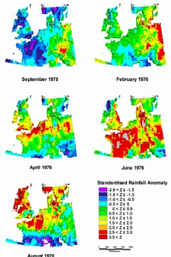
The 1975–76 period was characterised by widespread and severe deficits in both precipitation and streamflow. Figure 1 shows the observed spatial distributions of precipitation anomalies at several key stages within this period. During 1975 and the early part of 1976 there was considerable month-to-month variation in the spatial distribution of ‘drought conditions’. For instance, in the summer of 1975 the British Isles, Denmark and north-western part of France received lower than average rainfall, yet by September 1976 rainfall in these areas was much larger than normal. By spring 1976 the patterns of rainfall anomaly became more persistent, spatially and temporally, with drought across England, northern parts of France and Germany, Denmark and Poland and average or above average rainfall in Mediterranean regions (southern France, Italy and the Balkans). Drought conditions were spatially extensive during June and July 1976, with large areas having anomalies greater than three, with zero precipitation in parts
Fig. 1. Spatial variation in Standardised Monthly Rainfall Anomaly at stages within the 1975/76 drought
of France. After August 1976, precipitation anomalies largely disappeared.
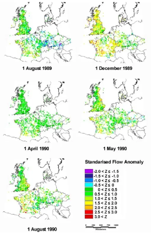
The corresponding flow anomaly distributions are shown in Fig. 2 (flow anomalies maps are given for the 1st day of the following month). Figure 2 suggests that there was a
gradual development of drought conditions over time from summer 1975 onwards. Following the relatively dry summer of 1975 many regions in the UK, France and Germany had moderately high flow anomalies (~1.5) by October 1975. By March 1976, flow deficits were widespread across the
Fig. 2. Spatial variation in Standardised Flow Anomaly at stages within the 1975/76 drought
study area, and anomalies as high as 3 had developed in southern part of the UK and in the Brittany region (France). The situation worsened progressively throughout the summer of 1976 with flow levels eventually returning to normal in the late autumn. Qualitatively, Figs. 1 and 2 suggest a close correlation between the patterns of precipitation deficit/drought and streamflow deficit/drought: in both cases the most severe conditions were observed in southern England, northern France and Germany. Due to a
lack of flow data, it is difficult to assess how the relatively low rainfall received in Mediterranean areas affected streamflow in those regions.
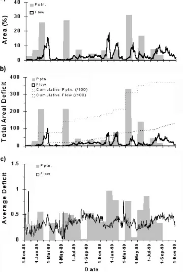
Figure 3 presents the observations discussed above in a quantitative manner, and illustrates the variation in the indices of Drought Area (A), Total Areal Deficit (D) and Cumulative Total Deficit (CTD) for both precipitation and streamflow. In general, there is a good temporal relation between the streamflow and precipitation, with streamflow
drought changing in response to monthly changes in precipitation drought. According to Fig. 3 there is a distinct onset to the drought, in January 1976. This suggests that hydrological conditions in the 1975/76 winter were an important contributing factor in the development of the drought. There is also a distinct end to the streamflow drought in November 1976 (the precipitation drought ended by September 1976). The streamflow drought shows a gradual variation in both area and areal deficit (Figs. 3a and 3b), whereas the precipitation drought is more variable in character. This could be a function of the coarser resolution of the rainfall data, however there is a higher level of auto-correlation in the streamflow time-series than for precipitation, which is the more probable cause.
There are two distinct periods of expansion of streamflow drought, which coincide with expansion of rainfall drought in June and August. The rapid growth during this period corresponds to drought conditions spreading beyond England and France into the rest of Europe as shown by Figs. 1 and 2. There was also a rapid contraction in
streamflow drought at the end of July, along with a period of decreased rainfall deficits. The maximum extent and total deficit of the streamflow drought occurred on 7 July 1976 (about 40% of non-null cells exceeded the drought threshold — equivalent to an area of 200 000 km2). For streamflow,
areal deficit and area follow, broadly, the same pattern of variation as area, and the ratio between the two — the average deficit - is fairly constant over time (Fig. 3c). Furthermore, average streamflow deficit does not respond to changes in average precipitation deficit. This suggests that, in general, changes in streamflow deficit are caused by a large number of cells temporarily crossing the threshold level, rather than an all-round increase in flow anomalies. Increased average streamflow deficit around the end of the drought suggests the occurrence of small areas where high streamflow anomalies persist. These are areas reliant on discharge of groundwater to the river network, and which suffer as a result of reduced groundwater heads.
There is also a strong contrast in cumulative total deficit (CTD) of precipitation and streamflow droughts (note that the cumulative deficit for precipitation has been adjusted to reflect the incremental distribution over each day in the month). The cumulative streamflow deficit is lower than that of precipitation, indicating a high level of damping between precipitation and streamflow systems during the low-flow period (this represents the storage afforded by the soil, groundwater and standing waters).
THE 1989/90 EVENT
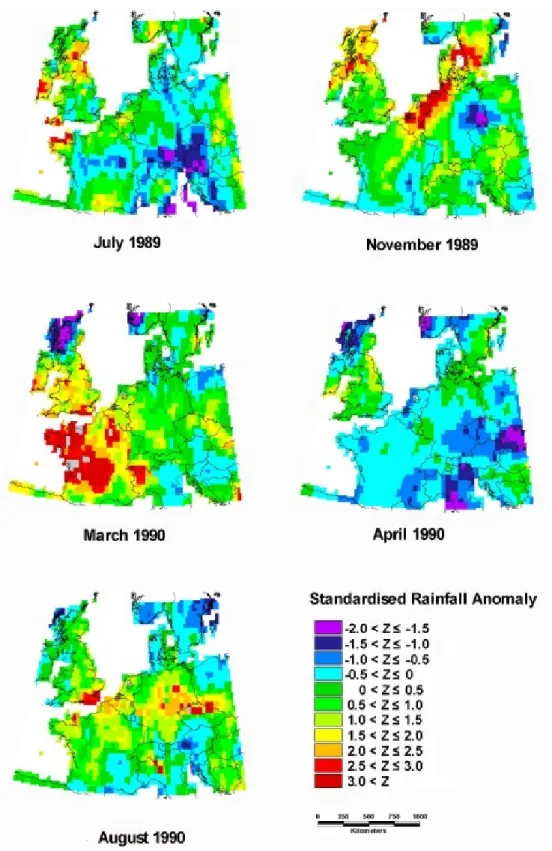
Figures 4 and 5 show some key stages in the evolution of the streamflow and precipitation droughts during the 1989-1990 period. Compared to the 1976 period, precipitation anomalies during 1989/90 are much less coherent in space and time. For example, drought conditions developed on a localised basis, such as in Scandinavia, Netherlands and Scotland during November 1989, in western France and southern England during March 1990, and in eastern Germany in August 1990. Streamflow anomalies, however, were more consistent over time, but there were only a few short-lived and localised streamflow droughts. The worst affected areas include the UK (particularly the north-east) and France.
Figure 6 shows how drought area, total areal deficit and average deficit varied throughout 1989 and 1990 based on a threshold level of 2.0. Whereas the 1975/76 period was characterised by a single distinct drought period from January to September 1976, the 1989/90 period is typified by a high temporal variability in precipitation drought occurrence, which must be related to the atmospheric circulation patterns dominating the area during this period. Fig. 3. Variation in (a) Drought Area (b) Total Areal Deficit and
(c) Average Deficit during the 1975/76 period based on a threshold of 2.0
Fig. 4. Spatial variation in month Standardised Precipitation Anomaly at key points during the 1989/90 period As a result, there seems to be less correlation between the
behaviour of precipitation and streamflow droughts over time. For instance in the summer of 1989 there is a large precipitation drought but negligible streamflow drought (Figs. 6a and 6b), whilst the extent of the streamflow drought
in winter 1989 seems disproportionate to the extent of rainfall drought over the same period (Fig. 6a). There is also a greater disparity between cumulative streamflow and precipitation drought.
Fig. 5. Spatial variation in standardised flow anomaly at key points during the 1989/90 drought
that in the 1976 event, roughly 0.5, but is highly variable over time. Figure 6c suggests that 1989/90 can be split into three broad periods, each exhibiting different drought behaviour. Firstly, a period in which drought is localised but relatively severe is observed between June and November 1989 (drought area is small, but average deficit is fairly large). In the second period, over winter 1989/90,
there are several episodes in which the flow anomalies in large areas of Europe exceeded the drought threshold for a short time (the largest deficit area was recorded during December 1989 and equalled 70 000km2). Finally, a more
extensive and persistent drought took place between June and October 1990.
INFLUENCE OF PRECIPITATION ON STREAMFLOW DROUGHT
The observations shown in Figs. 1 to 6 suggest that the relationship of streamflow drought to precipitation drought is both lagged and damped, as would be expected, due to catchment storage. These aspects were investigated further, for the 1975/76 event, by determining the level of correlation between different streamflow and precipitation drought indices. The streamflow drought indices were therefore re-evaluated at a monthly time step, so that they could be compared more readily with the precipitation data.
The correlations between monthly streamflow drought area, Af (m), and precipitation drought area, Ap,for various
lag intervals and durations are reported in Table 1a. Similarly, Table 1b details the correlation between the total area deficits Df(m) and Dp(m). In this case the sample set was also partitioned into two sub-sets, one for those months where streamflow drought deficits were high (Df > 10) and one for those months having low values (Df < 10)
In this case the sample set was also partitioned into two sub-sets months, one containing high values of streamflow drought deficit (Df > 10) and one containing low values (Df<10). Table 1c details the correlation coefficient when cumulative deficits (from January 1976 to month m Fig. 6. Variation in (a) Drought Area (b) Total Areal Deficit and
(c) Average Deficit during the 1989/90 period based on a threshold of 2.0.
Table 1a. Correlation Coefficients (Pearson) between
monthly drought area based on streamflow (Af) and precipitation (Ap)data. Af (m) Ap (m) 0.59 Ap (m-1) 0.57 Ap (m-2) 0.41 (m,m 1) p
A
− 0.87 (m,..,m 2) pA
− 0.94 (m,..,m 3) pA
− 0.94 (m,..,m 4) pA
− 0.82Table 1b. Correlation Coefficients (Pearson) between
monthly areal deficit based on streamflow (Df) and precipitation (Dp) data. Df (m) All months Df < 10 Df > 10 Dp (m) 0.55 0.47 0.08 Dp (m-1) 0.60 Dp (m-2) 0.33 (m,m 1) p
D
− 0.87 0.83 -0.13 (m,..,m 2) pD
− 0.95 0.91 -0.06 (m,..,m 3) pD
− 0.78 0.88 -0.06 (m,..,m 4) pD
− 0.60 0.38Table 1c. Correlation Coefficients (Pearson) between
monthly cumulative total deficit based on streamflow (CTDf) and precipitation (CTDp) data.
CTDf (m) 3–Month 9-Month Running Running Average CTDf Average CTDf (m) (m) CTDp (m) 0.96 3-Month RA CTDp (m) 0.91 9-Month RA CTDp(m) 0.98
inclusive) are considered. In each case the Pearson Correlation Coefficient is shown. Pearson correlations vary between –1 and +1. A value of 0 indicates that neither of the two variables can be predicted from the other by using a linear equation, whereas a value of 1 or –1 indicates that one variable can be predicted perfectly by a linear function of the other.
Tables 1a and 1b indicate that, whilst the areas are moderately correlated linearly at small lags, there is a better correspondence between streamflow drought area at month m and the average precipitation drought area over the previous two to four months. A similar result is obtained when areal deficits are compared. Furthermore there is an extremely strong agreement between the cumulative deficits for streamflow and precipitation where the cumulative period is from January 1976 to month m, and where the 3-month and 9-3-month running average deficits are considered.
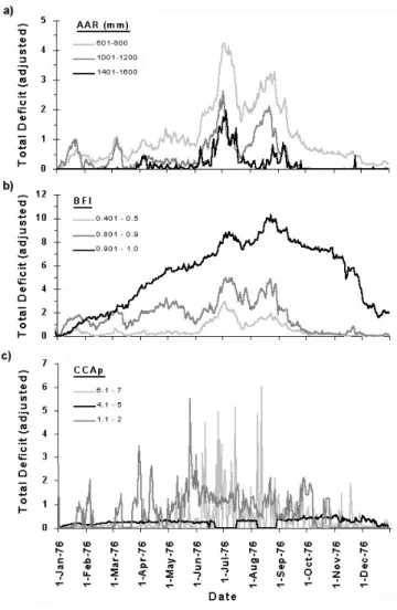
The influence of catchment properties, such as climate and permeability, on streamflow drought were also considered. Using average annual rainfall as an indicator of climate, and Baseflow Index (Institute of Hydrology, 1980) as an indicator of catchment permeability, cells were grouped according to the property of interest and, at each time step, Df values were recalculated for each group. The results are illustrated in Fig. 7 — in each case the total deficit is adjusted according to the proportion of non-null cells in the group for each group (note that, for clarity, only curves for selected groups are shown). In Figure 7a, cell grouping was based on the average annual rainfall (1960-95) value for each cell derived from the CRU data set, whilst in Fig. 7b the grouping is by Baseflow Index of the cell (derived from flow data). For comparison, a further grouping is made according to the cumulative cell precipitation anomaly CCAp (i.e. sum of the anomaly values recorded at a cell over a period of time) from 1st January to 1st September 1976 (Fig. 7c). The CCAp is intended to reflect the typical size of Pi at each cell, i, during the lifetime of the drought event.
When compared to the variability of Df over time for the study area as a whole (Fig. 3b), Fig. 8a indicates the climate
Fig. 7. Variation in Total Area Deficit (streamflow) grouped
according to (a) average annual rainfall for 1960-95 period and (b) Base Flow Index (BFI) (c) CCAp for the period from
1 January 1976 to 1 September 1976
Fig. 8. Relationship between cell precipitation anomalies and cell
has little influence on the temporal variation of drought deficit, although areas with ‘wetter’ climates tended to have lower streamflow deficits. Figure 7b suggests that Baseflow Index has a strong influence on the variation of streamflow drought deficit over time. The group containing cells with large baseflow values (i.e. the most permeable areas within the study area) shows a distinct pattern of variation over time, which is very different to that for the study area as a whole. Within this group there is a reduced day-to day variation in Df, for instance the June and August peaks are much less dominant, and the deficit is larger in magnitude than that of other zones. Figure 7c shows a less clear distinction between groups, but where CCAp is high there are many short-lived drought events, whereas where CCAp is low there is less variability over time.
INFLUENCE OF CELL PRECIPITATION ANOMALY ON CELL STREAMFLOW ANOMALY
The following results explore the relation between streamflow and precipitation anomalies at cell level (i.e. whether a particular grid cell has similarly sized streamflow deficit and precipitation deficit at a particular moment in time).
Tables 2a, b and c give details of the correlation coefficients between the cell streamflow anomaly index Fi, and deficit Di (f) and the corresponding values derived from
the precipitation data. The results are presented for four particular days during the drought period, the 1st March, 1st May, 1st July and 1st September. Whilst Table 2a indicates a moderate relationship between flow and precipitation anomalies, Table 2b demonstrates that there is a poor relationship when the drought status is considered with Di(f) and Di(p) having a negligible relationship, even when average conditions over the last two months are considered. This suggests that, whilst precipitation anomalies have a fairly large control over the size of the flow anomaly at a particular point in time, the most severe streamflow anomalies were not occurring in the catchments with the most severe precipitation anomalies.
There is also some variation depending on the day considered, for example streamflow anomalies on 1st March
show a high level of correlation with the values of precipitation anomaly for the corresponding cells, whilst those on 1st September do not, as illustrated in Fig. 8. This
demonstrates that antecedent storage conditions affect the degree to which precipitation conditions affect the amount of flow depletion.
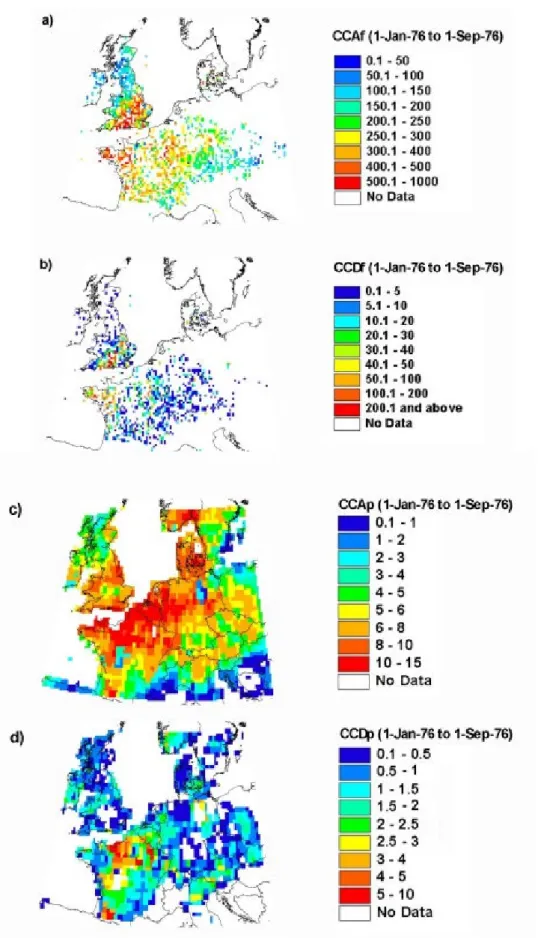
Figure 9 shows the spatial distribution of the cumulative anomaly (counting time steps where the anomaly score is greater than 0) and drought deficits (counting all time steps
where the anomaly score is greater than 2) at each cell between 1st January and 1st September. Maps for both streamflow (Figs. 9a and b) and precipitation (Figs. 9c and d) are shown. In each case, there is a broadly similar pattern of cumulative anomaly and deficit (i.e. in general, areas with relatively high cumulative precipitation deficit also experienced relatively high streamflow deficits).
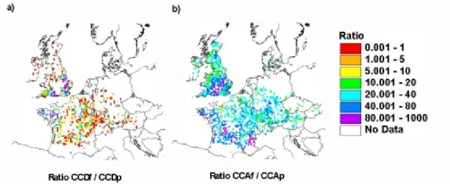
Figure 10 shows the resulting spatial distributions when the ratios of corresponding pairs are determined. Note that ratios have not been adjusted to account for the differing resolution of the streamflow and precipitation data sets. Therefore, a ratio of around 20, roughly represents equivalent streamflow and precipitation depletion. In regions where the ratio is smaller than 20, the cumulative precipitation deficit is large relative to the streamflow deficit (i.e. there is a large degree of damping in the system), but where the ratio is larger than 20, the streamflow depletion
Table 2a. Relation between cell streamflow and precipitation
anomaly scores
Fi on day d
d = 1st Mar d = 1st May d = 1st July d = 1 Sept
Pi(m-1) –0.43 0.40 0.29 0.21 Pi (m-2) 0.47 –0.07 0.42 0.23
(m 1,m 2)
i
P
− − 0.54 0.24 0.41 0.26 Table 2b. Relation between cell streamflow and precipitationdeficits
Di (f) on day d
1st Mar 1st May 1 Sept
Di (p) (m-1) –0.06 0.11 –0.09
Di (p) (m-2) 0.03 –0.08 –0.02
(m 1,m 2)
i
D
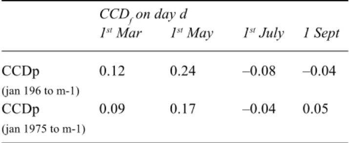
− − 0.01 0.01 –0.08Table 2c. Relation between cell cumulative deficit for
streamflow and precipitation drought
CCDf on day d
1st Mar 1st May 1st July 1 Sept
CCDp 0.12 0.24 –0.08 –0.04
(jan 196 to m-1)
CCDp 0.09 0.17 –0.04 0.05
Fig. 9. Spatial distribution of (a) Cumulative Cell Anomaly and (b) Cumulative Cell Deficit for the period from 1st January 1976 to
1st September 1976 based on streamflow data and (c) Cumulative Cell Anomaly and (d) Cumulative Cell Deficit for the period from
is large relative to the precipitation depletion. The correlation coefficient between the two maps is 0.49 indicating a general relationship between the two. However, the maps shown in Fig. 10 suggest that southern England and northern France have a behaviour distinct from the rest of the study area. Within this zone, streamflow anomalies and deficits are much higher than the corresponding precipitation anomalies and deficits. Elsewhere in Europe, there is a one-to-one relationship between flow anomaly and precipitation anomaly, whilst streamflow deficits are generally lower than precipitation deficits. These findings suggest that in southern England and northern France some additional factor reduces the amount of damping between precipitation and streamflow anomalies, and that the level to which this occurs is related to the size of the anomaly.
Three possible factors that may explain this discrepancy were considered: climate, groundwater discharge and the cumulative amount (over time) of precipitation depletion. The relationships between the cell drought status of these variables(Fi, Di (f) and CCD(f)) were considered. As before, the grid cells were grouped according to average annual rainfall, Baseflow Index and cumulative cell anomaly up to 1st September, and the mean value of each index calculated on a group-wise basis (Tables 3a, b and c). The mean cell value for each zone is given in each case. In general, regions with low average annual rainfall had higher anomaly values of the drought indices than those in wetter climates. However, when only those cells with anomaly index values of 2 or more were considered, the behaviour was more uncertain. Regions with high baseflow values had higher flow anomalies and cumulative anomalies than catchments with low rainfall (Table 3a). This observation also held true when the more severely affected cells were considered (i.e.
mean drought deficit and cumulative deficit also increased with increasing baseflow). Interestingly, there was no clear pattern between the streamflow anomaly or drought magnitude and the cumulative rainfall anomaly (Table 3c). It is evident that the degree of storage, as represented by BFI, influences the correlation between cell streamflow and precipitation anomaly. This can be shown easily by examining how the values of the correlation coefficient between corresponding flow anomaly and precipitation anomaly change when cells of different Baseflow Index (BFI) are considered. For example, on the 1st July 1976, the correlation coefficient between Fi and Pi (average of last two months) was 0.68 for catchments with BFI of 0.4 or less, 0.45 for catchments with BFI in the range 0.4 to 0.7 and 0.03 for catchments with BFI greater than 0.7.
Figure 11 illustrates how anomaly values within a particular grid cell vary in relation to one another. The time series for two contrasting cells are shown. In (a) the cell has an average Base Flow Index of 0.45 whilst the Base Flow Index of (b) is 0.9. For cell (a) there is a large day to day variation in streamflow anomaly over time, and the magnitude of the anomaly agrees closely with that of precipitation. At cell (b) the streamflow anomaly shows less dependence on precipitation anomaly. Streamflow depletion continues to rise even where precipitation anomaly becomes negative, and a high flow anomaly is maintained for some time at the end of the drought period even when there has been above average precipitation for several months. The different characteristics of the two stations reflect the fact that runoff in cell (a) is directly proportional to rainfall, whilst in cell (b) streamflow depletion is controlled by the amount of baseflow depletion. A plentiful supply of groundwater discharge may sustain streamflow levels Fig. 10. Spatial distribution of ratios between (a) Cumulative Cell Deficits for streamflow and precipitation and and
Table 3a. Variation of cell characteristics with Average Annual Precipitation (values given are mean value per group)
Range of Average Annual Precipitation (mm) represented in group
up to 601– 801– 1001– 1201– 1401– 1601– 1801– above
600 800 1000 1200 1400 1600 1800 2000 2001
CCAf (1-Jan to 1-Sep) 1.18 1.24 1.10 0.97 0.77 0.73 0.76 0.55 0.60
Fi (1 May 1976) 1.30 1.40 1.12 1.05 0.94 0.99 1.22 0.98 0.79
Fi (1 September 1976) 1.87 1.72 1.45 1.37 1.33 1.21 1.20 1.34 1.54
CCDf (1-Jan to 1-Sep) 0.08 0.11 0.07 0.06 0.02 0.02 0.04 0.01 0.02
Di (f) (1 May 1976) 0.26 0.56 0.50 0.25 0.07 0.29 2.27 N/A N/A
Di (f) (1 September 1976) 0.71 0.61 0.43 0.58 0.28 0.50 0.31 0.28 0.56
Table 3b. Variation of cell characteristics with Baseflow Index Precipitation (values given are mean value per group) Range of BFI values represented in group
up to 0.21– 0.31– 0.41– 0.51– 0.61– 0.71– 0.81– 0.91–
0.2 0.3 0.4 0.6 0.6 0.7 0.8 0.9 1.0
CCAf (1-Jan to 1-Sep) 0.77 0.00 0.85 1.04 1.08 1.12 1.14 1.37 1.63
Fi (1 May 1976) 0.93 N/A 0.99 1.18 1.20 1.20 1.21 1.58 1.90
Fi (1 September 1976) 1.32 N/A 1.40 1.52 1.56 1.47 1.52 1.77 2.36
CCDf (1-Jan to 1-Sep) 0.05 0.00 0.05 0.06 0.07 0.07 0.08 0.19 0.41
Di (f) (1 May 1976) N/A N/A 0.23 0.38 0.48 0.34 0.39 0.92 1.03
Di (f) (1 September 1976) N/A N/A 0.43 0.47 0.50 0.46 0.59 0.66 1.00
Table 3c. Variation of cell characteristics with Cumulative Rainfall Anomaly Precipitation (values given are mean value per
group)
Range of CCAp values represent in group
up to 1 1.01-2 2.01-3 3.01-4 4.01-5 5.01-6 6.01-8 8.01-10 10 &
above
CCAf (1-Jan to 1-Sep) 0.96 1.05 0.94 0.77 0.83 0.99 1.15 1.24 1.20
Zi (f) (1 May 1976) –0.22 0.97 0.97 0.60 0.92 1.07 1.30 1.47 1.38
Zi (f) (1 September 1976) 1.26 1.21 1.19 1.00 1.24 1.38 1.63 1.77 1.74
CCDf (1-Jan to 1-Sep) N/A 0.03 0.04 0.02 0.05 0.08 0.10 0.10 0.06
Di (f) (1 May 1976) N/A N/A 1.28 N/A 0.39 0.68 0.59 0.44 0.33
Di (f) (1 September 1976) N/A 0.45 0.32 0.27 0.43 0.40 0.56 0.57 0.44
through a drought. However, when this source is exhausted, streamflows will be highly anomalous, regardless of the availability of rainfall, as shown by the behaviour of catchment (b).
Discussion
The study shows that the spatial distribution of rainfall anomalies strongly determines where droughts will occur. However, the difference in character between the 1975/76
Table 4. Relation between streamflow anomalies and
precipitation anomalies at two cells
Fi (m) Cell A Fi (m) Cell B Pi (m) 0.22 -0.17 Pi (m-1) 0.31 0.68 (m,m1) i P − 0.38 0.31 Pi (m-2) 0.48 0.11 (m1,m 2) i P − − 0.58 0.57
and 1989/90 droughts illustrates the importance of the timing and duration of periods with reduced rainfall. The temporal persistence of rainfall deficiencies strongly influences the severity of the drought event as a whole. As rainfall deficiencies were both greater and more persistent during 1976, the 1976 drought was, in terms of streamflow drought, much larger (maximum gauged extent of 200 000 km2 as
opposed to 50 000 km2) and more severe (cumulative total
deficit of 250 compared to 100) than the 1989/90 event. The 1976 drought was also more coherent, having a well-defined start and end. In contrast, the 1989/90 period was characterised by a series of short drought events, with much greater variability over time. The rapid changes in drought occurrence during 1989/90 were caused by short-term variations in the synoptic weather situation over Europe.
The analysis indicated that streamflow responds in a delayed and damped manner to the occurrence of precipitation deficits. For the 1975/76 event, streamflow drought magnitude was correlated to the average precipitation deficit over the preceeding two to four months. When the cumulative precipitation and streamflow deficiencies at the end of the drought period were considered there was a high correlation between the spatial distribution
of values. For the drought as a whole, the level of damping increased as the anomaly levels increased and, at the height of the drought period, the extent and deficit of streamflow drought was much smaller than that of precipitation.
In both droughts streamflow deficiencies tended to be most severe in the southern UK and in northern France. Recent work has suggested that weather patterns associated with the North Atlantic Oscillation influence the spatial distribution of drought severity in Europe (Shorthouse and Arnell, 1997; Stahl and Demuth, 1999). However, given the wide variety of hydrological regimes across Europe, it is difficult to accept that catchment characteristics do not play a strong role in drought development. This theory is supported by the facts that the areal pattern of streamflow drought in the worst affected regions (e.g. see 1st May on Fig. 2) is very different from the distribution of rainfall drought over the same area, and that the most severe streamflow anomalies did not occur in the grid cells with the most severe precipitation anomalies. Furthermore, the results shown in Fig. 10 suggest that drought conditions in southern England and northern France were much worse that would be expected given the level of precipitation deficiency in those regions.
The analyses indicated that catchment geology plays a predominant role in moderating or accentuating the amount of streamflow drought. In permeable areas, there was a weaker relation between streamflow and precipitation anomalies, both in space (as shown by the cell to cell correlation tests) and in time (as shown by the difference in drought deficit for groups of cells with different BFI values). Conversely climate had little influence on the temporal drought development, although areas with ‘wetter’ climates tended to have lower streamflow deficits. At the height of the drought, regions with high baseflow values had higher flow anomalies. At first this seems a contradiction in terms. Groundwater discharge usually supports flow levels during the low flow period, affording a smaller day to day dependence on precipitation. However, if the drought is long or extends over the autumn recharge period, reduced levels of groundwater recharge may result in a gradual decline in the piezometric surface and a decline in groundwater discharge. In this situation, extremely high flow anomalies would be assigned to the stream. This theory fits the behaviour of the 1975/1976 drought, in which there was a sustained period of low rainfall from summer 1975 and over the 1975/1976 winter. Furthermore, the severest drought occurred in southern UK and northern France, a region that is dominated by aquifer systems such as the Chalk.
This study has highlighted the need for improved understanding of the links between meteorological droughts Fig. 11. Illustration of the role played by catchment permeability:
variation of anomaly over time for grid cell (a) having low BFI and (b) having high BFI
and streamflow droughts but would also have benefited from a greater availability of flow data within the study area. Further work might examine a larger number of drought events, or examine the role of scale effects on quantification of drought characteristics.
Conclusions
In terms of streamflow depletion, the 1976 drought was a highly coherent event, having a well defined start (in January 1976) and end (in September 1976). The worst and most persistent streamflow droughts occurred in southern England and northern France. Central parts of Europe experienced severe streamflow depletion only during the ‘height’ of the drought in June, July and August when there was negligible precipitation across large areas of Europe. In contrast, the 1989/90 period was characterised by a series of shorter and less severe droughts, with much greater variability over time. There was, also, a less clear relationship between precipitation drought and streamflow drought; this might have resulted from periods of precipitation depletion occurring randomly in time. Particularly high levels of streamflow drought were again suffered in southern England and northern France.
Several possible explanations for the increased drought over southern England and northern France were investigated using data from the 1976 event. However, immediate precipitation deficits could not explain the level of streamflow depletion in these areas. Rather, the level of streamflow depletion was enhanced by decreased discharge of groundwater into the river networks in this region; this can be attributed to large precipitation deficits during autumn 1975 and spring 1976 which reduced the winter groundwater recharge, leading ultimately to depressed groundwater levels.
Early prediction of drought events relies upon identification of streamflow deficiencies, and assessment of the likelihood that they will remain, or get worse. Coupled with a dense network and database of gauging stations monitored in near real time, the improved understanding of past drought events gained from this study might eventually be used operationally to predict and mitigate future droughts in Europe.
Acknowledgements
The authors would like to acknowledge the use of streamflow data from the FRIEND (Flow Regimes from International Experimental and Network Data) European
Water Archive. Part of the research presented in this paper was carried out within the framework of the ARIDE Project (Assessment of the Regional Impact of Droughts in Europe), supported by the European Commission under Contract no. ENV4-CT97-05533.
References
Acreman, M.C. and Adams, B., 1998. Low flow, groundwater and
wetland interactions. Report to Environment Agency (W6-013),
UKWIR (98/WR/09/1) and NERC (BGS WD/98/11) Institute of Hydrology, Wallingford, UK.
Beran, M. and Rodier, J.A., 1985. Hydrological aspects of drought. Studies and reports in hydrology, 39, UNESCO-WMO, Paris, France.
Bordi, I. and Sutera, A., 2001. Fifty years of precipitation: some spatially remote teleconnections. Water Res. Manage., 15, 247– 280.
Bradford, D., 2000. Drought Events in Europe. In: Drought and
Drought Mitigation in Europe, J.V. Vogt and F. Somma, (Eds.).
Kluwer, Dordrecht, The Netherlands. 7–22.
Briffa, K.R., Hones, P.D. and Hulme, M., 1994. Summer moisture variability across Europe,1892-1991. An analysis based on the Palmer Drought Severity Index. Int. J. Climatol., 14, 475–506. Dracup, J.A., Seong Lee, K, and Paulson, E.G., 1980. On the
Definition of Droughts. Water Resour. Res., 16, 297–302. Garriodo, A. and Gomez-Ramos, A., 2000. Socio-economic
Aspects of Droughts. In: Drought and Drought Mitigation in
Europe, J.V. Vogt and F. Somma, (Eds.). Kluwer, Dordrecht,
The Netherlands. 197–207.
Grindley, J., 1979. Rainfall. In: Atlas of Drought in Britain,
1975-1976, J.C. Doornkamp and K.J. Gregory, (Eds.). Institute of
British Geographers. 28–29.
Hisdal, H., Tallaksen, L.M., Peters, E., Stahl, K. and Zaidman, M., 2001. Drought Event Definition. In: Assessment of the
Regional Impact of Droughts in Europe, S. Demuth and K. Stahl
(Eds.). Final Report to the European Union ENV-CT97-0553, Institute of Hydrology, University of Freiburg, Germany. 17– 26.
Institute of Hydrology Report, 1980. Low Flow Studies Report. Institute of Hydrology, Wallingford, UK.
Krasovskaia, I. and Gottschalk, L., 1995. Analysis of regional drought characteristics with empirical orthogonal functions. In:
New uncertainty concepts in hydrology and water resources,
Z.W. Kundezewicz, (Ed.). International Hydrology Series, Cambridge University Press, Cambridge, UK. 163–167. McKee, T.B., Doesken, N.J. and Kleist, J., 1993. The Relationship
of Drought Frequency and Duration to Time Scales. Proceedings
of the 8th Conference on Applied Climatology, Boston, USA.
American Meteorological Society.
New, M.G., Hulme, M. and Jones, P.D., 2000. Representing twentieth-century space-time climate variability. Part II: Development of 1901-1996 monthly grids of terrestrial surface climate. J. Climate, 13, 2217–2238.
Palmer, W.C., 1965. Meteorological drought. Weather Bureau Research Paper No 45. US Dept of Commerce, Washington D.C., USA.
Rees, H.G. and Demuth, S., 2000. The application of modern information system technology in the European FRIEND project. Wasser and Boden, 52, 9–13.
Santos, M.A., 1983. Regional droughts; a stochastic characterisation. J. Hydrol., 66, 183–211.
Santos, M.J., Verissimo, R. and Rodrigues, R., 2001. Drought Distribution Model. In: Assessment of the Regional Impact of
Droughts in Europe, S. Demuth and K. Stahl (Eds.). Final Report
to the European Union ENV-CT97-0553, Institute of Hydrology, University of Freiburg, Germany, 69–79.
Sen, Z., 1998. Probabalistic formulation of spatio-temporal drought pattern. Theor. Appl. Climatol., 61, 197–206.
Shorthouse, C.A. and Arnell, N.W., 1997. Spatial and temporal variability in European river flows and the North Atlantic oscillation. In: FRIEND-97- Regional Hydrology: Concepts and
Models for Sustainable Water Resource Management
(Proceedings of the conference held in Postonjna, Slovenia, September 1997. IAHS Publ. no 246. 77–85.
Smithson, P.A., 1980. Rainfall. In: Atlas of Drought in Britain,
1975-1976, J.C. Doornkamp and K.J. Gregory (Eds.). Institute
of British Geographers. 16–17.
Stahl, K. and Demuth, S., 1999. Linking streamflow drought to the occurrence of atmospheric circulation patterns. Hydrol. Sci.
J., 44, 467–482.
Subrahmanyan, V.P., 1967. Incidence and Spread of Continental
Drought. WMO/IHD Project Report No 2. Secretariat of the
World Meteorological Organisation, Geneva, Switzerland. Szinell, C.S., Bussay, A. and Szentimrey, T. ,1998. Drought
tendencies in Hungary. Int. J. Climatol., 18, 1479–1491. Tallaksen, L.M., 2000. Streamflow drought frequency analysis.
In: Drought and Drought Mitigation in Europe, J.V. Vogt and F. Somma (Eds.). Kluwer, Dordrechet, The Netherlands. 103– 117.
Tase, N., 1976. Area-deficit-intensity characteristics of droughts. Hydrology Paper 87. Colorado State University, Fort Collins, USA.
Wilhite, D.A., 1993. Drought assessment, management, and
planning : theory and case studies. Kluwer, Boston, USA.
Yevjevich, V., 1967. An Objective Approach to Definition and
Investigations of Continental Hydrologic Droughts. Hydrology