Publisher’s version / Version de l'éditeur:
Vous avez des questions? Nous pouvons vous aider. Pour communiquer directement avec un auteur, consultez la
première page de la revue dans laquelle son article a été publié afin de trouver ses coordonnées. Si vous n’arrivez pas à les repérer, communiquez avec nous à [email protected].
Questions? Contact the NRC Publications Archive team at
[email protected]. If you wish to email the authors directly, please see the first page of the publication for their contact information.
https://publications-cnrc.canada.ca/fra/droits
L’accès à ce site Web et l’utilisation de son contenu sont assujettis aux conditions présentées dans le site LISEZ CES CONDITIONS ATTENTIVEMENT AVANT D’UTILISER CE SITE WEB.
Proceedings of the World Congress on Evolutionary Computation, 2003
READ THESE TERMS AND CONDITIONS CAREFULLY BEFORE USING THIS WEBSITE.
https://nrc-publications.canada.ca/eng/copyright
NRC Publications Archive Record / Notice des Archives des publications du CNRC :
https://nrc-publications.canada.ca/eng/view/object/?id=2639f4b1-63ad-4f00-92d7-0d7a03d74930
https://publications-cnrc.canada.ca/fra/voir/objet/?id=2639f4b1-63ad-4f00-92d7-0d7a03d74930
NRC Publications Archive
Archives des publications du CNRC
This publication could be one of several versions: author’s original, accepted manuscript or the publisher’s version. / La version de cette publication peut être l’une des suivantes : la version prépublication de l’auteur, la version acceptée du manuscrit ou la version de l’éditeur.
Access and use of this website and the material on it are subject to the Terms and Conditions set forth at
An Evolution Strategies Approach to the Simultaneous Discretization of
Numeric Attributes in Data Mining
National Research Council Canada Institute for Information Technology Conseil national de recherches Canada Institut de technologie de l'information
An Evolution Strategies Approach to the
Simultaneous Discretization of Numeric Attributes
in Data Mining *
Valdés, J., Molina, L.C., and Peris, N.
December 2003
* published in Proceedings of the World Congress on Evolutionary Computation.
Canberra, Australia. December 8-12, 2003. IEEE Press 03TH8674C, ISBN 0-7803-7804-0, pp. 1957-1964. NRC 46536.
Copyright 2003 by
National Research Council of Canada
Permission is granted to quote short excerpts and to reproduce figures and tables from this report, provided that the source of such material is fully acknowledged.
An Evolution Strategies Approach to the Simultaneous Discretization of
Numeric Attributes in Data Mining
Julio J. Vald´es
National Research Council of Canada Institute for Information Technology
M50, 1200 Montreal Rd. Ottawa, ON K1A 0R6, Canada
Luis Carlos Molina
Mexican Institute of Petroleum L´azaro C´ardenas 152
07720, Mexico City Mexico [email protected]
Nat´an Peris
CSA Integraci´on de Sistemas Mare de Deu de les Neus 72
08031, Barcelona, Spain [email protected]
Abstract- Many data mining and machine learning algo-rithms require databases in which objects are described by discrete attributes. However, it is very common that the attributes are in the ratio or interval scales. In order to apply these algorithms, the original attributes must be transformed into the nominal or ordinal scale via dis-cretization. An appropriate transformation is crucial because of the large influence on the results obtained from data mining procedures. This paper presents a hybrid technique for the simultaneous supervised dis-cretization of continuous attributes, based on Evolution-ary Algorithms, in particular, Evolution Strategies (ES), which is combined with Rough Set Theory and Informa-tion Theory. The purpose is to construct a discretizaInforma-tion scheme for all continuous attributes simultaneously (i.e. global) in such a way that class predictability is maxi-mized w.r.t the discrete classes generated for the predic-tor variables. The ES approach is applied to 17 public data sets and the results are compared with classical dis-cretization methods. ES-based disdis-cretization not only outperforms these methods, but leads to much simpler data models and is able to discover irrelevant attributes. These features are not present in classical discretization techniques.
1 Introduction
Many data mining and machine learning algorithms [Qui89] [CN89] [FKY96] require data in which objects are de-scribed by sets of discrete attributes. In practice, however, a great number of attributes are of a continuous nature, as they come from measurements, sensors, etc. (e.g. temper-ature, weight). Therefore in order to use these algorithms, the continuous attributes must be transformed into discrete, but the way in which it is done have a large impact on the results obtained by the data mining techniques.
Several techniques have been proposed for both the su-pervised and unsusu-pervised case [And73] [Ker92] [FI93], [MRMC00]. In the former one, the class information of the studied objects is available and can be used for guiding the discretization process. Algorithms like k-means, ChiMerge and partition using Minimal Description Length Principle (MDLP) [FI93] belong to this family and are popular. How-ever, they were formulated for transforming only one con-tinuous attribute at a time. Further, the number of classes or intervals for partitioning the attribute must be set forth in
ad-vance (e.g. k-means), and in others, some significance level must be established (e.g. ChiMerge). Usually these parame-ters are given by the expert or found using other techniques. In the multivariate case these techniques perform the dis-cretization in an attribute-wise manner. That is, each vari-able is transformed separately. However, with this approach the inter-relations within the prediction attributes is not tak-ing into account. In real world data, attributes are usually interrelated in subtle, non-linear ways, and redundancies of different degrees are present. Therefore, the discretiza-tion of each attribute independently of the others may lead to important information losses, thus increasing the chance of missing interesting relations in the knowledge discovery process.
This paper presents a hybrid technique for the simultane-ous supervised discretization of continusimultane-ous attributes, based on evolutionary algorithms (in particular, Evolution Strate-gies (ES) [Rec73] [Bac91]). It also uses Rough Set Theory [Paw82] [Paw91] and Information Theory, as is done in in-ductive learning [Qui86] [Qui96]. The purpose is to gen-erate a global discretization scheme for all continuous at-tributes simultaneously by exploiting the inter-attribute rela-tions, in addition to the dependency between the class vari-able and each attribute. Class predictability is maximized w.r.t a given criterium by relating the discrete classes con-structed for the predictor attributes with the classes of the decision attribute. A discretization of a continuous attribute is given by a crisp partition of its range by a set of real val-ues (cut points). The cardinality of this set determines the number of classes into which the given attribute is to be par-titioned, and the cut-points, the intervals defining each class. A joint (global) discretization scheme for a set of attributes is given by the number of classes in which each particu-lar attribute is partitioned, and the set of cut points defining them.
The paper is organized as follows: Section 2 presents the discretization problem. Section 3 approaches discretization from an evolutionary algorithms perspective (focussing on evolution strategies), and presents algorithms based on three criteria. Section 4 presents three different experiments per-formed with different data sets and Section 5 discusses the results obtained, as well as comparisons with two classical discretization methods. The conclusions are presented in Section 6.
2 The Simultaneous Discretization of Numeric
Attributes
Consider an information system S =< U, A > [Paw82] where U and A are non-empty finite sets, called the universe and the set of attributes respectively, such that each a ∈ A has a domain Va and an evaluation function fa assigns to
each u ∈ U an element fa(u)∈ Va(i.e. fa(u) : U → Va).
Typical examples of are data matrices with nominal or ordi-nal attributes. Sometimes, A is of the form ApS{d}, where
the set Ap is called prediction attributes and d the decision
attribute. A more general kind of information system is ob-tained if the elements of A have domains given by arbitrary sets, not necessarily finite (for example, if Va ⊆ R, where
R is the set of real numbers). Data matrices with inter-val or ratio variables are examples of systems of this kind. Consider two information systems Sd =< U, Ad >and
Sc =< U, Ac >with the same universe U and attributes
A, but with different domains. Thus, the attributes have the same cardinality n = card(Ad) = card(Ac), and the
information systems are defined as: for all ad
∈ Ad and
u ∈ U, fad(u) : U → Vadd ⊂ N+ (N+ is the set of
nat-ural numbers and Vd
ad is finite). Sc =< U, Ac >and for
all ac ∈ A
cand u ∈ U, fac(u) : U → Vacc ⊆ R (R is the
set of real numbers). A discretization between information systems is a mapping D : Sc→ Sd.
Discretizations can be defined in many ways. Here a Discretization is considered to be given by a collection of parametrized functions ϕi, 1 ≤ i ≤ n of the form:
Vd
ai = ϕi(V
c ai, . . . , V
c
ai, ˆpi), where ˆpiis a set of parameters.
These functions map the sets of domains of the attributes in Ac to those in Ad and leads to a global discretization,
in the sense that the transformation of a particular attribute depends on all of them. In the particular case in which Vd
ai = ϕi(V
c
ai, ˆpi)the discretization is attribute-wise or
lo-cal. Global or local discretizations can be easily constructed if a collection of natural numbers M = {m1, . . . , mn}
(mi ∈ N+, 1 ≤ i ≤ n), and a collection of vectors
T = {~t1, . . . , ~tn} are given s.t. ~ti ∈ Rmifor all 1 ≤ i ≤ n.
For a given attribute ai, the corresponding vector ~tiinduces
a partition of Vc
aiinto mi+ 1adjacent classes or categories.
The elements of ~tiare called cut-points.
Examples of popular supervised discretization meth-ods are the ChiMerge [Ker92] and the one introduced in [FI93], using the the Minimum Description Length Prin-ciple (MDLP) [Ris86]. The ChiMerge method is a statis-tically based approach for attribute-wise discretization. At the beginning it places each numeric value into its own class and merge them according to a χ2 test applied to
neigh-boring classes. The hypothesis tested is that two adjacent classes are independent, which is based on the comparison between the expected and observed frequencies of values found in the corresponding classes. The merging procedure is applied until a χ2-threshold is reached.
The MDLP was applied to the discretization problem in [FI93] within a recursive entropy minimization heuristic for controlling the generation of decision trees. A coding scheme is defined which enables the comparison of
infor-mation gains obtained with different cut points of the stud-ied attribute, in terms of their codifstud-ied lengths. Then, they are accepted or rejected according to the MDLP criterium. These two methods will be used for compararing the ES-based discretizations introduced in the next section.
3 An Evolutionary Algorithm Approach to
Su-pervised Simultaneous Discretization
The power of evolutionary algorithms (EA) in solving func-tion optimizafunc-tion problems makes genetic algorithms, evo-lution strategies, and others, a natural choice from a compu-tational intelligence perspective to the discretization prob-lem. An evolutionary computation-based discretization al-gorithm can be expressed as D =< EA, Cr,Par, P >
where EA is an evolutionary algorithm, Cr is a criterium
for evaluating the quality of the mapping, Par a collection of parameters controlling the algorithm, and P is a post-processing stage. The post-post-processing stage used here con-sist on removing cut-points without affecting the value of the fitness function. It leads to important model simplifica-tions.
3.1 An Evolution Strategy Approach to Simultaneous Discretization
Evolution Strategies are naturally suited for building EA-based supervised global discretization algorithms because of their representation scheme (real-valued vectors), and their power in function optimization [VME00] [VMP00].
3.1.1 Classical Evolution Strategies
The elements composing an ES algorithm are: i) generation of the initial population, ii) recombination mechanisms, iii) mutation, iv) selection mechanisms, v) termination criteria.
An ES algorithm is usually expressed as follows: ES = (µ, λ, l, R, Φ, X , ∆σ, ∆θ, τ)
where µ is the population size, λ is the number of offsprings produced in each generation, l is the number of triplets (vari-ables, σ, α) for each individual, R is the replacement policy (µ + l, µ, λ), Φ : Rl
→ R+is the fitness function, X is a
re-combination operator, ∆σ is the increment/decrement value for modifying the standard deviation σ of each individual, ∆θis the increment/decrement value for the parameter con-trolling the correlation of deviations, and τ is a termination criterium.
ES are well suited for solving optimization problems in complex systems. The individuals are n-dimensional vec-tors ~x ∈ <n, with some additional parameters. Given an
objective function F : <n
→ <, having vectors as argu-ments (the individuals), the fitness function Φ is identified with F, that is Φ(~a) = F(~x). In Evolution Strategies the individuals have the form ~a = (~x, ~σ, ~α) ∈ I = <n
× As
where ~x is the object variable component, ~σ is the vector of standard deviations and ~α the vector of rotation angles.
As = <nσ
+ × [−π, π]nα, nσ ∈ {1, . . . , n}, and nα ∈
Each individual includes a set of standard deviations σi
as well as a set of rotation angles σij ∈ [−π, π]. This
parameters completely determine the n-dimensional gaus-sian distribution p(~z) = exp(−12~z
TC−1~z)
√
(2π)n·det(C) , where C is the
variance-covariance matrix.
The rotation angles are related with the variances as tan 2αij =σ2C2 ij
i−σ2j.
The generation of a correlated vector ~σcfrom an
incor-related one ~σu = ~N (~o, ~σ)is given by the multiplication of
σuwith Nσrotation matrices R(αij) = rklwhere
rii = rjj = cos(α− ij)
rij =−rji=− sin(α − ij)
The space of the individuals is I = <n
×<n
×<n(n−1)/2
Mutation is an asexual operator m{τ,τ0,β} : Iλ → Iλ
and produces a triple (~x0
, ~σ0, ~α0)which in compact notation is m{τ,τ0,β}= (~x, ~σ, ~α)=(~x 0 , ~σ0, ~α0) Specifically σ0 i = σi· exp(τ0· N(0, 1) + τ · Ni(0, 1)), α0j = αj+β·Nj(0, 1), and ~x 0 = ~x+ ~N (~0, A(~σ0, ~α0)), where i∈ {1, . . . , n}, and j ∈ {1, . . . , n · (n − 1)/2}). N(0, 1) is the standard random gaussian variable, and Ni(0, 1)means
that the random gaussian variable is sampled again for each possible value of i. ~N (~u, V )is the gaussian random vector with mean ~u and variance-covariance matrix V .
3.1.2 Recombination
These operator creates an individual ~a0
= (~x0, ~σ0, ~α0)from
a population P (t) ∈ Iµ. If indices S and T denote two
ran-domly chosen parents, the index Ti indicates that T has to
be resampled for each value of i. γ ∈ [0, 1] is an uniform random variable, resampled for each value of i when it ap-pears in the form γi. Some operators are: (a) no
recombina-tion (xS,i) , (b) discrete (xS,ior xT,i), (c) discrete panmictic
(xS,ior xTi,i), (d) intermediate (xS,i+ (xT,i− xS,i)/2), (e)
intermediate panmictic (xS,i+ (xTi,i− xS,i)/2), (f)
gener-alized intermediate (xS,i+ γ·(xT,i−xS,i)), (g) generalized
intermediate panmictic (xS,i+ γi·(xTi,i−xS,i)), (h) global
(xSi,ior xTi,i).
3.1.3 Selection
Basically there are two variants: (µ + λ) selects the µ best individuals from the union of the parents and the offsprings in order to form the next generation. (µ, λ) selects the µ best from the λ offsprings (requires µ < λ).
3.1.4 Termination Criteria
Typical criteria used for terminating ES algorithms are: i) reaching a given number of generations, ii) surpassing a maximum computation time, iii) obtaining an individual with a fitness equal or better than a given threshold, iv) the absolute or relative difference in fitness between the best and worst individuals is under a given threshold, and v) an absolute or relative difference measure between the best in-dividuals in successive generations (it indicates the lack of significant improvement of the algorithm (stagnation), if it falls under a preset threshold).
3.2 Some Extensions of the Classical Algorithm
This paper introduces several additional features with re-spect to those described in the classical algorithm and they are integrated in the actual software implementation used in this research. These extensions are heuristic mechanisms oriented to improve the search robustness, cover a broader portion of the search space, improve the speed of conver-gence and introduce more flexibility.
• Mutation based on a Cauchy distribution: As sug-gested in [YL97] mutation according to a Cauchy dis-tribution provides broader tails; increasing the muta-tion probability and helping to evade local extrema. • Different approaches for generating initial
popula-tions. (i) generation of λ random individuals (increas-ing the number of elements benefits the search for a global optimum); (ii) uniform distribution within the search space (a more homogeneous coverage benefits the optimum search); (iii) placement of the initial in-dividuals at or near to the boundaries of the search space (if the optimum is within the hypervolume de-fined by them, in principle it could be reached by new individuals obtained with continuous recombi-nation operators); (iv) cluster of the initial population around a specific point in the search space [Sch81], (it enables a comparison with classical optimization methods starting with an initial approximation). • Fitness based selection. Bias the selection by
choos-ing the parents accordchoos-ing to a probability distribu-tion based on the individual fitness (in Nature bet-ter adapted individuals have a betbet-ter chance to pro-duce offsprings). Besides the uniform distribution (the classical), the following were introduced: i) linear (P (pi) = F (pi)/Σk∈PF (pk)); ii) quadratic
(P (pi) = F (pi)2/Σk∈PF (pk)2); iii) logarithmic
(P (pi) = ln(F (pi))/Σk∈Pln(F (pk))); and iv)
in-verse (P (pi) = (1/F (pi))/Σk∈P(1/F (pk))). P (pi)
is the probability of element pi of being selected as
parent, and P is the current population.
• (best(µ) + λ)-selection. This is an intermediate se-lection between the classical (µ + λ) and (µ, λ). It operates as (µ, λ)-selection but allowing the best in-dividual µ from the current population to be trans-ferred to the next. The monotonic increase in fitness is maintained, as well as the preservation of the best solution found so far.
• Sorting the vector of variables. In some problems the fitness function is insensitive to the order of the el-ements in the vector of variables. In such problems sometimes sorting this vector by its values improves the convergence speed despite the effort involved in sorting.
• Secondary fitness function. It introduces a kind of coarse and refinement steps in the comparison be-tween two individuals (if they have equal primary
fit-ness, preference is given to the one with better sec-ondary fitness). In principle a single fitness func-tion could be constructed covering both, however, the evaluation process is considerably faster and simpli-fied with this two-step approach.
• Heterogeneous-variable length chromosomes. The object variable vectors of the ES individuals are al-lowed to be a collection of real vectors from sub-spaces of different dimension. The i-th object vari-able component of a population has the form:
ci = < < m1i, xi11, . . . , xi1m1i>,· · · ,
< mpi, xip1, . . . , xipm1i > >
It generalizes the classical definition and extends the range of problems in which ES can be applied. In particular, according to this extended representation, it is possible to make ci = T (see Section-2), thus
allowing a natural representation of discretization models within an ES framework. An ES population constructed in this way encodes a collection of different discretization models, which can be evolved according to a chosen fitness criterium.
3.3 Criteria for fitness
Once a discretized information system is obtained, the dictive capability of the set of discrete attributes over a pre-viously existing partition of the elements of the universe can be evaluated in many different ways. In an evolutionary algorithm approach, measures associated with this concept can be used as fitness function during the discretization pro-cess. The target is to find discretization schemes with the best classification ability. In this paper, the fitness functions are based on: i) Rough Sets, ii) Joint Entropy, and iii) C4.5.
3.4 Rough Set criterium
According to Rough Set Theory [Paw82], in order to define a set some information (knowledge) about the elements of the universe is required. This is in contrast to the classical approach where the set is uniquely defined by its elements without the need of additional information in order to define their membership. The information is represented as infor-mation systems where all evaluation functions have finite domains Va. Vagueness and uncertainty are strongly related
to indiscernibility and the approximation of sets. Accord-ingly, each vague concept (represented by a set), is replaced by a pair of precise sets called its lower and upper approx-imations. The lower approximation of a set consists of all objects which surely belong to the set, whereas the upper approximation of the concept consists of all objects which possibly belong to the set, according to the previous knowl-edge.
Formally, given any subset X of the universe U and an indiscernibility relation I, the lower and upper approxima-tion of X are defined respectively as I∗(X) = {x ∈ U :
I(x) ⊆ X}, and I∗(X) = {x ∈ U : I(x)β ∩ X 6= ∅},
where I(x) denotes the set of objects indiscernible with x. An important issue in data analysis is the discovery of dependencies between attributes. Intuitively, a set of
at-tributes D depends totally on a set of atat-tributes C, denoted C ⇒ D, if all values of attributes from D are uniquely de-termined by values of attributes from C. In other words, D depends totally on C, if there exists a functional dependency between values of D and C.
Dependency can be defined as follows: Let D and C be subsets of A.
D depends on C in degree k (0 6 k 6 1), denoted C⇒kD, if
k = γ(C, D) = |P OSC(D)|
|U| (1)
where U is the universe of the information system, U/D are the equivalence classes induced on U by the relations deter-mined by attribute D, and P OSC(D) =SX∈U/DC(X).
If k = 1 D depends totally on C, and if k < 1, D depends partially (in degree k) on C.
The k coefficient expresses the ratio of all elements of the universe, which can be properly classified to blocks of the partition U/D, employing attributes C and will be called the degree of the dependency. It can be used as a fit-ness measure of a discretization scheme, and the goal would be to maximize it.
3.5 Joint Entropy criterium
Let X be a set divided into k classes or categories C1, . . . , Ck, with probabilities P (Ci). The standard
defi-nition of the entropy function (with the usual interpretation of 0 ln(0) as 0) is H =Pk
i=1−P (Ci) ln P (Ci).
If A is a numeric attribute and ~t is a vector dividing the domain into n categories. Then they induce a partition T = {X1, . . . , Xn} on the set of objects X. The joint entropy is
given by H(A, T ; X) = k X i=1 |Xi| |X|H(Xi) (2) As in the previous case, the goal would be to find the discretization scheme maximizing this measure.
3.6 C4.5 criterium
This criterium is the one used in the C4.5 algorithm for building decision trees [Qui96], and it is based on the notion of information gain. The measure is the difference between the information given by the joint entropy associated with an original partition of the set of objects, and the same joint entropy, now computed for a partition induced by the values of a selected attribute.
G(A, T ; X) = H(X)− H(A, T ; X) (3) The application of this criterium, in the case of a numeric attribute A, consists of finding the m distinct values of the attribute {a1, . . . , am}, constructs the set of m − 1
mid-points {(a1+ a2)/2, . . . , (am−1+ am)/2}, and uses them
as the landmarks for defining the partition involved in the computation of the information gain. Most interesting are those landmarks maximizing the entropy measure.
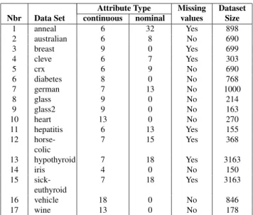
Attribute Type Missing Dataset Nbr Data Set continuous nominal values Size
1 anneal 6 32 Yes 898 2 australian 6 8 No 690 3 breast 9 0 Yes 699 4 cleve 6 7 Yes 303 5 crx 6 9 No 690 6 diabetes 8 0 No 768 7 german 7 13 No 1000 8 glass 9 0 No 214 9 glass2 9 0 No 163 10 heart 13 0 No 270 11 hepatitis 6 13 Yes 155 12 horse-colic 7 15 Yes 368 13 hypothyroid 7 18 Yes 3163 14 iris 4 0 No 150 15 sick-euthyroid 7 18 Yes 3163 16 vehicle 18 0 No 846 17 wine 13 0 No 178
Table 1: Data sets from UCI used in the experiments.
4 Experiments
4.1 Data Sets
The data sets used for the experiments were selected from the repository of databases, domain theories and data gen-erators maintained at the University of California, Irvine (http://www.ics.uci.edu/∼mlearn/MLRepository.html) [BM98]. An additional data set was used (fractal), con-sisting of 41, 616 samples extracted from an image mosaic containing 9 different textures in a texture-based image classification problem using 6 fractal features for texture characterization [VME00].
4.2 Experimental Settings
There are no standard ways to evaluate the results given by discretization algorithms. The approach used here will measure the quality of a discretization model by looking at the classification error obtained, when the discretized model obtained from an original information system is used as in-put to a machine learning algorithm targeting the decision attribute. In order to asses both the performance of ES-based discretizations, as well as some of its properties, three kinds of experiments were conducted: 1) comparison be-tween classification errors obtained with machine learning methods (ID3, C4.5 and C4.5-rules) applied to discretiza-tions obtained with the ChiMerge, MDLP methods and the ES approach on selected data sets, 2) comparison between C4.5 and ES-based discretizations for a broader range of data sets, and 3) comparison between ES discretizations with fixed criterium (rough sets in this case) but with dif-ferent selection operators.
In (1) classification errors on the decision attribute were evaluated according to three well known algorithms: ID3 [Qui86], C4.5 and C4.5-Rules [Qui96]. These methods re-quired discretized data and are appropriate for comparison purposes, done in the following way: The chosen data sets were Iris, Wine, Bupa (Table 1), and Fractal. For each data set a classical discretization technique was applied to each
non-decision attribute, and the discretized data was classi-fied with the machine learning algorithms mentioned above. The average number of classes per attribute was computed for the two models given by the ChiMerge and the MDLP methods, and that number was used as the maximal number of categories per attribute achievable during the ES-based discretizations. This approach is actually very conservative and clearly biased in favor of the classical methods used, as maybe a better solution with the ES-RS, ES-JE and ES-C4.5 algorithms could be obtained by allowing these algorithms to explore more elaborate models w.r.t. the one given ob-tained with ChiMerge and MDLP.
ES-based discretizations were computed after 25 gener-ations using (µ,λ)-selection with µ = 50 and λ = 350. Linear probability distribution was used for the selection of new parents, and recombination was set to fitness-based-scan [BFM97], which usually gives good performance in function optimizations. The elements of the ~σ vectors were in the [0.001 − 0.1] range and no rotation angle vectors ~α were used.
In Experiment 2), the combined discretization-classification of the C4.5 algorithm was compared with a discretization using ES with C4.5 fitness as criterium (ES-C4.5) (See Table 3), and a classification given by the C4.5 algorithm itself. In other words, the classification algorithm and the fitness criterium were according to the C4.5 algorithm, and only an ES-based discretization makes the difference. (µ + λ) and (µ, λ) were used, with µ = 150 and λ = 350. ~σ and ~α vectors were set as above and an average of 20 generations were used. All evaluations (5-fold cross-validation classification errors) were computed with the WEKA platform [WF99] for all the data sets described in Table 1.
In Experiment 3) the purpose was to observe the be-havior of the mean number of categories/attribute resulting from ES-based discretizations when using different selec-tion mechanisms. The rough set criterium was fixed and the RSL library [GS94] was used as the evaluation platform. ES parameters were as in Experiment 2) above.
5 Results
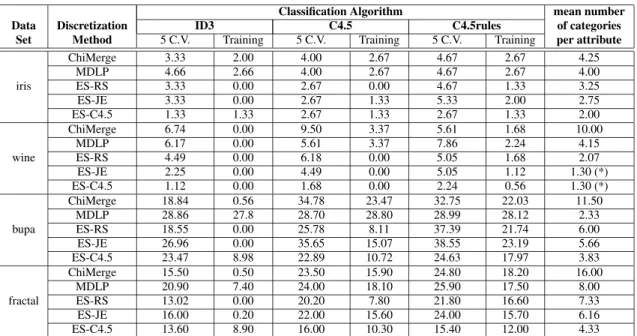
The results obtained for Experiment 1) are shown in Table 2 (classification errors for the training set are included as ref-erence). In absolute terms, 5-fold cross- validation shows that for all data sets and all the classification algorithms, the smallest errors are obtained when ES-based discretiza-tion data are used. In some cases the errors between the classical and ES-based techniques are several times higher (for example, ChiMerge vs. ES-C4.5 for Wine classifying with ID3, MDLP vs. ES-C4.5 for Iris, also with ID3, or MDLP vs. ES-C4.5 for Wine, with the C4.5 rules classi-fier). With few exceptions, the best over-all discretizations are obtained with Evolution Strategies using the C4.5 fit-ness criterium (ES-C4.5 algorithm). The training set results suggests that ES-RS and ES-JE are probably more prone to overfitting the models. As explained in the previous sec-tion, all ES-based algorithms were not allowed to generate discretizations with a number of categories/attribute higher
Classification Algorithm mean number Data Discretization ID3 C4.5 C4.5rules of categories
Set Method 5 C.V. Training 5 C.V. Training 5 C.V. Training per attribute ChiMerge 3.33 2.00 4.00 2.67 4.67 2.67 4.25 MDLP 4.66 2.66 4.00 2.67 4.67 2.67 4.00 iris ES-RS 3.33 0.00 2.67 0.00 4.67 1.33 3.25 ES-JE 3.33 0.00 2.67 1.33 5.33 2.00 2.75 ES-C4.5 1.33 1.33 2.67 1.33 2.67 1.33 2.00 ChiMerge 6.74 0.00 9.50 3.37 5.61 1.68 10.00 MDLP 6.17 0.00 5.61 3.37 7.86 2.24 4.15 wine ES-RS 4.49 0.00 6.18 0.00 5.05 1.68 2.07 ES-JE 2.25 0.00 4.49 0.00 5.05 1.12 1.30 (*) ES-C4.5 1.12 0.00 1.68 0.00 2.24 0.56 1.30 (*) ChiMerge 18.84 0.56 34.78 23.47 32.75 22.03 11.50 MDLP 28.86 27.8 28.70 28.80 28.99 28.12 2.33 bupa ES-RS 18.55 0.00 25.78 8.11 37.39 21.74 6.00 ES-JE 26.96 0.00 35.65 15.07 38.55 23.19 5.66 ES-C4.5 23.47 8.98 22.89 10.72 24.63 17.97 3.83 ChiMerge 15.50 0.50 23.50 15.90 24.80 18.20 16.00 MDLP 20.90 7.40 24.00 18.10 25.90 17.50 8.00 fractal ES-RS 13.02 0.00 20.20 7.80 21.80 16.60 7.33 ES-JE 16.00 0.20 22.00 15.60 24.00 15.70 6.16 ES-C4.5 13.60 8.90 16.00 10.30 15.40 12.00 4.33
Table 2: Classification errors obtained with Evolution Strategies using Rough Set (ES-RS), Joint Entropy (ES-JE) and C4.5 criteria (ES-C4.5), in comparison with ChiMerge and MDLP. 5-CV is 5-fold cross-validation, and training, the whole data set. Three classification algorithms were used: ID3, C4.5 and C4.5 rules. See text for explanation about (*).
than the average between ChiMerge and MDLP, thus, con-straining their search. However, ES-based results were bet-ter, thus suggesting a potential for further improving these results. On the other hand, with the exception of the Bupa data set, the number of categories/attribute of the ES-based discretizations is several times smaller than those given by ChiMerge and MDLP. This is a very remarkable feature, because not only were better classification errors obtained, but also much simpler data models (and consequently sim-pler decision rules). This is crucial when the results are interpreted by human experts (humans have difficulty han-dling more than 7-9 categories simultaneously). In particu-lar, for the case of Wine data, less than 2 categories/attribute were found, indicating that some irrelevant attributes were excluded from the model. This is a very interesting feature of ES-based discretizations not present in any other method. The results obtained for Experiment 2) are shown in Ta-ble 3. The best classification error for each data set is marked with a (*), clearly indicating that ES-based dis-cretization outperforms the C4.5 algorithm in 82.4% of the data sets (14 out of 17). Moreover, C4.5 errors are greater than ES-C4.5 by an average absolute difference of 3.62 when ES-C4.5 performs better, whereas when C4.5 is better (in 17.6% of the cases), the average absolute difference is only 0.35. Within the ES, in 58.82% of the cases (consid-ering all 17), the (µ, λ) selection performs better than the (µ + λ). If data sets are investigated individually, the results from Table 3 can be improved (all ES discretizations were computed with the same set of parameters regardless of the data set used). For example, according to Table 3, the C4.5 algorithm performed better than the ES for sick-euthyroid data. However, an independent experiment using µ = 250 and a σ range of [0.01,0.1] gave an error of 1.64, better than C4.5, thus showing the potential for even better ES perfor-mance.
Classification Error Data Set Evolution Strategies
C45 (C4.5 criterium) (µ + λ) (µ, λ) anneal 2.01 1.68 1.45 * + australian 15.08 14.93 * + 15.08 breast 5.30 4.01 3.72 * + cleve 25.75 21.13 * + 21.46 crx 14.35 * 14.64 + 15.37 diabetes 27.61 21.23 * + 22.92 german 27.80 25.70 * + 25.80 glass 27.11 22.13 * + 23.84 glass2 22.70 11.05 10.43 * + heart 19.26 18.89 17.41 * + hepatitis 21.94 19.36 18.71 * + horse-colic 14.41 13.59 12.23 * + hypothyroid 0.86 * 1.11 + 1.21 iris 4.670 5.34 2.67 * + sick-euthyroid 1.97 * 2.57 2.47 + vehicle 27.90 25.42 21.87 * + wine 6.18 7.31 3.38 * + Nbr. of best 3 5 9 overall best 3 14
Table 3: Comparison of the classification accuracy in 5-fold cross-validation experiments between the C4.5 algorithm and the Evolution Strategies approach using the C4.5 cri-terium. The (*) indicates the best result for a given data set. The (+) indicates the best result within the ES variants. The last two rows shows the number of times in which the cor-responding algorithm gives the over-all best classification error.
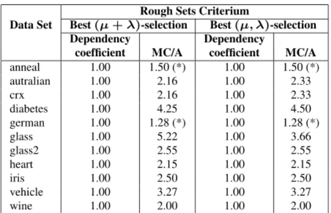
Rough Sets Criterium
Data Set Best (µ + λ)-selection Best (µ, λ)-selection Dependency Dependency
coefficient MC/A coefficient MC/A anneal 1.00 1.50 (*) 1.00 1.50 (*) autralian 1.00 2.16 1.00 2.33 crx 1.00 2.16 1.00 2.33 diabetes 1.00 4.25 1.00 4.50 german 1.00 1.28 (*) 1.00 1.28 (*) glass 1.00 5.22 1.00 3.66 glass2 1.00 2.55 1.00 2.55 heart 1.00 2.15 1.00 2.15 iris 1.00 2.50 1.00 2.50 vehicle 1.00 3.27 1.00 3.27 wine 1.00 2.00 1.00 2.00
Table 4: Simultaneous discretization with Evolution Strate-gies using the Rough Sets criterium for (µ + λ) and (µ, λ) selection mechanisms. MC/A is the mean number of cate-gories/attribute in the resulting discretization. (*) indicates values smaller than 2.
Results for Experiment 3) are shown in Table 4. All de-pendency coefficients were 1 (i.e. complete description of the classes of the decision attribute), and with the exception of data set (glass), the mean number of categories/attribute created are either the same of very close, regardless of the selection mechanism. In particular, redundant attributes were discovered for the (anneal) and (german) data sets. These preliminary results suggest that the ES-discretization is robust w.r.t the choice of the selection operator and also that it does not hamper the ability of discovering irrelevant attributes.
6 Conclusions
The results, although preliminary, show that supervised, global discretization algorithms based on Evolution Strate-gies are very effective, robust, and capable of outperform-ing classical discretization techniques in the data minoutperform-ing field. Moreover, this increased performance is obtained with discretizations having a much smaller number of cate-gories/attribute, therefore, with much simpler models. More accurate and easily interpretable models are highly pursued in Data Mining, thus, the property of ES-based discretiza-tion algorithms of discovering models of precisely this kind is a very remarkable one. In addition, it was found that ES-based discretization algorithms can detect irrelevant at-tributes as part of the discretization process (also it seems that this capability is not affected by the selection mech-anism chosen). This is a feature which is not present in classical methods. The best results are obtained when the evolution strategies-based algorithm uses as fitness a C4.5 criterium, and in general (µ, λ)-selection performs better than (µ + λ). Additional experiments targeting individual data sets show that there is still potential for increased ES performance. Further investigations are necessary in order to study the properties and possibilities of this approach, considering that only a small number of ES operators were used, thus leaving a potential for possibly better results.
7 Acknowledgments
This work is supported by the Mexican Institute of Petroleum, the Spanish project CICyT DPI2002-03225 and by the National Research Council of Canada.
Bibliography
[And73] M. Anderberg, Cluster Analysis for Applica-tions, John Wiley & Sons, London UK, 1973. [Bac91] T. Back, Evolutionary Algorithms in Theory
and Practice, Oxford University Press, Ox-ford, 1991.
[BFM97] T. Back, D. Fogel, and Z. Michalewicz, Hand-book of Evolutionary Computation, Oxford University Press, Oxford, 1997.
[BM98] C. L. Blake and C.J. Merz, UCI Repository of Machine Learning Databases, 1998.
[CN89] P. Clark and T. Niblett, The CN2 Induction Al-gorithm, Machine Learning 9 (1989), no. 1,
57–94.
[FI93] U. M. Fayyad and K. B. Irani, Multi-interval Discretization of continuous-valued Attributes for Classification Learning, In Proc. 13th In-ternational Conference on Machine Learn-ing, Morgan Kaufmann Publishers, 1993, pp. 1022–1027.
[FKY96] J. Friedman, R. Kohavi, and Y. Yun, Lazy De-cision Trees, In Proc. 13th National Confer-ence on Artificial IntelligConfer-ence, AAAI Press and the MIT Press, 1996.
[GS94] M. Gawrys and J. Sienkiewicz, Rough Sets Library version 2.0, Tech. Report ICS TUW Research Report 27/94, Warsaw University of Technology, September 1994.
[Ker92] R. Kerber, ChiMerge: Discretization of Nu-meric Attributes, In Proc. 10th National Con-ference on Artificial Intelligence, MIT Press, 1992, pp. 123–128.
[MRMC00] L. C. Molina, S. Rezende, M. C. Monard, and C. Caulkins, Transforming a Regression Problem into a Classification Problem using Hybrid Discretization, Revista Computaci´on y Sistemas CIC-IPN4 (2000), no. 1, 44–52.
[Paw82] Z. Pawlak, Rough Sets, International Jour-nal of Information and Computer Sciences11
(1982), 341–356.
[Paw91] , Rough Sets, Theoretical Aspects of Reasoning about Data, Kluwer Academic Publishers, New York, 1991.
[Qui86] J. R. Quinlan, Induction of Decision Trees, Machine Learning1 (1986), 81–106.
[Qui89] , Inferring Decision Trees using the Minimum Description Length Principle, In-formation and Computation80 (1989), no. 3,
227–248.
[Qui96] , Learning First-Order Definitions of Functions, Journal of Artificial Intelligence Research5 (1996), 139–161.
[Rec73] I. Rechenberg, Evolutionsstrategien: Opti-mierung Technischer Systeme nach Prinzip-ien der Biologischen Evolution, Frommann-Holzboog, Stuttgart, 1973.
[Ris86] J. Rissanen, Stochastic Complexity and Mod-elling., Ann. Statist 14 (1986), no. 1, 1080–
1100.
[Sch81] H. P. Schwefel, Numerical Optimization of Computer Models, John Wiley & Sons, Chich-ester, 1981.
[VME00] J. J. Vald´es, L. C. Molina, and S. Espinosa, Characterizing Fractal features for Texture Description in Digital Images: an Experi-mental Study, Proc. 15th International Con-ference on Pattern Recognition, Barcelona, Spain, vol. 3, IEEE Computer Society, 2000, pp. 917–920.
[VMP00] J. J. Vald´es, L. C. Molina, and N. Peris, Si-multaneous Supervised Discretization of Nu-meric Attributes: a Soft Computing Approach (draft), Tech. report, LSI-UPC, Barcelona, Spain, 2000.
[WF99] I. H. Witten and E. Frank, Data Mining: Practical Machine Learning Tools and Tech-niques with Java Implementations, Morgan Kaufmann Publishers, 1999.
[YL97] X. Yao and Y. Liu, Fast Evolution Strategies, Evolutionary Programming VI (Berlin) (P. J. Angeline, R. G. Reynolds, J. R. McDonnell, and R. Eberhart, eds.), Springer Verlag, 1997, pp. 151–161.