HAL Id: hal-03048455
https://hal.archives-ouvertes.fr/hal-03048455
Submitted on 10 Dec 2020
HAL is a multi-disciplinary open access
archive for the deposit and dissemination of
sci-entific research documents, whether they are
pub-lished or not. The documents may come from
teaching and research institutions in France or
abroad, or from public or private research centers.
L’archive ouverte pluridisciplinaire HAL, est
destinée au dépôt et à la diffusion de documents
scientifiques de niveau recherche, publiés ou non,
émanant des établissements d’enseignement et de
recherche français ou étrangers, des laboratoires
publics ou privés.
The influence of foreign vs. North American emissions
on surface ozone in the US
D. Reidmiller, A. Fiore, D. Jaffe, D. Bergmann, C. Cuvelier, F. Dentener, B.
Duncan, G. Folberth, M. Gauss, S. Gong, et al.
To cite this version:
D. Reidmiller, A. Fiore, D. Jaffe, D. Bergmann, C. Cuvelier, et al.. The influence of foreign vs.
North American emissions on surface ozone in the US. Atmospheric Chemistry and Physics, European
Geosciences Union, 2009, 9 (14), pp.5027-5042. �10.5194/ACP-9-5027-2009�. �hal-03048455�
www.atmos-chem-phys.net/9/5027/2009/ © Author(s) 2009. This work is distributed under the Creative Commons Attribution 3.0 License.
Chemistry
and Physics
The influence of foreign vs. North American emissions on surface
ozone in the US
D. R. Reidmiller1,2, A. M. Fiore3, D. A. Jaffe2, D. Bergmann4, C. Cuvelier5, F. J. Dentener5, B. N.Duncan6,*,
G. Folberth7, M. Gauss8, S. Gong9, P. Hess10,**, J. E. Jonson11, T. Keating12, A. Lupu13, E. Marmer5, R. Park14,***,
M. G. Schultz15, D. T. Shindell16, S. Szopa17, M. G. Vivanco18, O. Wild19, and A. Zuber20
1University of Washington, Department of Atmospheric Sciences, Seattle, WA, USA
2University of Washington – Bothell, Department of Interdisciplinary Arts and Sciences, Bothell, WA, USA
3NOAA Geophysical Fluid Dynamics Laboratory, Princeton, NJ, USA
4Atmospheric Earth and Energy Division, Lawrence Livermore National Laboratory, Livermore, CA, USA
5European Commission, Joint Research Centre JRC, Institute for Environment and Sustainability, Ispra, Italy
6Goddard Earth Sciences & Technology Center, UMBC, MD, USA
7Ecole Polytechnique F´ed´erale de Lausanne (EPFL), Lausanne, Switzerland
8Department of Geosciences, University of Oslo, Oslo, Norway
9Science and Technology Branch, Environment Canada, Toronto, ON, Canada
10National Center for Atmospheric Research, Boulder, CO, USA
11Norwegian Meteorological Institute, Oslo, Norway
12Office of Policy Analysis and Review, EPA, Washington, DC, USA
13Center for Research in Earth and Space Science, York University, Toronto, ON, Canada
14Atmospheric Chemistry Modeling Group, Harvard University, Cambridge, MA, USA
15ICG-2, Forschungszentrum J¨ulich, J¨ulich, Germany
16NASA Goddard Institute for Space Studies and Columbia University, New York, NY, USA
17Laboratoire des Sciences du Climat et de l’Environnement, CEA/CNRS/UVSQ/IPSL, Gif-sur-Yvette, France
18Centro de Investigaciones Energ´eticas, Medioambientales y Tecnol´ogicas (CIEMAT), Madrid, Spain
19Lancaster Environment Centre, Lancaster University, Lancaster, UK
20Environment Directorate General, European Commission, Brussels, Belgium
*now at: NASA Goddard Space Flight Center, Greenbelt, MD, USA
**also at: Cornell University, Ithaca, New York, USA
***now at: Seoul National University, Seoul, Korea
Received: 23 February 2009 – Published in Atmos. Chem. Phys. Discuss.: 25 March 2009 Revised: 18 June 2009 – Accepted: 15 July 2009 – Published: 27 July 2009
Abstract. As part of the Hemispheric Transport of Air Pol-lution (HTAP; www.htap.org) project, we analyze results from 15 global and 1 hemispheric chemical transport mod-els and compare these to Clean Air Status and Trends Net-work (CASTNet) observations in the United States (US) for 2001. Using the policy-relevant maximum daily 8-h
aver-age ozone (MDA8 O3) statistic, the multi-model ensemble
represents the observations well (mean r2=0.57, ensemble
bias = +4.1 ppbv for all US regions and all seasons) despite a wide range in the individual model results. Correlations
Correspondence to: D. R. Reidmiller ([email protected])
are strongest in the northeastern US during spring and fall
(r2=0.68); and weakest in the midwestern US in summer
(r2=0.46). However, large positive mean biases exist
dur-ing summer for all eastern US regions, rangdur-ing from 10– 20 ppbv, and a smaller negative bias is present in the western US during spring (∼3 ppbv). In nearly all other regions and seasons, the biases of the model ensemble simulations are
≤5 ppbv. Sensitivity simulations in which anthropogenic O3
-precursor emissions (NOx+ NMVOC + CO + aerosols) were
decreased by 20% in four source regions: East Asia (EA), South Asia (SA), Europe (EU) and North America (NA)
show that the greatest response of MDA8 O3to the summed
West (0.9 ppbv reduction due to 20% emissions reductions from EA + SA + EU). East Asia is the largest contributor to
MDA8 O3at all ranges of the O3 distribution for most
re-gions (typically ∼0.45 ppbv) followed closely by Europe. The exception is in the northeastern US where emissions reductions in EU had a slightly greater influence than EA
emissions, particularly in the middle of the MDA8 O3
dis-tribution (response of ∼0.35 ppbv between 35–55 ppbv). EA and EU influences are both far greater (about 4×) than that from SA in all regions and seasons. In all regions and
sea-sons O3-precursor emissions reductions of 20% in the NA
source region decrease MDA8 O3the most – by a factor of
2 to nearly 10 relative to foreign emissions reductions. The
O3response to anthropogenic NA emissions is greatest in the
eastern US during summer at the high end of the O3
distri-bution (5–6 ppbv for 20% reductions). While the impact of
foreign emissions on surface O3in the US is not negligible –
and is of increasing concern given the recent growth in Asian emissions – domestic emissions reductions remain a far more
effective means of decreasing MDA8 O3values, particularly
those above 75 ppb (the current US standard).
1 Introduction
It is well-established that the intercontinental transport of pollutant emissions affects surface air quality in the United States (Berntsen et al., 1999; Jacob et al., 1999; Jaffe et al., 1999; Fiore et al., 2002; Goldstein et al., 2004; Keating et al., 2005; Sudo and Akimoto, 2007; Lin et al., 2008; Oltmans et al., 2008; Zhang et al., 2008; Fischer et al., 2009). Transport “events” can lead to exceedances in air quality standards for downwind regions (Jaffe et al., 2004). As a result, foreign emissions can significantly affect the health of humans and crops in the US (Bell et al., 2004; Ellingsen et al., 2008; Casper-Anenberg et al., 2009). However, the effect foreign emissions have on air quality in the US can vary significantly on time-scales from days (Yienger et al., 2000; Liang et al., 2007) to months (Liu et al., 2003; Liang et al., 2004; Weiss-Penzias et al., 2004; Wang et al., 2006) to years (Liang et al., 2005; Liu et al., 2005; Reidmiller et al., 2009).
Over the past 15 years, a multitude of field campaigns have attempted to quantify the effect of Asian emissions on US air quality and how these emissions are affecting the pho-tochemical environment over the North Pacific. The Pacific Exploratory Mission – West phase (PEM-West; Hoell et al., 1997) took place in 1994 to study the chemical outflow from East Asian emissions. The Photochemical Ozone Budget of the Eastern North Pacific Atmosphere (PHOBEA; Jaffe et al., 2001; Kotchenruther et al., 2001; Bertschi et al., 2004) cam-paign was a multi-year investigation spanning 1997–2002 using aircraft and ground measurements to quantify the im-pacts of Asian emissions on pollutant inflow to the north-western US. The Transport and Chemical Evolution over the
Pacific (TRACE-P; Jacob et al., 2003) and Intercontinental Transport and Chemical Transformation (ITCT 2K2; Parrish et al., 2004a; Goldstein et al., 2004) campaigns were con-ducted during spring - the season of greatest East Asian trans-port to North America – of 2001 and 2002, respectively. In 2004, the Pacific Exploration of Asian Continental Emission (PEACE; Parrish et al., 2004a) experiment was carried out in two phases over winter and spring to determine seasonal differences in transpacific transport and photochemical en-vironments. Also in 2004, a remote free tropospheric site near the US west coast was established atop Mt. Bachelor in
central Oregon (43.98◦N, 121.69◦W; 2.7 km a.s.l.) allowing
frequent observations of Asian pollution plumes in the US (Weiss-Penzias et al., 2006; Swartzendruber et al., 2006). Most recently, in spring 2006, the Intercontinental Chem-ical Transport Experiment (INTEX-B; Singh et al., 2009) was a coordinated satellite, aircraft and ground-based cam-paign designed in large part to quantify the import of Asian pollutants to western North America. Additionally, satellite data are now being used to better understand and quantify the intercontinental transport of pollutants (Heald et al., 2003; Damoah et al., 2004; Creilson et al., 2003; Wenig et al., 2003).
Similarly, North American emissions affect air quality
in downwind regions, as well. The North Atlantic
Re-gional Experiment (NARE) and the International Consortium for Atmospheric Research on Transport and Transformation (ICARTT) both quantified the outflow of North American emissions and their impacts on downwind regions (Parrish et al., 2004b; Li et al., 2004; Hudman et al., 2007). Along a similar vein, Cooper et al. (2005) used ozonesonde and MOZAIC aircraft data to quantify transport pathways on the inflow (west coast) and outflow (east coast) regions of the US. Li et al. (2002) found that North American
anthro-pogenic emissions enhance surface O3in continental Europe
by 2–4 ppbv on average during summer and by 5–10 ppbv during trans-Atlantic transport events.
Beyond field campaigns and satellite observations, global chemical transport models (CTMs) are valuable tools with which we can quantify the intercontinental transport of pol-lution. While the existing literature on this topic is expansive (e.g., Klonecki and Levy, 1997; Jacob et al., 1999; Yienger et al., 1999, 2000; Fiore et al., 2002, 2003; Liang et al., 2004, 2005, 2007; Auvray et al., 2007; Lin et al., 2008), there is a lack of coherency in these individual modeling studies that makes it difficult to draw any meaningful conclusions
about the magnitude of the foreign influence on surface O3
in the US. In response to this, the UN Economic Commis-sion for Europe’s Convention on Long-Range Transbound-ary Air Pollution developed the Task Force on Hemispheric Transport of Air Pollution (TF HTAP; http://www.htap.org) in December 2004. A major TF HTAP activity was to de-sign a set of simulations that were executed by 20+ modeling groups in an effort to quantify the source-receptor
persistent organic pollutants (TF HTAP, 2007). Its objectives are to understand the key processes governing intercontinen-tal transport, quantify source-receptor relationships and iden-tify future research needs. In addition to the HTAP interim report (TF HTAP, 2007), several studies have utilized this valuable data set: Sanderson et al. (2008) investigate how nitrogen deposition is affected by intercontinental transport; Shindell et al. (2008) determine source attribution for pollu-tants transported to the Arctic; Fiore et al. (2009) quantify
the source-receptor relationships for ground-level O3
pollu-tion using four northern hemispheric (NH) regions – East Asia (EA), South Asia (SA), Europe (EU) and North Amer-ica (NA); Casper-Anenberg et al. (2009) estimate the
mortal-ities avoided by 20% reductions of anthropogenic O3
precur-sor emissions in the four source regions; Jonson et al. (2009)
investigate the ability of the models to capture vertical O3
distributions as measured by ozonesondes and intercontinen-tal contribution throughout the atmospheric column.
Our objectives are to: (1) assess the multi-model skill in
reproducing the observed maximum daily 8-h average O3
(MDA8 O3) statistic, (2) determine the contribution from
intercontinental sources to surface O3 in the US, and (3)
compare foreign vs. NA influences on MDA8 O3 and how
this relationship varies by region, season and across the O3
distribution. The method adopted here begins by
select-ing regionally-representative CASTNet sites, puttselect-ing obser-vations from 2001 (the year of the HTAP simulations) in
con-text with climatological O3behavior (Sect. 2.1) and briefly
describing the global models used (Sect. 2.2). We then assess the ability of the multi-model mean to reproduce observed
MDA8 O3in various regions on seasonal, monthly and daily
timescales (Sect. 3). Finally, we use the perturbation sim-ulations in which NA and foreign (i.e., EA + SA + EU)
an-thropogenic O3-precursor emissions were reduced by 20%
to quantify the differences between foreign (Sect. 4) vs.
do-mestic sources (Sect. 5) on MDA8 O3throughout the US in
different seasons and across the O3distribution.
2 Methodology
2.1 CASTNet observations
As required by the Clean Air Act Amendments of 1990, CASTNet was developed by the US Environmental Protec-tion Agency (EPA) in order to establish an effective, ru-ral monitoring and assessment network at locations away from pollutant emission sources and heavily populated ar-eas (US EPA, 2008; Eder et al., 2005). Monitoring locations were selected according to strict siting criteria designed to avoid undue influence from point sources, area sources and local activities. As a result, most CASTNet sites are located in rural areas with open, rolling terrain, well-removed from emission sources (Holland et al., 1999; Tong and Mauzerall, 2006).
The primary purpose of CASTNet is to identify and char-acterize broad-scale spatial and temporal trends of various air pollutants and their environmental effects (Eder et al., 2005). The network was developed from the existing Na-tional Dry Deposition Network and has become the nation’s primary monitoring network for measuring concentrations of
rural ambient (background) O3 levels. A selection of
stud-ies using CASTNet O3 data include investigations of:
sub-grid segregation on ozone production efficiency in a chem-ical model (Liang and Jacobson, 2000); variability in
sur-face background O3throughout the US (Lefohn et al., 2001;
Fiore et al., 2003); and the positive trend in O3 throughout
the western US (Jaffe and Ray, 2007).
Figure 1 illustrates the 83 currently operational CASTNet sites. Table A1 lists the geographic information (latitude, longitude and elevation) for these CASTNet sites. We divide the US into nine broad geographic regions based on bound-aries of the EPA’s 10 Regions, CASTNet site density and ba-sic geographical and topographical features. Since the HTAP project uses CTMs with typical resolutions of 100–500 km, we attempt to use the CASTNet observations in a manner representative of these large spatial scales. As a result, we determine “regionally-representative” sites through a unique methodology, but with a similar goal and outcome to that of Lehman et al. (2004) and Fuentes (2003).
We calculate monthly mean MDA8 O3 for each of the
68 sites with nearly complete records in 2001 (≥21 days of data per month; Figs. 2 and A1). (Note, from here on-ward we compare the Mountain West and Southeast regions in this article to show differences in East vs. West US re-gions; results from the other seven regions are in the Aux-iliary Materials: http://www.atmos-chem-phys.net/9/5027/ 2009/acp-9-5027-2009-supplement.pdf) Averaging all the sites within a given region (open circles in Fig. 2), we de-termine a “regional mean” (solid gray triangles) annual
cy-cle of MDA8 O3. We then calculate: (1) r2values between
each site and the regional mean, as well as (2) the summa-tion of the monthly mean deviasumma-tions for each site from the regional mean. Each site is then assigned a ranking based on these two metrics. The rankings are then summed for each site (e.g., a ranking of “1” was assigned to the site with the highest correlation and also to the site with the lowest summed deviation for a cumulative ranking of “2”). The sites with the lowest summed ranking were classified as “regionally-representative” (stars in Fig. 1 and bold entries in Table A1). If the number of sites within a given region is <5, then 2 regionally-representative sites are chosen; if 5–12 sites are in a region, then 3 representative sites are cho-sen; if >12 sites are in a region, then 4 representative sites are chosen. For the California region, it is difficult to clas-sify regionally-representative sites due to the widely varying topography, meteorology and influence of local emissions (California Air Resources Board, 2001); we selected Death Valley (DEV) and Yosemite (YOS) National Park sites
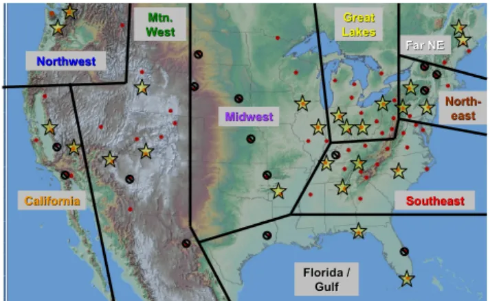
Figure 1. Map of the 83 CASTNet sites (red dots) in the U.S. Geographic regions used
in our analysis for the year 2001 are divided with black lines. “Regionally-representative” sites are highlighted with stars (criteria discussed in Section 2.1). Sites with more than 30 consecutive days of missing data for 2001 (and therefore excluded from our analysis) are denoted by black circles with lines through them.
Northwest Northwest California California Plains Plains Southeast Southeast Great Great Lakes Lakes North North- -east east Mtn Mtn. . West West Florida / Florida / Gulf Gulf Far NE Far NE Northwest Northwest California California Plains Plains Southeast Southeast Great Great Lakes Lakes North North- -east east Mtn Mtn. . West West Florida / Florida / Gulf Gulf Far NE Far NE Northwest Northwest California California Plains Plains Southeast Southeast Great Great Lakes Lakes North North- -east east Mtn Mtn. . West West Florida / Florida / Gulf Gulf Far NE Far NE Northwest Northwest California California Plains Plains Southeast Southeast Great Great Lakes Lakes North North- -east east Mtn Mtn. . West West Florida / Florida / Gulf Gulf Far NE Far NE Midwest Midwest Northwest Northwest California California Plains Plains Southeast Southeast Great Great Lakes Lakes North North- -east east Mtn Mtn. . West West Florida / Florida / Gulf Gulf Far NE Far NE Northwest Northwest California California Plains Plains Southeast Southeast Great Great Lakes Lakes North North- -east east Mtn Mtn. . West West Florida / Florida / Gulf Gulf Far NE Far NE Midwest Midwest
Fig. 1. Map of the 83 CASTNet sites (red dots) in the US. Geo-graphic regions used in our analysis for the year 2001 are divided with black lines. “Regionally-representative” sites are highlighted with stars (criteria discussed in Sect. 2.1). Sites with more than 30 consecutive days of missing data for 2001 (and therefore ex-cluded from our analysis) are denoted by black circles with lines through them.
because they represent site elevation extremes and had the best rankings.
We compare MDA8 O3values for 2001 with the CASTNet
climatology over the 1989–2004 period to examine whether 2001 was representative of typical conditions. Results for all years are illustrated in Fig. 3 for the Mountain West and Southeast regions (Fig. A2 shows the other 7 regions). From a policy-perspective, we are concerned with the
num-ber of exceedances days (when MDA8 O3>75 ppbv).
Ta-ble 1 shows the climatology (through 2004) of exceedance days for each site within a region. Exceedance days for the “Region” are determined by calculating the number of ex-ceedances for each regionally representative site and then av-eraging these values for a given region. Using the current
US EPA standard of the 4th highest MDA8 O3>75 ppbv to
classify an exceedance of the air quality standard, Table 1 shows that sites in the California, Midwest, Great Lakes, Northeast and Southeast regions are regularly in exceedance. To put the values from Fig. 3 (and Fig. A2) and Table 1
in context, we calculate seasonal mean MDA8 O3values and
compare them to the climatological values (through 2004) in Table 2. We define a ±3% threshold deviation from the climatology to classify the season as “non-normal”. Only
one season in one region had a seasonal mean MDA8 O3
value that was >1σ (where σ indicates standard deviation) from the climatological mean for that season (MAM in the Far Northeast). During summer (JJA), all regions had
MDA8 O3 values that were at or below normal, with the
Southeast (−1.4 ppbv or −3.7%), Florida/Gulf (−2.2 ppbv or
−7.2%) and Great Lakes (−2.8 ppbv or −6.2%) regions
ex-hibiting the greatest below-normal deviations. The East coast (with the exception of the Florida/Gulf region) experienced
an above-normal O3 season in autumn (SON), while the
northernmost regions (Northwest and Far Northeast regions)
Figure 2. Monthly mean MDA8 O3 at the individual CASTNet sites (open circles) and
the multi-site regional mean (solid gray triangles) in the (a) Mountain West and (b) Southeast regions. Regionally-representative sites for the Mountain West region are Mesa Verde NP, CO (MEV), Pinedale, WY (PND) and Grand Canyon NP, AZ (GRC); and Cadiz, KY (CDZ), Candor, NC (CND), Sand Mountain, AL (SND) and Speedwell, TN (SPD) for the Southeast region; the mean of these regionally-representative sites is depicted with solid red triangles. Geographic information and 3-letter abbreviations for all sites are listed in Table A1. Note the difference in the range of the y-axes between the two regions. M D A 8 O 3 (p p b v ) 35 40 45 50 55 60 65 J F M A M J J A S O N D CNT GTH GRB MEV PND YEL GRC CAN CHA Reg. Mean Reg. Repr. Mountain West (a) 15 25 35 45 55 65 J F M A M J J A S O N D BEL BWR VPI PED SHN CDZ CKT MCK ESP GRS SPD COW PNF BFT CND SND CVL GAS Reg. Mean Reg. Repr. Southeast Region (b) M D A 8 O 3 (p p b v ) 35 40 45 50 55 60 65 J F M A M J J A S O N D CNT GTH GRB MEV PND YEL GRC CAN CHA Reg. Mean Reg. Repr. Mountain West (a) 35 40 45 50 55 60 65 J F M A M J J A S O N D CNT GTH GRB MEV PND YEL GRC CAN CHA Reg. Mean Reg. Repr. Mountain West (a) 15 25 35 45 55 65 J F M A M J J A S O N D BEL BWR VPI PED SHN CDZ CKT MCK ESP GRS SPD COW PNF BFT CND SND CVL GAS Reg. Mean Reg. Repr. Southeast Region (b) 15 25 35 45 55 65 J F M A M J J A S O N D BEL BWR VPI PED SHN CDZ CKT MCK ESP GRS SPD COW PNF BFT CND SND CVL GAS Reg. Mean Reg. Repr. Southeast Region (b)
Fig. 2. Monthly mean MDA8 O3at the individual CASTNet sites (open circles) and the multi-site regional mean (solid gray triangles) in the (a) Mountain West and (b) Southeast regions. Regionally-representative sites for the Mountain West region are Mesa Verde NP, CO (MEV), Pinedale, WY (PND) and Grand Canyon NP, AZ (GRC); and Cadiz, KY (CDZ), Candor, NC (CND), Sand Mountain, AL (SND) and Speedwell, TN (SPD) for the Southeast region; the mean of these regionally-representative sites is depicted with solid red triangles. Geographic information and 3-letter abbreviations for all sites are listed in Table A1. Note the difference in the range of the y-axes between the two regions.
Figure 3. Climatology of monthly mean MDA8 O3 for the mean of the
regionally-representative sites in the (a) Mountain West and (b) Southeast regions. Solid red triangles indicate the HTAP year of 2001(and represent the same data shown as solid red triangles as in Fig. 2); solid black triangles depict the multi-year average climatology. Datapoints are missing if <21 days of MDA8 O3 data exist for that month. Note the
difference in the range of the y-axes between the two regions.
M D A 8 O 3 (p p b v ) 1989 1990 1991 1992 1993 1994 1995 1996 1997 1998 1999 2000 2001 2002 2003 2004 Mean 30 35 40 45 50 55 60 65 70 J F M A M J J A S O N D 20 30 40 50 60 70 J F M A M J J A S O N D (a) (b)
Mountain West Region
Southeast Region M D A 8 O 3 (p p b v ) 1989 1990 1991 1992 1993 1994 1995 1996 1997 1998 1999 2000 2001 2002 2003 2004 Mean 30 35 40 45 50 55 60 65 70 J F M A M J J A S O N D 20 30 40 50 60 70 J F M A M J J A S O N D (a) (b)
Mountain West Region
Southeast Region
Fig. 3. Climatology of monthly mean MDA8 O3for the mean of the regionally-representative sites in the (a) Mountain West and (b) Southeast regions. Solid red triangles indicate the HTAP year of 2001 (and represent the same data shown as solid red triangles as in Fig. 2); solid black triangles depict the multi-year average climatol-ogy. Datapoints are missing if <21 days of MDA8 O3data exist for that month. Note the difference in the range of the y-axes between the two regions.
also saw anomalously high O3seasons in spring (MAM) at +11.1% (+5.4 ppbv) and +5.8% (+4.5 ppbv), respectively.
2.2 Model simulations
Sixteen CTMs (Table A2) provided hourly surface ozone for a “base-case” year 2001 simulation from which we
calcu-lated MDA8 O3 for our analysis. Tables 1 and A1–A3 in
Fiore et al. (2009) describe meteorological fields and emis-sions inventories used by the 16 CTMs for the HTAP simu-lations. Methane concentrations were set to a uniform mix-ing ratio of 1760 ppb, while each modelmix-ing group was asked
to employ their best estimate of O3-precursor emissions for
2001 and a minimum initialization time of six months to al-low the simulated trace gas concentrations to fully respond to the imposed perturbation.
Relative to the base-case simulations, perturbation exper-iments were conducted by 12 of the modeling groups
(de-noted by # in Table A2) in which anthropogenic O3-precursor
emissions (NOx, NMVOC, CO and aerosols) were reduced
by 20% in each of the four source regions depicted in Fig. A3
(EA, SA, EU and NA). We estimate the MDA8 O3response
to simultaneous reductions in multiple source regions as the
sum of the O3responses to the individual regional reductions
(e.g., EA + SA + EU). The 20% emissions reduction repre-sents a policy-relevant possibility, as well as a compromise
between producing a detectable response in the O3
simula-tions and applying a sufficiently small perturbation to allow the results to be scaled linearly to perturbations of different magnitudes (Fiore et al., 2009). The applicability of scaling
and linearity of an O3response to changes in precursor
emis-sions with respect to the HTAP experiments is discussed in further detail by Wu et al. (2009). In our analysis all models were sampled at the lowest model level in the grid cell con-taining the measurement site. We present uncertainty as 1σ of the multi-model mean unless otherwise stated, where σ is calculated from the simulated values at each site. The spread across models is just one metric for quantifying the uncer-tainty in a multi-model ensemble (Fiore et al., 2009). The model values are determined in a way directly analogous to
the CASTNet observations: daily regional mean MDA8 O3
values represent the average of the values at each of the re-gionally representative sites.
3 Model evaluation with CASTNet observations
Utilizing observations alone to directly determine “sensitiv-ities” (i.e., responses to emissions changes) is very difficult. Such efforts have been made at elevated free tropospheric sites like the Mt Bachelor Observatory (Weiss-Penzias et al., 2006) using the 1Hg/1CO enhancement ratio as a metric for quantifying the Asian contribution to air sampled in the US. However, similar studies at lower elevation sites (e.g., Gold-stein et al., 2004; Fischer et al., 2009) concluded that it is
very difficult to elucidate a foreign contribution signal unless there are events of very large magnitude. As a result, mod-eling experiments such as the HTAP simulations are essen-tial to understand the more continuous, lower-signal foreign contribution to air quality in downwind regions. Future work is needed to design/determine observations that can be used to directly test the model capability to capture the ozone re-sponse to emissions perturbations (i.e., the sensitivity rather than simply total ozone)
Many of the models used here have been extensively
evaluated against O3observations in previous publications.
We summarize the results from recent multi-model evalua-tion efforts in which many of the same models participated.
Ellingsen et al. (2008) compared O3 concentrations from
18 models (10 of which are used in this study) to surface observations and found that levels and seasonality were re-produced well and that annual average biases were ≤5 ppbv for regions in North America and Europe, but were larger (15–20 ppbv) in some regions where observations were more sparse. Stevenson et al. (2006) evaluated 26 models (10 of which are used in this study) with global ozonesonde mea-surements and found that the multi-model mean closely re-sembled the observations (within 1σ of each other). They also showed that the multi-model mean tended to
underesti-mate the amplitude of the seasonal cycle at 30–90◦N,
over-estimating winter O3by ∼10 ppbv.
To our knowledge, this is the first evaluation of multiple global models with observed metrics relevant for air
qual-ity (i.e., MDA8 O3). It is essential to understand how well
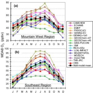
the models reproduce the observations before interpreting the perturbation simulation results. Figure 4 shows monthly
mean MDA8 O3from each of the 16 CTMs, the CASTNet
observations, and the multi-model mean for the Mountain West and Southeast regions (Fig. A4 illustrates the model evaluation for the other seven regions). Recall, here (and onward) we present regional values as averages of the obser-vations from regionally-representative sites and the models sampled at those sites. The multi-model mean represents the observations quite well in most regions during most seasons
with a mean r2=0.57 (average of all multi-model mean vs.
observations correlations in Table 3 in all regions and sea-sons), although the individual models span a wide range (76– 145% of observations during spring in the Mountain West and 77–151% of observations in the Southeast during au-tumn). The greatest model spread occurs during summer for most regions (modeled values are 45–227% of observations depending on the region). In most cases, a given model per-forms similarly across all regions (i.e., if it overestimates servations in the Mountain West, it also overestimates
ob-servations in the Southeast and elsewhere). A review of
CTM studies of tropospheric O3found that cross-tropopause
transport, deposition, humidity and lightning all contribute to inter-model differences (Wild, 2007). Near the surface, uncertainties in deposition, humidity and isoprene chemistry are probably driving the inter-model spread shown here.
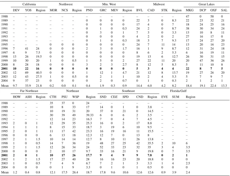
Table 1. Climatology of exceedance days for each region (defined as MDA8 O3>75 ppbv). Exceedance days for “Region” are determined by averaging the number of exceedance days from each regionally representative site in that region. Site-specific exceedance days occur when the daily MDA8 O3>75 ppbv for that site.
California Northwest Mtn. West Midwest Great Lakes
DEV YOS Region MOR NCS Region PND GRC MEV Region BVL CAD STK Region MKG DCP OXF SAL
1988 – – – – – – – – – – – – – – 47 0 58 0 1989 – – – – – – 0 0 0 0 22 3 0 8.3 22 23 32 21 1990 – – – – – – 0 0 0 0 17 4 0 7 18 24 25 16 1991 – – – – – – 0 1 0 0.3 24 2 0 8.7 38 30 34 24 1992 – – – – – – 0 3 0 1 7 3 0 3.3 13 10 8 11 1993 – – – – – – 0 0 0 0 4 2 0 2 27 16 17 0 1994 – – – – – – 0 1 0 0.3 18 3 7 9.3 17 24 27 20 1995 – – – 0 0 0 0 0 0 0 24 7 11 14 13 20 16 23 1996 7 41 24 0 0 0 2 3 0 1.7 16 1 9 8.7 12 31 24 18 1997 6 9 7.5 0 0 0 0 0 0 0 8 6 2 5.3 6 16 19 11 1998 13 26 19.5 0 0 0 0 0 0 0 19 13 6 12.7 26 30 31 15 1999 10 30 20 1 0 0.5 1 5 0 2 27 22 11 20 20 47 36 26 2000 8 28 18 0 0 0 3 2 3 2.7 8 12 5 8.3 5 11 10 8 2001 10 22 16 0 0 0 0 0 0 0 5 3 4 4 22 8 7 5 2002 12 69 40.5 0 0 0 1 12 1 4.7 21 12 8 13.7 19 27 26 20 2003 12 43 27.5 1 0 0.5 0 2 1 1 10 2 4 5.3 5 7 9 7 2004 9 37 23 0 0 0 0 2 0 0.7 0 1 0 0.3 2 1 2 1 Mean 9.7 33.9 21.8 0.2 0.0 0.1 0.4 1.9 0.3 0.9 14.4 6.0 4.2 8.2 18.4 19.1 22.4 13.3
Far Northeast Northeast Southeast Florida/Gulf
HOW ASH Region CTH PSU WSP Region SND CDZ SPD CND Region EVE SUM Region
1988 – – – 35 37 0 24 – – – – – – – – 1989 – – – 10 8 33 17 14 0 1 0 3.8 – – – 1990 – – – 10 19 31 20 37 0 21 0 14.5 – – – 1991 – – – 30 39 49 39.33 6 0 6 2 3.5 – – – 1992 – – – 12 14 23 16.3 7 0 4 7 4.5 – – – 1993 2 0 1 12 29 35 25.3 16 0 2 17 8.8 – – – 1994 1 1 1 8 15 33 18.7 3 19 6 10 9.5 – – – 1995 2 0 1 11 17 42 23.3 16 19 16 11 15.5 – – – 1996 0 0 0 6 13 18 12.3 12 7 0 13 8 – – – 1997 2 1 1.5 10 14 14 12.7 8 10 11 26 13.8 – – – 1998 1 0 0.5 14 7 36 19 48 27 25 42 35.5 2 10 6 1999 2 1 1.5 12 26 34 24 52 33 23 32 35 3 4 3.5 2000 0 0 0 2 10 17 9.7 33 16 21 9 19.8 0 7 3.5 2001 2 0 1 10 17 26 17.7 9 4 9 9 7.8 0 2 1 2002 1 2 1.5 17 27 40 28 16 16 23 20 18.8 0 0 0 2003 1 0 0.5 7 4 9 6.7 7 2 1 3 3.3 1 4 2.5 2004 0 0 0 0 1 9 3.3 0 1 0 1 0.5 0 0 0 Mean 1.2 0.4 0.8 12.1 17.5 26.4 18.7 17.8 9.6 10.6 12.6 12.6 0.9 3.9 2.4
Table 3 summarizes the observations vs. multi-model
mean MDA8 O3 statistics for spring, summer and autumn
in each region. Seasonal statistics are calculated from the
daily MDA8 O3 values; n≈90 for each season. Note, we
have excluded winter (DJF) from our analysis for space con-siderations and because it is typically not a season of strong long-range transport from Asia to North America (compared
to spring and autumn), surface O3is at its annual minimum
in almost every region of the US and exceedances of the
na-tional O3standard are rare. Correlations between the models
and observations averaged over the regionally-representative
sites are generally stronger in the East (r2ranges from 0.37–
0.80; mean r2=0.61) than in the West (r2ranges from 0.22–
0.81; mean r2=0.49) and slightly more so in spring and fall
(r2ranges from 0.22–0.81; mean r2=0.59) than in summer
(r2 ranges from 0.32–0.73; mean r2=0.53). In Fig. 5 we
show daily MDA8 O3 from observations, the multi-model
mean and 1σ of the multi-model mean for spring, summer and autumn for the Mountain West and Southeast regions (the other 7 regions are shown in Fig. A5). In all regions, the spread of the models (indicated by the relative σ of the
multi-model mean, σr,m, defined as σmulti−modelmeandivided
by multi-model mean) peaks in summer (σr,m ranges from
0.20–0.25) and reaches a minimum in spring (σr,m ranges
from 0.12–0.16). The multi-model mean correlates well with the observed values on synoptic time-scales, capturing large changes occurring over days to weeks. However, correla-tions are somewhat weaker in daily comparisons because the CTMs often fail to capture the magnitude of the day-to-day variability.
Table 2. Seasonally-averaged MDA8 O3deviations from the cli-matological mean for the HTAP year (2001) for each region. As we have defined it, a “high” (“low”) MDA8 O3season is one in which the seasonal deviation from the climatological average is greater than +3% (more negative than −3%). A “normal” MDA8 O3 sea-son, therefore, is one in which the seasonal mean did not deviate by more than ±3% from climatology.
Region Season Type of O3season in 2001 (% deviation from climatological mean)
High Normal Low
Northwest MAM +11.1 JJA −1.9 SON +8.5 California MAM +1.5 JJA −0.7 SON −0.7 Mtn West MAM −1.2 JJA −0.4 SON −0.3 Midwest MAM +1.7 JJA +0.7 SON −2.4
Great Lakes MAM −0.1
JJA −6.2
SON +1.4
Far Northeast MAM +5.8
JJA −0.2 SON +5.0 Northeast MAM −1.2 JJA −0.6 SON +8.2 Southeast MAM +2.2 JJA −3.7 SON +4.2 Florida/Gulf MAM −4.5 JJA −7.2 SON −3.2
While the multi-model mean captures the magnitude of
MDA8 O3and frequency of exceedance days in the western
US quite well, large positive biases are found along the East coast and westward into the Midwest region from summer and into autumn. Table 3 illustrates these seasonal biases in the multi-model mean for each region, ranging from +5 to
+20 ppbv. The largest positive biases in modeled MDA8 O3
occur in the Southeast and Great Lakes regions during sum-mer. Interestingly, in the region of most complex terrain (Mountain West) where one could imagine the models hav-ing a difficult time accurately capturhav-ing the magnitude of
O3the multi-model mean actually exhibits the smallest bias
(ranging from +0.3 ppbv in summer to −3.0 ppbv in spring). Liang and Jacobson (2000) show that integrated ozone pro-duction may be overpredicted by as much as 60% in
coarse-Figure 4. Observed (solid red triangles; same as in Figs. 2 and 3) monthly mean MDA8
O3 for the (a) Mountain West Region and (b) Southeast Region, calculated by averaging
the data from the regionally-representative sites shown in Fig. 1 (GRC, MEV and PND for the Mountain West region; CDZ, CND, SND and SPD for the Southeast region). Monthly mean MDA8 O3 values (sampled at the lowest layer) from each individual
model (open squares) and the 16-model mean (solid black squares) were determined by averaging the results from the grid box where each regionally representative site is located. Note the large bias in the models during summer in the Southeast region and also the difference in y-axis ranges.
15 25 35 45 55 65 75 85 95 105 J F M A M J J A S O N D M D A 8 O 3 (p p b v ) 20 30 40 50 60 70 80 J F M A M J J A S O N D M D A 8 O 3 (p p b v )
Mountain West Region
(a) (b) Southeast Region M D A 8 O 3 (p p b v ) CAMCHEM ECHAM5 EMEP FRSGCUCI GEMAQ-EC GEMAQ-v1p0 GEOSChem-v07 GEOSChem-v45 GISS-PUCCINI GMI INCA-vSSz LLNL-IMPACT MOZARTGFDL MOZECH OsloCTM2 TM5-JRC OBS Multi-model mean 15 25 35 45 55 65 75 85 95 105 J F M A M J J A S O N D M D A 8 O 3 (p p b v ) 20 30 40 50 60 70 80 J F M A M J J A S O N D M D A 8 O 3 (p p b v )
Mountain West Region
(a) (b) Southeast Region M D A 8 O 3 (p p b v ) M D A 8 O 3 (p p b v ) CAMCHEM ECHAM5 EMEP FRSGCUCI GEMAQ-EC GEMAQ-v1p0 GEOSChem-v07 GEOSChem-v45 GISS-PUCCINI GMI INCA-vSSz LLNL-IMPACT MOZARTGFDL MOZECH OsloCTM2 TM5-JRC OBS Multi-model mean
Fig. 4. Observed (solid red triangles; same as in Figs. 2 and 3) monthly mean MDA8 O3for the (a) Mountain West Region and
(b) Southeast Region, calculated by averaging the data from the regionally-representative sites shown in Fig. 1 (GRC, MEV and PND for the Mountain West region; CDZ, CND, SND and SPD for the Southeast region). Monthly mean MDA8 O3values (sampled at the lowest layer) from each individual model (open squares) and the 16-model mean (solid black squares) were determined by averaging the results from the grid box where each regionally representative site is located. Note the large bias in the models during summer in the Southeast region and also the difference in y-axis ranges.
Figure 5. Daily MDA8 O3 from observations (red line), multi-model mean (black line)
and 1σ of the multi-model mean (gray shading) for spring (MAM), summer (JJA) and autumn (SON) in the Mountain West region (left) and Southeast region (right) averaged over the regionally-representative sites depicted in Fig. 1. Note the range of magnitudes on the y-axes. 35 45 55 65 75 J J A M D A 8 O 3 (p p b v ) r2 = 0.32 20 30 40 50 60 70 80 90 M A M M D A 8 O 3 (p p b v ) r2 = 0.71 25 35 45 55 65 75 85 95 105 J J A M D A 8 O 3 (p p b v ) r2 = 0.51 25 35 45 55 65 75 85 95 S O N M D A 8 O 3 (p p b v ) r2 = 0.44 Southeast Region 35 40 45 50 55 60 65 70 M A M M D A 8 O 3 (p p b v ) r2 = 0.47
Mountain West Region
25 30 35 40 45 50 55 60 65 70 S O N M D A 8 O 3 (p p b v ) r2 = 0.81 M D A 8 O 3 (p p b v ) M D A 8 O 3 (p p b v )
+/- 1SD of multi-model mean Multi-model mean Obs
35 45 55 65 75 J J A M D A 8 O 3 (p p b v ) r2 = 0.32 20 30 40 50 60 70 80 90 M A M M D A 8 O 3 (p p b v ) r2 = 0.71 25 35 45 55 65 75 85 95 105 J J A M D A 8 O 3 (p p b v ) r2 = 0.51 25 35 45 55 65 75 85 95 S O N M D A 8 O 3 (p p b v ) r2 = 0.44 Southeast Region 35 40 45 50 55 60 65 70 M A M M D A 8 O 3 (p p b v ) r2 = 0.47
Mountain West Region
25 30 35 40 45 50 55 60 65 70 S O N M D A 8 O 3 (p p b v ) r2 = 0.81 M D A 8 O 3 (p p b v ) M D A 8 O 3 (p p b v ) M D A 8 O 3 (p p b v ) M D A 8 O 3 (p p b v )
+/- 1SD of multi-model mean Multi-model mean Obs
Fig. 5. Daily MDA8 O3from observations (red line), multi-model mean (black line) and 1σ of the multi-model mean (gray shading) for spring (MAM), summer (JJA) and autumn (SON) in the Moun-tain West region (left) and Southeast region (right) averaged over the regionally-representative sites depicted in Fig. 1. Note the range of magnitudes on the y-axes.
model grid cells as emissions of O3-precursors are artificially
diluted, which could contribute to the multi-model overesti-mate in the eastern US. Murazaki and Hess (2006) also reveal
east-Table 3. Region-by-region statistics (mean ± 1σ and r2) for 2001 seasonally-averaged MDA8 O3from observations vs. the multi-model mean. Exceedance days occur when MDA8 O3>75 ppbv and are calculated as described in Table 1. Each mean, σ and r2includes all daily MDA8 O3values for that season; n≈90.
Region MDA8 O3, Mean + 1σ (ppbv) r2 # Exceedance Days
MAM JJA SON JJA SON Obs
Obs Multi- Obs Multi- Obs Multi- Obs
Multi-model model model model
mean mean mean mean
Northwest 37±6 43±4 31±11 38±8 23±6 35±5 0.36 0.64 0.22 0 0 California 54±7 52±5 66±8 61±9 53±10 50±11 0.46 0.43 0.74 16 3 Mtn West 55±5 52±4 56±4 56±4 47±6 46±7 0.47 0.32 0.81 0 0 Midwest 48±9 47±7 54±10 65±8 38±11 43±12 0.60 0.45 0.70 4 10 Great Lakes 49±12 49±11 56±12 72±10 38±13 44±16 0.70 0.46 0.75 11 43 Far Northeast 48±8 44±6 38±12 48±12 33±8 38±11 0.54 0.48 0.68 1 0 Northeast 48±13 48±11 59±14 71±11 40±14 43±16 0.59 0.68 0.80 18 48 Southeast 54±11 54±9 56±10 72±6 46±11 52±12 0.71 0.51 0.44 8 34 Florida/Gulf 44±11 55±7 30±9 50±8 36±9 51±7 0.70 0.71 0.37 1 0
ern US and hypothesize that this could be due, at least in part, to MOZART’s exclusion of elevated point sources of emis-sions and incomplete heterogeneous chemistry scheme. The authors go on to note that the fundamental nonlinearity of the
chemistry of O3and the heterogeneity of surface emissions
of O3-precursors further complicate matters in simulating O3
with global models. The issue of overestimating O3 is not
limited to global models, however. Godowitch et al. (2008),
Gilliland et al. (2008) and Nolte et al. (2008) find positive O3
biases in regional models over the eastern US, as well, which they largely attribute to uncertainties in temperature, relative humidity and planetary boundary layer height.
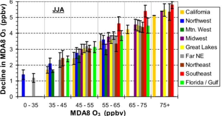
4 Impact of foreign emissions on US surface O3
Figure 6 shows the sum of the MDA8 O3 responses across
the distribution of MDA8 O3values to emissions reductions
in the three foreign source regions (EA + SA + EU, hereafter referred to as “foreign emissions”). The slight multi-model
underestimate of MDA8 O3 during spring in the Mountain
West and overestimate in the Southeast during summer are depicted as offsets between the red triangles (observations) and black squares (multi-model mean). In contrast, in the Mountain West during summer and in the Southeast dur-ing sprdur-ing, the two lines nearly lie atop one another, indi-cating very good agreement in the number of days in each bin between the multi-model mean and the observations. A comparison between the Mountain West and Southeast re-gions illustrates broad characteristics that hold true for
gen-eral East vs. West US regions (see Fig. A6 for the MDA8 O3
response in the seven other US regions), so we generalize results where applicable.
In summer, the multi-model mean over-predicts MDA8 O3
in many regions by a substantial amount (10–20 ppbv) and in
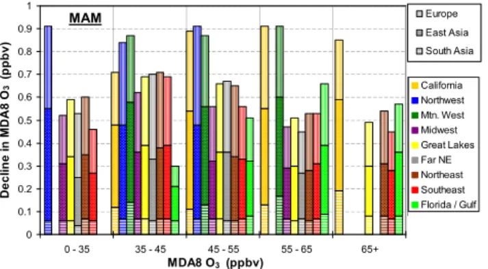
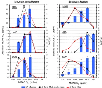
Figure 6. Number of days for each MDA8 O3 bin (right-axis) from the multi-model
mean (black squares) and observations (red triangles) and the sum of the responses of MDA8 O3 to 20% emissions reductions of anthropogenic O3-precursors (NOx + CO +
NMVOC + aerosols) in the three foreign source regions (left-axis; green columns with error bars representing 1σ of the multi-model mean) in the Mountain West (left) and Southeast (right) regions, binned by simulated MDA8 O3, for spring (MAM), summer
(JJA) and autumn (SON). Note the range of magnitudes on the y-axes. Mountain West Region
0.0 0.2 0.4 0.6 0.8 1.0 1.2 0-35 35-45 45-55 55-65 65-75 75+ MDA8 O3 (ppbv) D e c li n e i n M D A 8 O 3 (p p b v ) 0 13 26 39 52 65 78 # D a y s MAM 0 0.1 0.2 0.3 0.4 0.5 0.6 0.7 0.8 0-35 35-45 45-55 55-65 65-75 75+ MDA8 O3 (ppbv) D e c li n e i n M D A 8 O 3 (p p b v ) 0 7 14 21 28 35 42 49 56 # D a y s JJA 0.0 0.1 0.2 0.3 0.4 0.5 0.6 0.7 0.8 0-35 35-45 45-5555-65 65-75 75+ MDA8 O3 (ppbv) D e c li n e i n M D A 8 O 3 (p p b v ) 0 7 14 21 28 35 42 49 56 # D a y s SON D e c lin e i n M D A 8 O 3 (p p b v ) # D a y s 0.0 0.1 0.2 0.3 0.4 0.5 0.6 0.7 0.8 0.9 0-35 35-45 45-55 55-65 65-75 75+ MDA8 O3 (ppbv) D e c li n e i n M D A 8 O 3 (p p b v ) 0 5 10 15 20 25 30 35 40 45 # D a y s MAM 0.00 0.05 0.10 0.15 0.20 0.25 0.30 0.35 0-35 35-45 45-55 55-6565-75 75+ MDA8 O3 (ppbv) D e c li n e i n M D A 8 O 3 (p p b v ) 0 8 16 24 32 40 48 56 # D a y s JJA 0.0 0.1 0.2 0.3 0.4 0.5 0.6 0.7 0-35 35-45 45-55 55-65 65-75 75+ MDA8 O3 (ppbv) D e c li n e i n M D A 8 O 3 (p p b v ) 0 5 10 15 20 25 30 35 # D a y s SON Southeast Region D e c lin e i n M D A 8 O 3 (p p b v ) # D a y s MDA8 O3(ppbv) MDA8 O3(ppbv) MDA8 O3 (ppbv)
Foreign influence # Days_Multi-model mean # Days_Obs
Mountain West Region
0.0 0.2 0.4 0.6 0.8 1.0 1.2 0-35 35-45 45-55 55-65 65-75 75+ MDA8 O3 (ppbv) D e c li n e i n M D A 8 O 3 (p p b v ) 0 13 26 39 52 65 78 # D a y s MAM 0 0.1 0.2 0.3 0.4 0.5 0.6 0.7 0.8 0-35 35-45 45-55 55-65 65-75 75+ MDA8 O3 (ppbv) D e c li n e i n M D A 8 O 3 (p p b v ) 0 7 14 21 28 35 42 49 56 # D a y s JJA 0.0 0.1 0.2 0.3 0.4 0.5 0.6 0.7 0.8 0-35 35-45 45-5555-65 65-75 75+ MDA8 O3 (ppbv) D e c li n e i n M D A 8 O 3 (p p b v ) 0 7 14 21 28 35 42 49 56 # D a y s SON D e c lin e i n M D A 8 O 3 (p p b v ) # D a y s
Mountain West Region
0.0 0.2 0.4 0.6 0.8 1.0 1.2 0-35 35-45 45-55 55-65 65-75 75+ MDA8 O3 (ppbv) D e c li n e i n M D A 8 O 3 (p p b v ) 0 13 26 39 52 65 78 # D a y s MAM 0 0.1 0.2 0.3 0.4 0.5 0.6 0.7 0.8 0-35 35-45 45-55 55-65 65-75 75+ MDA8 O3 (ppbv) D e c li n e i n M D A 8 O 3 (p p b v ) 0 7 14 21 28 35 42 49 56 # D a y s JJA 0.0 0.1 0.2 0.3 0.4 0.5 0.6 0.7 0.8 0-35 35-45 45-5555-65 65-75 75+ MDA8 O3 (ppbv) D e c li n e i n M D A 8 O 3 (p p b v ) 0 7 14 21 28 35 42 49 56 # D a y s SON D e c lin e i n M D A 8 O 3 (p p b v ) 0.0 0.2 0.4 0.6 0.8 1.0 1.2 0-35 35-45 45-55 55-65 65-75 75+ MDA8 O3 (ppbv) D e c li n e i n M D A 8 O 3 (p p b v ) 0 13 26 39 52 65 78 # D a y s MAM 0 0.1 0.2 0.3 0.4 0.5 0.6 0.7 0.8 0-35 35-45 45-55 55-65 65-75 75+ MDA8 O3 (ppbv) D e c li n e i n M D A 8 O 3 (p p b v ) 0 7 14 21 28 35 42 49 56 # D a y s JJA 0.0 0.1 0.2 0.3 0.4 0.5 0.6 0.7 0.8 0-35 35-45 45-5555-65 65-75 75+ MDA8 O3 (ppbv) D e c li n e i n M D A 8 O 3 (p p b v ) 0 7 14 21 28 35 42 49 56 # D a y s SON D e c lin e i n M D A 8 O 3 (p p b v ) D e c lin e i n M D A 8 O 3 (p p b v ) D e c lin e i n M D A 8 O 3 (p p b v ) D e c lin e i n M D A 8 O 3 (p p b v ) D e c lin e i n M D A 8 O 3 (p p b v ) # D a y s # D a y s 0.0 0.1 0.2 0.3 0.4 0.5 0.6 0.7 0.8 0.9 0-35 35-45 45-55 55-65 65-75 75+ MDA8 O3 (ppbv) D e c li n e i n M D A 8 O 3 (p p b v ) 0 5 10 15 20 25 30 35 40 45 # D a y s MAM 0.00 0.05 0.10 0.15 0.20 0.25 0.30 0.35 0-35 35-45 45-55 55-6565-75 75+ MDA8 O3 (ppbv) D e c li n e i n M D A 8 O 3 (p p b v ) 0 8 16 24 32 40 48 56 # D a y s JJA 0.0 0.1 0.2 0.3 0.4 0.5 0.6 0.7 0-35 35-45 45-55 55-65 65-75 75+ MDA8 O3 (ppbv) D e c li n e i n M D A 8 O 3 (p p b v ) 0 5 10 15 20 25 30 35 # D a y s SON Southeast Region D e c lin e i n M D A 8 O 3 (p p b v ) # D a y s 0.0 0.1 0.2 0.3 0.4 0.5 0.6 0.7 0.8 0.9 0-35 35-45 45-55 55-65 65-75 75+ MDA8 O3 (ppbv) D e c li n e i n M D A 8 O 3 (p p b v ) 0 5 10 15 20 25 30 35 40 45 # D a y s MAM 0.00 0.05 0.10 0.15 0.20 0.25 0.30 0.35 0-35 35-45 45-55 55-6565-75 75+ MDA8 O3 (ppbv) D e c li n e i n M D A 8 O 3 (p p b v ) 0 8 16 24 32 40 48 56 # D a y s JJA 0.0 0.1 0.2 0.3 0.4 0.5 0.6 0.7 0-35 35-45 45-55 55-65 65-75 75+ MDA8 O3 (ppbv) D e c li n e i n M D A 8 O 3 (p p b v ) 0 5 10 15 20 25 30 35 # D a y s SON Southeast Region D e c lin e i n M D A 8 O 3 (p p b v ) # D a y s 0.0 0.1 0.2 0.3 0.4 0.5 0.6 0.7 0.8 0.9 0-35 35-45 45-55 55-65 65-75 75+ MDA8 O3 (ppbv) D e c li n e i n M D A 8 O 3 (p p b v ) 0 5 10 15 20 25 30 35 40 45 # D a y s MAM 0.00 0.05 0.10 0.15 0.20 0.25 0.30 0.35 0-35 35-45 45-55 55-6565-75 75+ MDA8 O3 (ppbv) D e c li n e i n M D A 8 O 3 (p p b v ) 0 8 16 24 32 40 48 56 # D a y s JJA 0.0 0.1 0.2 0.3 0.4 0.5 0.6 0.7 0-35 35-45 45-55 55-65 65-75 75+ MDA8 O3 (ppbv) D e c li n e i n M D A 8 O 3 (p p b v ) 0 5 10 15 20 25 30 35 # D a y s SON Southeast Region D e c lin e i n M D A 8 O 3 (p p b v ) # D a y s 0.0 0.1 0.2 0.3 0.4 0.5 0.6 0.7 0.8 0.9 0-35 35-45 45-55 55-65 65-75 75+ MDA8 O3 (ppbv) D e c li n e i n M D A 8 O 3 (p p b v ) 0 5 10 15 20 25 30 35 40 45 # D a y s MAM 0.00 0.05 0.10 0.15 0.20 0.25 0.30 0.35 0-35 35-45 45-55 55-6565-75 75+ MDA8 O3 (ppbv) D e c li n e i n M D A 8 O 3 (p p b v ) 0 8 16 24 32 40 48 56 # D a y s JJA 0.0 0.1 0.2 0.3 0.4 0.5 0.6 0.7 0-35 35-45 45-55 55-65 65-75 75+ MDA8 O3 (ppbv) D e c li n e i n M D A 8 O 3 (p p b v ) 0 5 10 15 20 25 30 35 # D a y s SON Southeast Region D e c lin e i n M D A 8 O 3 (p p b v ) # D a y s 0.0 0.1 0.2 0.3 0.4 0.5 0.6 0.7 0.8 0.9 0-35 35-45 45-55 55-65 65-75 75+ MDA8 O3 (ppbv) D e c li n e i n M D A 8 O 3 (p p b v ) 0 5 10 15 20 25 30 35 40 45 # D a y s MAM 0.00 0.05 0.10 0.15 0.20 0.25 0.30 0.35 0-35 35-45 45-55 55-6565-75 75+ MDA8 O3 (ppbv) D e c li n e i n M D A 8 O 3 (p p b v ) 0 8 16 24 32 40 48 56 # D a y s JJA 0.0 0.1 0.2 0.3 0.4 0.5 0.6 0.7 0-35 35-45 45-55 55-65 65-75 75+ MDA8 O3 (ppbv) D e c li n e i n M D A 8 O 3 (p p b v ) 0 5 10 15 20 25 30 35 # D a y s SON Southeast Region D e c lin e i n M D A 8 O 3 (p p b v ) D e c lin e i n M D A 8 O 3 (p p b v ) # D a y s MDA8 O3(ppbv) MDA8 O3(ppbv) MDA8 O3(ppbv) MDA8 O3 (ppbv)
Foreign influence # Days_Multi-model mean # Days_Obs
Fig. 6. Number of days for each MDA8 O3 bin (right-axis) from the multi-model mean (black squares) and observations (red triangles) and the sum of the responses of MDA8 O3 to 20% emissions reductions of anthropogenic O3-precursors (NOx+ CO + NMVOC + aerosols) in the three foreign source re-gions (left-axis; green columns with error bars representing 1σ of the multi-model mean) in the Mountain West (left) and Southeast (right) regions, binned by simulated MDA8 O3, for spring (MAM), summer (JJA) and autumn (SON). Note the range of magnitudes on the y-axes.
spring the multi-model mean under-predicts the values in the western US by a smaller amount (∼3 ppbv). We explored whether these biases were correlated with the model calcu-lated contributions from NA or foreign sources (Fig. 7a and
Figure 7. Bias in the multi-model mean vs. the modeled influence from the three foreign
source regions (SA + EA + EU; Fig. A3) during MAM in the (a) Mountain West and (b) Southeast regions. Similar plots but for the modeled NA influence during JJA are shown for the (c) Mountain West and (d) Southeast regions.
-20 -15 -10 -5 0 5 0.0 0.3 0.6 0.9 1.2 -15 -10 -5 0 5 10 15 20 0.0 0.2 0.4 0.6 0.8 1.0 Southeast Mtn. West (a) (b) r2= 0.153 r2= 0.264 B ia s i n m u lt i-m o d e l m e a n v s . o b s (p p b v )
Modeled foreign influence, SA + EA + EU (ppbv) -5 0 5 10 15 20 25 30 35 0 1 2 3 4 5 6 7 Southeast (d) -15 -10 -5 0 5 10 0 1 2 3 4 Mtn. West (c) B ia s i n m u tl i-m o d e l m e a n v s . o b s (p p b v ) Modeled NA influence (ppbv) r2= 0.070 r2= 0.017 -20 -15 -10 -5 0 5 0.0 0.3 0.6 0.9 1.2 -15 -10 -5 0 5 10 15 20 0.0 0.2 0.4 0.6 0.8 1.0 Southeast Mtn. West (a) (b) r2= 0.153 r2= 0.264 B ia s i n m u lt i-m o d e l m e a n v s . o b s (p p b v )
Modeled foreign influence, SA + EA + EU (ppbv) -5 0 5 10 15 20 25 30 35 0 1 2 3 4 5 6 7 Southeast (d) -15 -10 -5 0 5 10 0 1 2 3 4 Mtn. West (c) B ia s i n m u tl i-m o d e l m e a n v s . o b s (p p b v ) Modeled NA influence (ppbv) r2= 0.070 r2= 0.017
Fig. 7. Bias in the multi-model mean vs. the modeled influence from the three foreign source regions (SA + EA + EU; Fig. A3) dur-ing MAM in the (a) Mountain West and (b) Southeast regions. Sim-ilar plots but for the modeled NA influence during JJA are shown for the (c) Mountain West and (d) Southeast regions.
b). For spring, the negative bias shows a statistically sig-nificant relationship with the model calculated foreign con-tribution both in the western US and the Southeast region. This relationship holds true for most regions of the country (Fig. A7). For summer, the multi-model mean shows essen-tially no relationship between the positive bias and model calculated NA contribution. These results suggest that the multi-model mean may be under-predicting the foreign con-tribution, however other factors that vary in the same way could also explain this result. In contrast, the lack of a rela-tionship between the summer bias and the domestic contri-bution (Fig. 7c and d) argues that the bias is present in nearly all airmasses (bias ranges from −2 to +30 ppbv), regardless
of the degree of local O3buildup.
4.1 Seasonal and regional differences in the influence
from foreign emissions
Figure 6 reveals the well-documented peak in foreign
influ-ence on surface O3 in the western US during spring (e.g.,
Holzer et al., 2005; Liang et al., 2004; Wang et al., 2006),
and we show here that foreign influence on surface O3in the
eastern US also peaks in spring. Each individual model sim-ulated this change in seasonal influences. In the western US, a 20% anthropogenic emissions reduction in the three NH
foreign source regions decreases MDA8 O3by ∼0.9 ppbv in
spring. In contrast, the response of MDA8 O3 in the
east-ern US to the same emissions reductions in spring is ap-proximately 50% less at ∼0.55 ppbv. In the western US, the summed response to foreign emissions reductions of 20% is ∼0.5 ppbv in summer and ∼0.6 ppbv in autumn. Simi-lar values for the eastern US are ∼0.2 ppbv in summer and ∼0.4 ppbv in autumn.
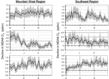
Figure 8. Multi-model mean (black line) and 1σ of the multi-model mean (gray shading)
in the day-to-day variability of the sum of the responses of MDA8 O3 to 20% emissions
reductions in anthropogenic O3−precursors (NOx + CO + NMVOC + aerosols) in the
three foreign sources regions (SA + EA + EU; Fig. A3) for the Mountain West (left) and Southeast regions (right). Note the range of magnitudes on the y-axes.
0.0 0.2 0.4 0.6 0.8 1.0 1.2 J J A D e c li n e i n M D A 8 O 3 (p p b v ) 0.0 0.2 0.4 0.6 0.8 1.0 S O N D e c li n e i n M D A 8 O 3 (p p b v ) 0.0 0.3 0.6 0.9 1.2 1.5 M A M D e c li n e i n M D A 8 O 3 (p p b v ) 0.0 0.2 0.4 0.6 0.8 1.0 1.2 M A M D e c li n e i n M D A 8 O 3 (p p b v ) -0.2 0 0.2 0.4 0.6 J J A D e c li n e i n M D A 8 O 3 (p p b v ) -0.3 -0.1 0.1 0.3 0.5 0.7 0.9 S O N D e c li n e i n M D A 8 O 3 (p p b v )
Mountain West Region Southeast Region
D e c lin e i n M D A 8 O 3 (p p b v ) D e c lin e i n M D A 8 O 3 (p p b v ) 0.0 0.2 0.4 0.6 0.8 1.0 1.2 J J A D e c li n e i n M D A 8 O 3 (p p b v ) 0.0 0.2 0.4 0.6 0.8 1.0 S O N D e c li n e i n M D A 8 O 3 (p p b v ) 0.0 0.3 0.6 0.9 1.2 1.5 M A M D e c li n e i n M D A 8 O 3 (p p b v ) 0.0 0.2 0.4 0.6 0.8 1.0 1.2 M A M D e c li n e i n M D A 8 O 3 (p p b v ) -0.2 0 0.2 0.4 0.6 J J A D e c li n e i n M D A 8 O 3 (p p b v ) -0.3 -0.1 0.1 0.3 0.5 0.7 0.9 S O N D e c li n e i n M D A 8 O 3 (p p b v )
Mountain West Region Southeast Region
D e c lin e i n M D A 8 O 3 (p p b v ) D e c lin e i n M D A 8 O 3 (p p b v ) D e c lin e i n M D A 8 O 3 (p p b v ) D e c lin e i n M D A 8 O 3 (p p b v ) D e c lin e i n M D A 8 O 3 (p p b v ) D e c lin e i n M D A 8 O 3 (p p b v ) D e c lin e i n M D A 8 O 3 (p p b v ) D e c lin e i n M D A 8 O 3 (p p b v ) D e c lin e i n M D A 8 O 3 (p p b v ) D e c lin e i n M D A 8 O 3 (p p b v ) D e c lin e i n M D A 8 O 3 (p p b v )
Fig. 8. Multi-model mean (black line) and 1σ of the multi-model mean (gray shading) in the day-to-day variability of the sum of the responses of MDA8 O3 to 20% emissions reductions in an-thropogenic O3-precursors (NOx+ CO + NMVOC + aerosols) in the three foreign sources regions (SA + EA + EU; Fig. A3) for the Mountain West (left) and Southeast regions (right). Note the range of magnitudes on the y-axes.
In Fig. 8 we show the multi-model mean (black line)
±1σ (gray shading) summed MDA8 O3response to the
for-eign emissions reductions of 20% at daily resolution for the Mountain West and Southeast regions (Fig. A8 shows the re-sults for the other seven regions). Note that in contrast to Fig. 5, there is no way to use observations to directly confirm the results presented in Fig. 8. The season of greatest inter-continental influence (spring) is also the season of greatest inter-model spread in the foreign influence, both in absolute
(σ ) and relative (σr,m) terms. An annual cycle in the
magni-tude of the foreign impact on MDA8 O3 can be seen in all
regions, peaking in spring, declining by over 50% in summer and increasing slightly in autumn to return to values that are
∼33% below the maximum influence in spring. It is worth
noting that no model predicts a foreign influence on the order
of tens of ppbv of O3that have been reported through
obser-vational studies (Yienger et al., 2000; Kotchenruther et al., 2001; Hudman et al., 2004; Jaffe et al., 2004; Weiss-Penzias et al., 2004; Keating et al., 2005). If we linearly scale even
the strongest model surface O3response to 100% emissions
reduction in the three foreign source regions, the maximum event in the western US during spring has a summed for-eign contribution of ∼9 ppbv (∼2 ppbv from SA; ∼4 ppbv from EA; ∼3 ppbv from EU). However, these observational studies are not directly comparable to the multi-model results presented here for several reasons: (1) most of these observa-tional studies are free tropospheric/elevated aircraft studies,
whereas we focus on surface O3, (2) the observational
stud-ies often focus on foreign influence within a plume, whereas the multi-model results have been averaged over a large spa-tial area, and (3) observational studies typically attribute