HAL Id: hal-01342843
https://hal.univ-lorraine.fr/hal-01342843
Submitted on 6 Jul 2016HAL is a multi-disciplinary open access
archive for the deposit and dissemination of sci-entific research documents, whether they are pub-lished or not. The documents may come from teaching and research institutions in France or abroad, or from public or private research centers.
L’archive ouverte pluridisciplinaire HAL, est destinée au dépôt et à la diffusion de documents scientifiques de niveau recherche, publiés ou non, émanant des établissements d’enseignement et de recherche français ou étrangers, des laboratoires publics ou privés.
networks using Horton parameters and A*. Application
to a synthetic case
Pauline Collon-Drouaillet, Vincent Henrion, Jeanne Pellerin
To cite this version:
Pauline Collon-Drouaillet, Vincent Henrion, Jeanne Pellerin. An algorithm for 3D simulation of branchwork karst networks using Horton parameters and A*. Application to a synthetic case. Geo-logical Society Special Publication, 2012, 370 (1), pp.295-306. �10.1144/SP370.3�. �hal-01342843�
Collon-Drouaillet P., Henrion V., Pellerin J. (2012). An algorithm for 3D simulation of branchwork karst networks using Horton parameters and A* Application to a synthetic case. Geological Society, London, Special Publications, 370(1), 295–306. DOI: 10.1144/SP370.3
An algorithm for 3D simulation of branchwork karst networks using Horton
parameters and A?. Application to a synthetic case.
Pauline Collon-Drouaillet1*, Vincent Henrion1,2 & Jeanne Pellerin1 June 2011
1 CRPG-CNRS, ENSG, Universit´e de Lorraine, rue du doyen Marcel Roubault, BP 40, 54501
Vandoeuvre-l`es-Nancy, France.
∗Corresponding author (e-mail: pauline.collon@ensg.inpl-nancy.fr ; tel: (+33)3 83 59 64 20) 2 Now at: Total EP, CSTJF, avenue Larribau, Pau, France.
Abstract
This paper presents a method to stochastically simulate 3D karstic networks and more specif-ically branchwork pattern cave systems. Considering that they can be compared to 3D fluvial networks, the topological classification of Strahler and the corresponding ratios of Horton are used to define three morphometric parameters. These parameters are integrated in an algorithm which computes branches hierarchically to obtain a final network organised around the main observed inlet and outlet with a branching complexity controlled by the user. Each branch corresponds to a low-cost path between two points calculated with the A? graph search algorithm. Speleogenetic information on inception horizons, palaeo-water tables and fractures is accounted for by adapted definitions of the searching functions of A?. The method is demonstrated on a 3D synthetic case with discrete fractures networks, inception horizons and a palaeo-water table. The simulated karsts have a realistic geometry and are geologically consistent.
Simulation of 3D karstic networks is often required to build consistent geomodels in carbonate reser-voir environments for various applications: water supply management, complex carbonate petroleum reservoirs studies, civil ingeneering, etc. Genetic approaches try to reproduce the physical processes leading to karst formation (Dreybrodt et al., 2005; Ford & Williams, 2007). Because of their extreme computational heaviness, they are essentially operating in 2D (e.g. Kaufman & Braun, 2000; Kaufman & Romanov, 2008). Moreover they are based on various parameters (e.g. palaeo-climate, boundary conditions, etc.) that are not always available (Dreybrodt & Gabrovsek, 2003).
Static approaches directly simulate the result of the karstification process but to our knowledge only a few attempts have been made in this direction. Jaquet et al. (2004) used a modified lattice-gas automaton for the discrete simulation of karstic networks. As it uses a random-walk technique, this method would be difficult to constrain exactly with field data. Karst networks are computed independently in several 2D horizontal layers and the addition of vertical conduits where karst were observed at surface provides a 2.5D image. The orientation of the lattice has a significant impact on the results since its segments determine the distribution of faults and fractures considered and imposed their orthogonal orientations. The different approach of Labourdette et al. (2007) focuses
on flank-margin caves modelling with an object-based method. Providing realistic geometries and volumes with a limited number of parameters, the main drawback of this method is that it needs a 3D model of surveyed caves. Indeed, it relies on an iterative procedure that stops when differences in volume and shape between simulated and observed caves become small enough. It also uses a dissolution probability cube based on hypothesis specific to flank margin caves. Particularly adapted in the case of flank-margin caves, the method is not directly applicable to other karst types. Moreover, none of these two methods considers the global shape of the networks.
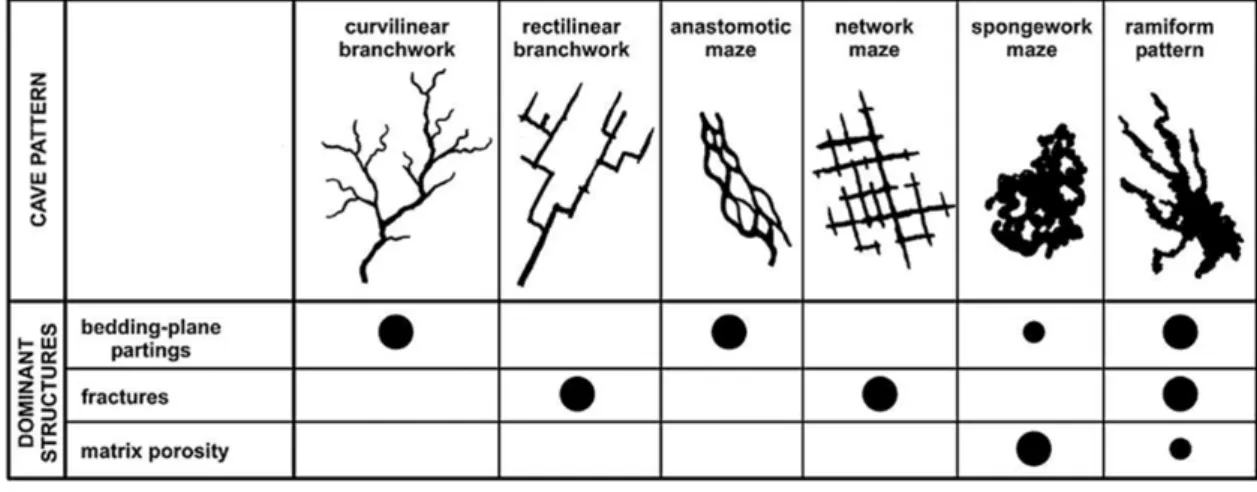
According to Palmer (2003) karst patterns can be qualitatively separated in three main families related to speleogenetical context (Fig. 1): i) branchwork patterns (curvilinear or rectilinear); ii) maze patterns (anastomotic, network, spongework); and iii) ramiform patterns. In this article, we focus on branchwork karsts and present a method to constrain their simulation by specific parameters.
Figure 1: Cave pattern classification after Palmer (2003): ”Common patterns of solutional caves. Dot sizes show the relative abundance of cave types in each of the listed categories.
Single-passage caves are rudimentary or fragmentary versions of those shown here.”
The global workflow, first introduced by Henrion et al. (2007), consists in four main steps described in the first section. The basic idea is to compute a skeleton of the karstic network and to simulate stochastically the karst envelope around it. The specific algorithm developed to build branchwork skeletons with a control on the branching complexity is presented in the second section. It is based on a hierachical computation of elementary branches, each branch being the lowest-cost path between two points computed with the A? graph search algorithm. The searching functions of A? are defined to account for speleogenetic information. The last section, which can be read independantly, demonstrates the method on a 3D synthetic case with inception horizons and fractures showing the potential of the approach.
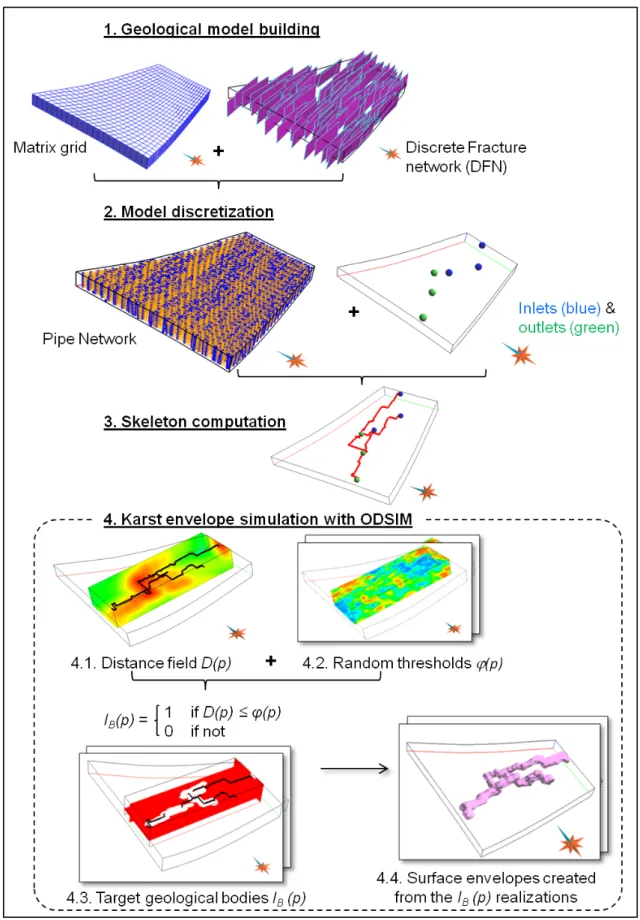
General workflow for karst simulation
Fig. 2 summarizes the four main steps of the global workflow.
Geological model building. The capacity of the geomodel to synthesize geological data and knowl-edge of the studied zone impacts the complete workflow: surfaces that favour karstogenesis have to be integrated at this step. Following basic principles of 3D geomodelling (Caumon et al., 2009) ensures the consistency of the model. The petrophysical properties, permeability and porosity, can be defined indifferently with kriging or sequential gaussian simulation (e.g. Goovaerts (1997)). Discrete Fracture Networks can be simulated with the stochastic method developed by Mac´e (2006).
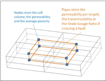
Discretization of the geomodel into a graph of connectivities. The graph used here is a PipeNetwork: an unstructured connectivity graph designed to perform flow simulations (Vitel, 2007). It consists in a set of pipes connecting a set of nodes, which respectively correspond to the facets of the control volumes
Figure 2: General workflow for stochastic 3D karst simulation
and the grid points of a reservoir simulation grid. From a geometrical point of view, it corresponds to the partial topological dual of a corner-point grid (Fig. 3). The PipeNetwork provides a unified structure for various types of geomodels: structured grids combined or not with fracture networks
or unstructured grids with faults and horizons. Various properties simulated in the geomodel can be transferred on the graph (e.g. permeability) and some other may be computed during the discretization process (e.g. volumes). A specificity of the PipeNetwork is to store the properties of the media on nodes (e.g. permeability, volume), while properties concerning flow transmission are stored on pipes (e.g. transmissibility, permeability per length). Inlets and outlets can be imposed by field observation or stochastically simulated.
Figure 3: PipeNetwork as partial topological dual of a block-centered corner-point grid (Blue cubes: nodes, orange lines: pipes) (modified from Vitel (2007))
Karst skeleton computation. The skeleton of the karst is extracted from the previous graph as preferential flow paths between inlets and oulets points. This step controls the high scale geometry of the karst. Thus, it is the key part for a process dedicated to the modeling of branchwork patterns and it is fully detailed in the next section of this paper.
Computation of realistic 3D karst envelopes. This final step relies on the object-distance simulation method (ODSIM ) proposed by Henrion et al. (2010). It computes for each point p = [px py pz]T of a
grid G the Euclidean distance to a geological body skeleton providing a 3D distance field D(p) (Fig. 2, 4.1). This distance field is then truncated by a spatially correlated random threshold ϕ (p) which may be generated using Sequential Gaussian Simulation or other stochastic simulation method (e.g. Goovaerts, 1997; Deutsch & Journel, 1997) (Fig. 2, 4.2). The resulting object is identified in the grid by a binary categorical property IB (Fig. 2, 4.3) defined by
IB(p) =
(
1 if D(p) ≤ ϕ(p)
0 if not (1)
During this process, the extension of karst conduits is controlled by the distribution (PDF) of the threshold while the parameters of the variogram control the roughness and anistropy of karst conduits. Indeed, higher variogram ranges involve lower changes of the threshold values, providing a smoother enveloppe. If the ranges vary with the directions, this will be reflected in the geometrical evolution of karst conduits that will be smoother along the mean directions. An iterative Gibbs sampler (Geman & Geman, 1984) with inequality constraints allows to condition the threshold simulation to well data while preserving its spatial structure and histogram (Henrion et al., 2010).
Methodology for branchwork karst pattern generation
An algorithm to control the branching complexity of karst networks
Branchwork patterns have a typical topology, characterized by a hierarchical organization excluding cycles (only one path between two points) . A solution to reproduce this hierarchy is to extract a main
path, and compute secondary paths connected to it (Bonneau et al., 2010). But none of the previously developed techniques integrates a possibility to control the branching complexity of the networks.
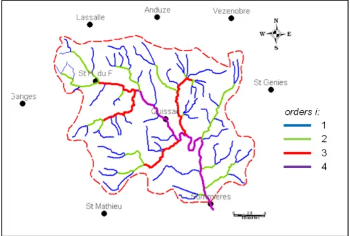
Developed for hydrological applications, the topological classification of Strahler (1952) can be applied on any directed graph tree. Each segment of the tree is assigned an order i with the followings rules (Fig. 4):
• each segment with no parent (i.e. with no affluent for a stream) has an order equal to 1;
• a segment formed from the confluence of two segments of order i, has an order equal to i + 1;
• a segment formed from the confluence of two segments of order m and n, has an order equal to max(m, n).
The Horton-Strahler number of a tree is defined as the order of its outlet. It is denoted Ko in this
work.
Figure 4: Example of Strahler classification on a hydrological network (South France) where the Horton-Strahler number is equal to 4
The branching complexity of a network can be described by the Horton bifurcation ratio RB, based
on the law of stream numbers (Horton, 1945) which states that the ratio NKi NKi+1
where NKi is the
number of paths of order i, converges to a constant when order increases. Moreover, the Horton law of stream lengths states that a geometric relationship exists between the cumulated length of streams of a given order Li and the corresponding order i, i.e. the ratio
Li
Li+1
converges to a constant called the Length Ratio RL.
From a geometrical point of view, a branchwork pattern is an oriented graph tree. So, Strahler classification can be applied to it. The geostatistical and fractal studies of length caves made by Curl (1986) demonstrate that the lengths of caves in a given region and the size of modular elements constituting them are distributed hyperbolically. This indicates that a self-similarity appears in these complex systems. Despite the fact that Horton laws on stream numbers and stream lengths have not been proved for karstic systems, the Horton ratios may help to reproduce this self-similarity. Thus, the three parameters, Ko, RB and RL, are integrated in a new algorithm to simulate branchwork karsts
controlled by the user.
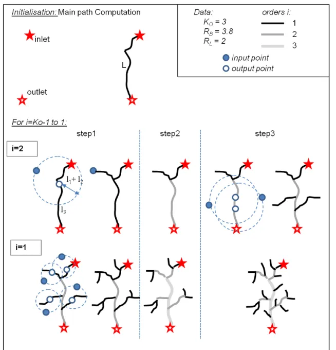
The algorithm (Fig. 5) first computes a main path between the given input and output. Then, for each order i from (Ko− 1) to 1, the following three steps are performed:
Figure 5: The different steps of the branchwork network algorithm. The initialisation consists in the extraction of a main path linking inlet and outlet. Then, for each order i from (Ko− 1)
to 1, the step 1 computes 1 path connected to each path of order 1, the second step updates Horton orders and the third step generates the remaining paths on segments of order > 1 to honour the bifurcation ratio RB. The input points definition in step 1 and 3 and the output
points choice in step 1 are guided by the values of the length ratio RB
1. Compute 1 path connected to each path of order 1 to increase its order. This is done using a length smooth constraint described below.
2. Update Horton orders;
3. Generate the (NKi− 2NKi+1) remaining paths with output points randomly chosen on paths of
order > 1 guaranteeing that Horton orders i are preserved.
The length smooth constraint enforces the use of the RLratio. Considering li as the average length
have the following equations: Li= Ni× li L = Ko P i=1 li (2) Thus: li li+1 = RL RB = r (3)
which leads to:
li = rKo−i× lKo (4) and: lKo= L Ko−1 P j=0 rj (5)
To perform the first step of the previous algorithm for a current order i, we impose the output point pouti of the new path to be located at a distance li+1 from the downstream segment extremity. Then,
the new input point pini is randomly chosen on the half upper sphere of radius l = rand[0.5;1]∗
i−1
P
j=1
lj
where rand[0.5;1]is a random number chosen between 0.5 and 1. As karsts form from surface infiltration,
the input point is vertically projected on the upper part of the PipeNetwork. The new pair of points [pini; pouti] is then used to compute the connected path. The third step is quite similar of the first one,
except that the output point is randomly chosen on an existing path of order 1. As the computed paths between two points are not straight lines (see the detailed method below) and as the path extraction ends when crossing an existing segment, the length of the resulting path is different from the used radius l (often superior to l, explaining the use of the random multiplier).
Thus, the RLratio guides the simulation but is not strictly honoured justifying the notion of smooth
constraint. The RB ratio is more constraining but the use of non-integers permit to obtain network
with different values. On the contrary, the Horton-Strahler number Ko is always strictly respected
and can be considered as a hard constraint.
Using A? for single path computation
A? algorithm allows to easily compute single karst branches honouring given input and output points. These points might be actual inlet and/or outlet of the network or location computing by the branch-work karst simulation algorithm described in the previous section. A? is a graph search algorithm that aims at finding the least cost path between two given nodes (Hart et al., 1968). It uses a best-first search, i.e. it first explores the most promising node chosen according to a specified rule, and derives from Edsger Dijkstra’s 1959 algorithm (Dijkstra, 1959). A better performance (with respect to time) is obtained thanks to the use of a heuristic function f (x). f is the sum of (1) a cost function g(x), which is the cumulated cost from the starting node to the current node, and (2) an admissible heuristic estimate h(x) of the distance to the goal. Two rules have to be respected:
• The cost has to be strictly positive: g(x) > 0;
• The heuristic estimate has to be admissible, i.e. it must not overestimate the distance to the goal: h(x) < g(x, goal), where g(x, goal) is the minimal cost from x to goal.
To use A? for karst skeleton computation, these two functions must be defined consistently. Despite the complexity of the phenomenons involved, speleologists agree that knowing two connected points, karstic conduits develop preferentially along paths with high hydraulic conductivity and short length (Ford & Williams, 2007, chap. 7). Thus, we define the cost on a pipe as a function of the inverse of the permeability per length KLij (Eq. 6). The permeability per length is a weighted average permeability
and divided by the pipe length (Eq. 7). The resulting cost, proportional to 1 KLij
, is homogeneous to a time and thus it can be summed and is independent of mesh resolution.
costij = 1 KLij × gravij (6) KLij = 1 dij × ki× voli+ kj× volj voli+ volj (7) with:
• ki the permeability at point i;
• voli the volume of the cell represented by node i;
• dij the distance between the points i and j.
The gravity gravij is included in the cost computation has a multiplier coefficient (Eq. 6) to avoid
vertically oscillating paths (Eq. 8)
gravij = 1 if 4zij ≥ 0 1 −4zij dij if 4zij < 0 (8)
The admissible heuristic is a function of the distance from the current node to the output node (Eq. 9). Unit homogeneity and A? requirements are guaranteed by the use of a multiplier coefficient equal to the maximal cost M cp encountered on the PipeNetwork multiplied by the length of this maximal cost pipe Lmp (Eq. 9):
heurj =
dj,output
max (KL× d)
(9)
where dj,output is the distance between the point j and the output.
With these definitions of the cost and the heuristic, the A? algorithm extracts paths between two points of a PipeNetwork using hydraulic conductivity information. Speleogenetical concepts and geological information might be included at the geomodel building step and will then be taken into account when the skeleton is computed. Different kind of surfaces have been identified as preferential surfaces for karst development: inception horizons are the restricted numbers of bedding planes within the limestone series along which a karstic network tends to develop (Lowe, 1992), palaeo-water tables and fractures are also proved to favour karst development (Dreybrodt & Gabrovsek, 2003). For incep-tion horizons and palaeo-water table, an adapted building of the geomodel using a grid conformable to the considered surfaces with a local mesh refinement along these levels allows their integration in the PipeNetwork. Giving these surfaces higher values of hydraulic conductivity promotes the simulation of paths along them. The object-based method developed by Mac´e (2006) stochastically simulates a discrete fracture networks (DFN) from data on their orientation, extension and density. These frac-tures can be jointly discretized with the geomodel (Vitel, 2007) allowing to generate karst skeletons strongly influenced by their presence.
Application on a synthetic case
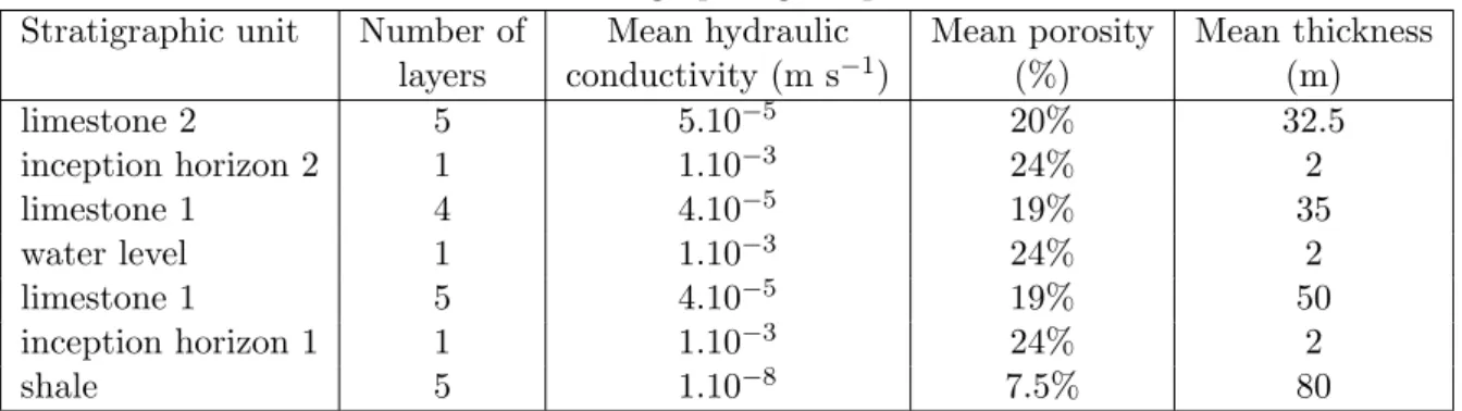
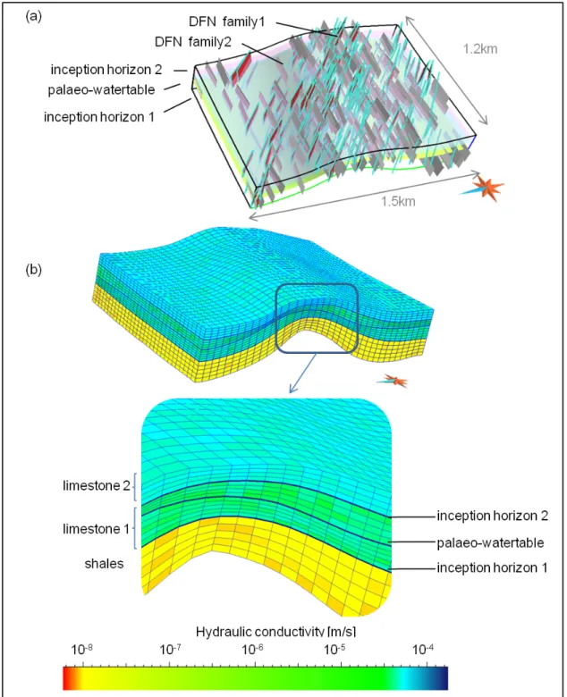
The method is applied on a 3D synthetic case. The fractured geological system is made of a succession of three stratigraphic units, from base to top: one layer of shale overhanged by two layers of limestone. Two inception horizons separate these units and a palaeo-water table is located inside the bottom limestone unit (Fig. 6a). Two fracture families are considered. All these surfaces favour karstogenesis. A stratigraphic grid (cell numbers: 30 × 37 × 21) is built from these data, with thinner cells (2m high) centered on the inception horizons and the palaeo-water table (Fig. 6b). The hydraulic conductivities and porosities of the different units (Table 1) are simulated using an unconditional
sequential gaussian simulation (Goovaerts, 1997) with a uniform law and a spherical variogram (with ranges : 200m, 200m and 50m). The two Discrete Fracture Networks (DFN) are simulated (Fig. 6a) according to the workflow proposed by Mac´e et al. (2004), with a higher density of fracturation along the fold axis. Their properties, following triangular laws, are indicated in Table 2.
Table 1: Stratigraphic grid specifications
Stratigraphic unit Number of Mean hydraulic Mean porosity Mean thickness
layers conductivity (m s−1) (%) (m) limestone 2 5 5.10−5 20% 32.5 inception horizon 2 1 1.10−3 24% 2 limestone 1 4 4.10−5 19% 35 water level 1 1.10−3 24% 2 limestone 1 5 4.10−5 19% 50 inception horizon 1 1 1.10−3 24% 2 shale 5 1.10−8 7.5% 80
Table 2: Discrete Fracture Networks properties
DFN Hydraulic aperture Dip(o) Dir (o) Length (m) Width(m)
cond. (m s−1) (m) min-mode-max min-mode-max min-mode-max min-mode-max
1 1.2 10−3 0.003 85-90-100 85-90-100 150-210-250 70-100-120
Figure 6: 3D Geological synthetic model of the area in which karstic network is generated: (a) The three surfaces favouring karstogenesis and the two discrete fracture networks; (b) The
corresponding stratigraphic grid with simulated hydraulic property values.
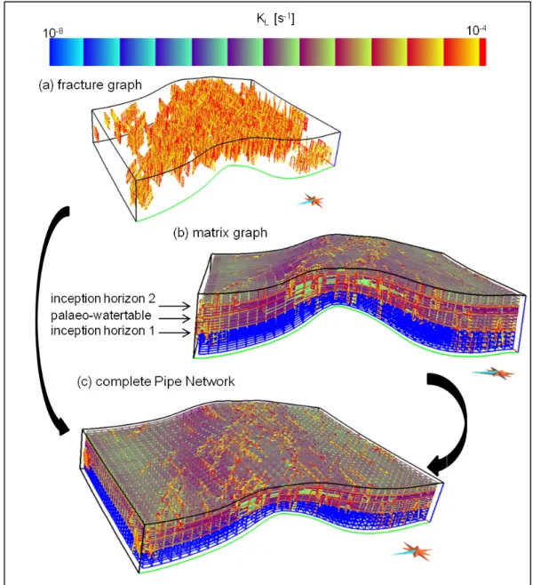
The model is discretized into a PipeNetwork composed of 50605 nodes, including 27300 nodes for the fractures (Fig. 7). The permeability per length values range from 1.7 10−11s−1 in belower shale to around 10−2s−1 in short pipes of fractures, inception horizons and palaeo-water table.
Figure 7: PipeNetwork resulting from the joined discretization of the stratigraphic grid and the two DFN (c). Preferential surfaces for karst development, (a) fractures , (b)inception horizons and palaeo-water table have a higher permeability per length (orange) than the layers.
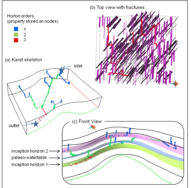
A network simulation is performed between inlet and outlet (Fig. 8) with the following values: Ko= 3, RB = 2.8 and RL= 3.5. The obtained branchwork skeleton honours its input parameters Ko
and RB and the skeleton paths are located preferentially along the fractures, the inception horizons
Figure 8: Branchwork skeleton obtained with Ko = 3, RB = 2.8 and RL = 3.5 and given
inlet and outlet. (a) The branching connectivity respects the input parameters; (b) Top view: the skeleton paths are located preferentially along the fractures; (c) Vertical cross-section: the paths are also preferentially located around the inception horizons and the water table due to
their higher permeability.
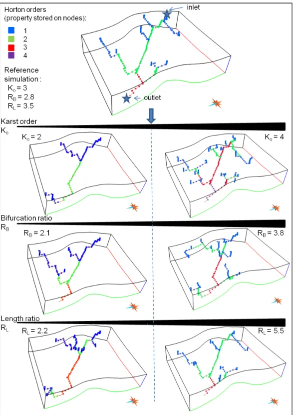
To illustrate the influence of the three morphometric parameters several simulations have been performed, each time with the same random seed for the search of input points (Fig. 9). Consistently with their definitions, the Kovalue controls the hierarchical organisation i.e. the branching complexity
of the network, and imposes an order to the outlet of the karst. Increasing the bifurcation ratio RB
produces denser networks without changing the global order, i.e. for the same Ko value it generates
Figure 9: Branchwork skeletons obtained by changing the values of the three morphometric parameters Ko, RB and RL. (a) The Ko value controls the hierarchical organisation i.e. the
branching complexity; (b) The global number of paths is increasing with the RB parameter;
(c) An higher value of RL involves higher lengths of secondary paths.
As presented in the global workflow, the object-distance simulation method (ODSIM ) can be applied on the resulted skeletons to generate stochatically several 3D envelopes of the network (Henrion et al., 2010). The Fig. 10 illustrates this method on the reference skeleton computed on the synthetic case. In karstic systems the geometry of the voids is perceptible at a local scale (dimensions from meters to ten or so meters) whereas the previous studied skeletons was computed at a regional scale (kilometer
or so). The thresholds have been simulated using a triangular distribution (PDF) (minimum = 1 , mode = 2, maximum = 15) and a gaussian variogram with an azimuth = 60, a dip = 0, ranges = [30 25 15], no nugget effect and a cumulative sill = 1. The distance field has been then truncated by these thresholds to produce three binary categorical properties. To make easiest the visualization of the results, envelope surfaces have been extracted from grid isovalues.
Conclusions and perpectives
The developed methodology generates branchwork karstic networks with a user control on branching complexity and gives promising results. However, the choice of using Horton-Strahler parameters could be discussed. Indeed these parameters have been proven relevant in the case of fluvial networks but not yet in the case of natural karstic systems. The main differences are that karst are not organised along a unique horizon, that often some multiple interconnections appear, etc. A preliminary work is going on to test the relevancy of the Strahler orders on natural karsts. The few multiple interconnections could be reproduced by additional path computations. However, a step of formalism and automation is required to obtain an effective tool.
Further work will aim at providing tools to simulate the other karst patterns. The network maze is quite easy to simulate by the direct application of the ODSIM method on an adequate selection of DFN fractures but improvements can be done considering their automation and calibration by the user. Anastomotic mazes, spongework mazes and ramiform patterns require specific developments to be deliberately simulated.
Regarding the karst envelope, the ODSIM method generates various shapes but could still be improved to integrate field data like seismic information, a library of natural karstic shapes and their geological environment.
We would like to thank the industrial and academic members of the Gocad Consortium, ASGA, for their support, Paradigm Geophysical for providing the Gocad Software and API, and the French National Scientific Research Center CNRS-CRPG for their support.
References
Bonneau, F., Henrion, V. & Collon-Drouaillet, P., 2010. Genetic-like modeling of karst net-work. In Proc. 30th Gocad Meeting, Nancy, France.
Caumon, G., Collon-Drouaillet, P., Le Carlier de Veslud, C., Viseur, S. & Sausse, J., 2009. Surface-based 3d modeling of geological structures. Mathematical Geosciences, 41, 927–945.
Curl, L. R., 1986. Fractal dimensions and geometries of caves. Mathematical Geology, 18, 765–783.
Deutsch, C. V. & Journel, A. G., 1997. GSLIB: Geostatistical Software Library and User’s Guide (Applied Geostatistics). Oxford University Press, USA.
Dijkstra, E. W., 1959. A note on two problems in connexion with graphs. Numerische Mathematik, 1, 269–271, doi:10.1007/BF01386390.
Dreybrodt, W., Gabrovek, F. & Romanov, D., 2005. Processes of speleogenesis: a modeling approach. Karst Research Institut - ZRC.
Dreybrodt, W. & Gabrovsek, F., 2003. Basic processes and mechanisms governing the evolution of karst. Speleogenesis and Evolution of Karst Aquifers, The Virtual Scientific Journal, 1, 26.
Ford, D. & Williams, P., 2007. Karst Hydrogeology and Geomorphology. John Wiley and Sons, Ltd.
Geman, S. & Geman, D., 1984. Stochastic relaxation, gibbs distribution and the bayesian restoration of images. IEEE Trans Pattern Anal Mach Intell, 6(6), 721–741.
Goovaerts, P., 1997. Geostatistics for natural resources evaluation. Applied Geostatistics, Oxford University Press, New York, NY, 483p.
Hart, P. E., Nilsson, N. J. & Raphael, B., 1968. A formal basis for the heuristic determination of minimum cost paths in graphs. IEEE Trans. Syst. Sci. and Cybernetics, SSC-4, 100–107.
Henrion, V., Caumon, G. & Cherpeau, N., 2010. Odsim: An object-distance simulation method for conditioning complex natural structures. Mathematical Geosciences, 42(8), 911–924.
Henrion, V., Caumon, G., Vitel, S. & Kedzierski, P., 2007. Stochastic simulation of cave systems in reservoir modeling. In Proc. 27th Gocad Meeting, Nancy, France, 11.
Horton, R. E., 1945. Erosional development of streams and their drainage basins; hydrophysical approach to quantitative morphology. Bulletin Geological Society of America, 56, 275–370.
Jaquet, O., Siegel, P., Klubertanz, G. & Benabderrhamane, H., 2004. Stochastic discrete model of karstic networks. Advances in Water Resources, 27, 751–760.
Kaufman, G. & Braun, J., 2000. Karst aquifer evolution in fractured, porous rocks. Water Resources Research, 36(6), 1381–1391.
Kaufman, G. & Romanov, D., 2008. Cave development in the swabian alb, south-west germany: A numerical perspective. Journal of Hydrology, 349, 302–317.
Labourdette, R., Lascu, I., Mylroie, J. & Roth, M., 2007. Process-like modeling of flank-magin caves: from genesis to burial evolution. Journal of Sedimentary Research, 77, 965–979.
Lowe, D., 1992. The origin of limestone caverns: an inception horizon hypothesis. Ph.D. thesis, Manchester Polytechnic, United Kingdom.
Mac´e, L., 2006. Caract´erisation et mod´elisation num´erique tridimensionnelle des r´eseaux de fractures naturelles. Ph.D. thesis, INPL, Nancy, France.
Mac´e, L., Souche, L. & Mallet, J.-L., 2004. 3d fratures characterization based on geomechanics and geologic data uncertainties. In Proc. 24th Gocad Meeting, Nancy, France.
Palmer, A. N., 2003. Speleogenesis in carbonate rocks. Speleogenesis and Evolution of Karst Aquifer, The virtual Scientific Journal, 1, 11.
Strahler, A., 1952. Hypsometric (area-altitude) analysis of erosional topography. Bulletin Geological Society of America, 63, 1117–1142.
Vitel, S., 2007. M´ethodes de discr´etisation et de changement d’ ´echelle pour les r´eservoirs fractur´es 3D. Ph.D. thesis, INPL, Nancy, France.