HAL Id: hal-03148693
https://hal.archives-ouvertes.fr/hal-03148693
Submitted on 28 Feb 2021
HAL is a multi-disciplinary open access
archive for the deposit and dissemination of
sci-entific research documents, whether they are
pub-lished or not. The documents may come from
teaching and research institutions in France or
abroad, or from public or private research centers.
L’archive ouverte pluridisciplinaire HAL, est
destinée au dépôt et à la diffusion de documents
scientifiques de niveau recherche, publiés ou non,
émanant des établissements d’enseignement et de
recherche français ou étrangers, des laboratoires
publics ou privés.
AGN black hole mass estimates using polarization in
broad emission lines
D. Savić, R. Goosmann, L. Č. Popović, F. Marin, V. Afanasiev
To cite this version:
D. Savić, R. Goosmann, L. Č. Popović, F. Marin, V. Afanasiev. AGN black hole mass estimates using
polarization in broad emission lines. Astronomy and Astrophysics - A&A, EDP Sciences, 2018, 614,
pp.A120. �10.1051/0004-6361/201732220�. �hal-03148693�
https://doi.org/10.1051/0004-6361/201732220 c ESO 2018
Astronomy
&
Astrophysics
AGN black hole mass estimates using polarization in broad
emission lines
-D. Savi´c
1,2,4, R. Goosmann
1, L. ˇ
C. Popovi´c
2,3, F. Marin
1, and V. L. Afanasiev
11 Observatoire Astronomique de Strasbourg, Université de Strasbourg, CNRS, UMR 7550, 11 rue de l’Université, 67000 Strasbourg,
France
2 Astronomical Observatory Belgrade, Volgina 7, 11060 Belgrade, Serbia
e-mail: [email protected]
3 Department of Astronomy, Faculty of Mathematics, University of Belgrade, Studentski trg 16, 11000 Belgrade, Serbia 4 Astrophysical Observatory of the Russian Academy of Sciences, Nizhnij Arkhyz, Karachaevo-Cherkesia 369167, Russia
Received 1 November 2017/ Accepted 6 January 2018
ABSTRACT
Context.The innermost regions in active galactic nuclei (AGNs) have not yet been spatially resolved, but spectropolarimetry can provide insight into their hidden physics and geometry. From spectropolarimetric observations in broad emission lines and assuming equatorial scattering as a dominant polarization mechanism, it is possible to estimate the mass of supermassive black holes (SMBHs) residing at the center of AGNs.
Aims.We explore the possibilities and limits, and put constraints on the method for determining SMBH masses using polarization in broad emission lines by providing more in-depth theoretical modeling.
Methods.We used the Monte Carlo radiative transfer code stokes to explore polarization properties of Type-1 AGNs. We modeled equatorial scattering using flared-disk geometry for a set of different SMBH masses assuming Thomson scattering. In addition to the Keplerian motion, which is assumed to be dominant in the broad-line region (BLR), we also considered cases of additional radial inflows and vertical outflows.
Results.We modeled the profiles of polarization plane position angle ϕ, degree of polarization, and total unpolarized lines for different BLR geometries and different SMBH masses. Our model confirms that the method can be widely used for Type-1 AGNs when viewing inclinations are between 25◦
and 45◦
. We show that the distance between the BLR and scattering region (SR) has a significant impact on the mass estimates and the best mass estimates are when the SR is situated at a distance 1.5–2.5 times larger than the outer BLR radius.
Conclusions.Our models show that if Keplerian motion can be traced through the polarized line profile, then the direct estimation of the mass of the SMBH can be performed. When radial inflows or vertical outflows are present in the BLR, this method can still be applied if velocities of the inflow/outflow are less than 500 km s−1. We also find that models for NGC 4051, NGC 4151, 3C 273, and
PG0844+349 are in good agreement with observations.
Key words. galaxies: active – quasars: supermassive black holes – polarization – scattering
1. Introduction
Active galactic nuclei (AGNs) are known to be among the most powerful and steady radiation sources in the Universe. The huge amount of energy is produced by the accretion of matter onto supermassive black holes (SMBHs, Lynden-Bell 1969) whose mass ranges from 106 to 1010 M
(Kormendy & Richstone
1995). The energy released by the growth of the black hole ex-ceeds the binding energy of the host galaxy bulge (Fabian 2012). Thus, we can expect that AGNs have a strong feedback on their environment, due to the strong interaction of the energy and ra-diation produced by accretion with the surrounding gas of the host galaxy. This can lead to heating or ejection of the interstel-lar gas, which can prematurely terminate star formation in the galaxy bulge. This is strongly supported by the observed corre-lation between the mass of the central SMBH with luminosity, stellar velocity dispersion σ∗, or bulge mass (Kormendy & Ho
2013), which indicates that the there is a coevolution of the SMBHs and the host galaxies (Heckman & Best 2014). Measuring SMBH masses is a crucial task in order to understand how they are linked with the evolution of galaxies and AGNs.
Our ability to estimate the masses of AGN central black holes has significantly advanced in recent years (see, e.g.,
Peterson 2014, for a review). Several methods (both direct and indirect) have been developed. Direct methods are those for which the mass of the black hole is obtained from stellar dy-namics by studying the motions of individual stars around the black hole (Genzel et al. 2010; Meyer et al. 2012) or gas dy-namics (see, e.g., Miyoshi et al. 1995). Indirect methods use observables that are tightly correlated with black hole mass. One such example is Mbh–σ∗ relation (Gebhardt et al. 2000;
Ferrarese et al. 2001;Ferrarese & Ford 2005). The most reliable (direct) mass measurements of SMBHs come from reverberation mapping (Blandford & McKee 1982) of broad emission lines in about sixty AGNs (Bentz & Katz 2015). However, reverberation mapping includes some unknown assumptions of Keplerian mo-tion and photoionizamo-tion as the dominant physical processes in the broad-line region (BLR).
A method of AGN black hole mass estimation using polar-ization in the broad lines given byAfanasiev & Popovi´c(2015, hereafter AP15), assumes that broad-line photons are emitted from the disk-like region undergoing Keplerian motion, after
which they are scattered by the surrounding dusty torus, result-ing in polarization in the broad emission lines. This method is in good agreement with the reverberation method and offers a num-ber of advantages over traditional revernum-beration mapping. This method needs only one epoch of observations and does not use as much telescope time as the reverberation mapping method. It can be applied to lines from different spectral ranges, thus allowing black hole mass measurements for AGNs at different cosmologi-cal epochs (for more details, seeAfanasiev & Popovi´c 2015). We note here that in this method the approximation of one scatter-ing event per line photon was used, and that the contributions of multiple scattering events were not taken into account. Because the polarization is very sensitive to kinematics and geometrical setup (Goosmann & Gaskell 2007), the full treatment of 3D ra-diative transfer with polarization is required to test this method. The aim of this work is to explore the AP15 method applying more accurate radiative transfer modeling. First we modeled the polarization in the broad lines using the stokes code, and then we compared the calculated polarization with observed in four Type-1 AGNs.
The paper is organized as followed. In Sect.2 we give the description of the method for mass determination using polar-ization in broad lines, in Sect. 3 we describe parameters used for models, in Sect.4we give basic information on the observed objects used here. Our results are given in Sect. 5. In Sect.6
we discuss our results and in Sect.7we briefly outline the main conclusions.
2. AP15 method
According to the unified model (Antonucci 1993;Urry & Padovani 1995), every AGN hosts an accreting SMBH surrounded by a dusty torus along the equatorial plane. When the line of sight towards the central engine is unobscured, permitted broad spec-tral lines are prominent in the optical spectra in Type-1 objects. Broad lines are emitted from the broad-line region (BLR), high-density clouds (∼1010cm−3) situated around an accreting black hole with a global covering factor on the order of 0.1 (Netzer 2013). We can expect near Keplerian motion of the emitting gas in the BLR (Gaskell 2009). Farther away, the central region is surrounded by a geometrically thick toroidal structure of gas and dust with large radial optical depth (Krolik & Begelman 1988). The inner side of the torus is directly illuminated and one can expect an abundance of free electrons in this part.
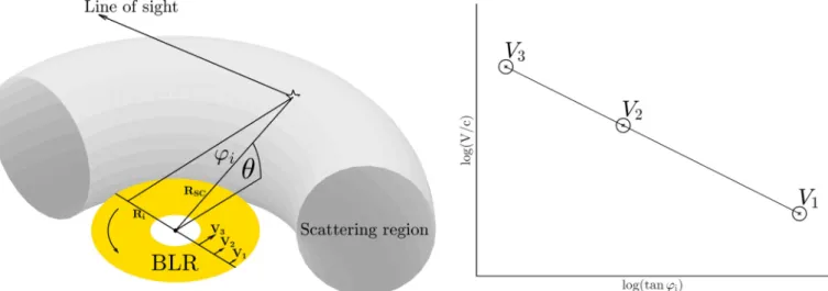
The BLR is surrounded by a co-planar scattering region (SR) that produces polarized broad lines, and a characteris-tic change in polarization plane position angle ϕ across the line profile can be expected (Smith et al. 2005). According to AP15, ϕ in the broad emission line is affected by the veloc-ity field in the BLR and has a specific linear relationship be-tween log V and log(tan ϕ). As shown in Fig. 1 (right), if we have separation in the velocity field, it will affect ϕ across the line.
Let us briefly describe the method. If the motion in the BLR is Keplerian, for the projected velocity in the plane of the scattering region, we can write (seeAfanasiev et al. 2014, AP15)
Vi= Virotcos θ=
r GMBH
Ri
cos θ, (1)
where Vi is the rotational velocity of emitting gas, MBH is the
BH mass, Ri is the distance from the center of the disk, G is
the gravitational constant, and θ is the angle between the disk and the plane of scattering (Afanasiev & Popovi´c 2015); Rican
be connected with the corresponding polarization angle ϕi as
Ri = Rsctan ϕi, where Rsc is the distance from the center to
the SR (Fig.1). When we substitute this into Eq. (1) taking into account the contribution of the different parts of the disk, the velocity-angle dependence can be transformed as
logVi
c = a − 0.5 log (tan (ϕi)), (2) where c is the speed of light. The expected relation between ve-locity and ϕ is shown in Fig.1(right). The constant a is related to the black hole mass as
a= 0.5 logGMBHcos
2θ
c2R sc
. (3)
In the case of a thin SR (equatorial scattering region), a good approximation would be to take θ ∼ 0. In this case, the rela-tion between velocities and ϕ does not depend on the inclinarela-tion since the BLR is emitting a nearly edge-on oriented line light to the SR. From the previous equation, the mass of the black hole can be calculated as MBH= 1.78 × 10²a+10 Rsc cos2θM ≈ 1.78 × 10 2a+10R sc[M ] , (4) or logMBH M = (10 + 2a) log (1.78Rsc), (5)
where Rscis in light days.
3. Simulation of equatorial scattering 3.1. Radiative transfer code
We used the radiative transfer code stokes (Goosmann & Gaskell 2007; Marin et al. 2012, 2015) to investigate polariza-tion in the broad emission line in AGNs. It is a 3D radiative transfer code based on the Monte Carlo approach. It follows single photons from their creation inside the emitting region through processes such as electron or dust scattering until they become absorbed or until they manage to reach a distant observer. Initially, it was developed to study the ultraviolet (UV) and optical continuum polarization induced by electron and dust scattering in the radio-quiet AGNs, but it is suitable for studying many astrophysical objects of various geometries (Marin & Goosmann 2014). We used the latest 1.2 version of the code stokes, which is publicly available1.
3.2. Parameters of the model
In our model, a point-like continuum source is situated in the center, emitting isotropic unpolarized radiation for which the flux is given by a power-law spectrum FC ∝ ν−α with α = 2.
Since we are investigating the spectral range around a specific line, the chosen value for the spectal index α= 2 will not affect our research.
The continuum source is surrounded by a BLR which is fi-nally surrounded by a SR. The BLR and SR are modeled using
Fig. 1.Schematic view of light being scattered from the inner part of the torus (left). Expected relation between ϕ and velocity intensity (right).
flared-disk geometry with a half-opening angle from the equato-rial plane of 15◦(covering factor ∼0.1) for the BLR and 35◦for the SR. A high covering factor for the SR is necessary in order to obtain the observed profile of the ϕ. A low covering factor of the SR gives a very small amplitude in the ϕ profile. For the BLR inner radius RBLRin , we adopted the value obtained by rever-beration mapping (Kaspi et al. 2005; Bentz et al. 2006,2013). The BLR outer radius was set by dust sublimation (predicted by
Netzer & Laor 1993) RBLRout = 0.2L
0.5
bol,46, (6)
where Lbol,46is the bolometric luminosity given in 1046ergs s−1.
Bolometric luminosity is approximated from optical nuclear luminosity (Runnoe et al. 2012)
log Liso= 4.89 + 0.91 log L5100, (7)
where log L5100is the optical nuclear luminosity. After
correct-ing for average viewcorrect-ing angle, we obtain log Lbol = 0.75 log Liso.
In our model, the BLR is transparent to photons, i.e., photons can freely travel from the inner side to the outer side of the BLR. This is in good agreement if BLR is perceived as a clumpy medium with small filling factor. For the flattened BLR (Gaskell 2009) vKepler> vturb& vinflow,
where vKepleris Keplerian velocity, vturbis the turbulence velocity,
and vinflowis the inflow velocity.
In our model, SR is a radially thin region as we assume that the light is being scattered dominantly by free electrons (Thom-son scattering) in the innermost part of the torus. We assume that the electron density is decreasing radially outwards in the form of the power law ne ∝ r−1. The SR inner radius RSRin
is found from the IR reverberation mapping (Kishimoto et al. 2011;Koshida et al. 2014). The SR outer radius RSR
out was
cho-sen such that the BLR half-opening angle when viewed from the edge of the SR is 25◦. Investigations byMarin et al.(2012)
for the SR with the flared-disk geometry have shown that opti-cally thin SR (τ ≤ 0.1) cannot produce sufficient polarization for Type-1 viewing angles. On the contrary, for optical depths τ > 3 multiple scattering can occur, resulting in depolarization. For this reason, we chose to set the total optical depth in radial direction to be τ = 1. An illustration of the model is shown in Fig.2.
Fig. 2.Model geometry of the BLR (yellow) and the scattering disk (gray) in the face-on (left) and edge-on (right) views.
3.3. Generic models
We generated four probe models for which the central SMBH has a mass of 106, 107, 108, and 109M
. We expect that the BLR
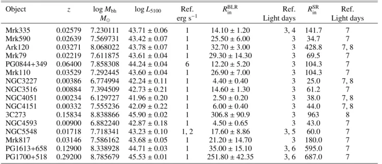
distance from the center increases when the mass of the central SMBH increases, since the mass of the SMBH scales very well with the luminosity of the AGN (Laor 2000;Gu et al. 2001). In order to determine the size and the position of the BLR, as well as the SR for our probe models, we compiled 14 AGNs for which BH masses and inner radii of the BLR and SR are known from reverberation mapping (see Table1).
We fitted the Mbh–radius relation with a power law in the
form
log MBH= C1log R+ C2, (8)
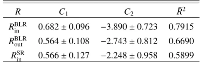
where R takes the values for RBLRin , RBLRout , and RSRin. In Fig.3, we show the mass–radius relationship with 1σ uncertainty. Fit con-stants are listed in Table2. This way we obtained a rough esti-mate of the BLR and SR sizes for our model setup. We represent the goodness of fit using the adjusted coefficient of determina-tion ¯R2.
With known fit constants, we generated values for the RBLRin , RBLRout , RSRin, and RSRout for the set of four different SMBHs (see Table 3). Our approach is the following. For each model with known input mass of the SMBH, we solve 3D radiative transfer using stokes; we then apply the AP15 method to the simulated results; and finally we compare the value of the obtained SMBH mass with the value of input SMBH mass.
Table 1. List of objects with known log Mbh, L5100, RBLRin and R SR
in that we used for models.
Object z log Mbh log L5100 Ref. RBLRin Ref. RSRin Ref.
M erg s−1 Light days Light days
Mrk335 0.02579 7.230111 43.71 ± 0.06 1 14.10 ± 1.20 3, 4 141.7 7 Mrk590 0.02639 7.569731 43.42 ± 0.07 1 25.50 ± 6.00 3 34.7 7 Ark120 0.03271 8.068022 43.78 ± 0.07 1 32.70 ± 3.00 3 428.8 7, 8 Mrk79 0.02219 7.611875 43.61 ± 0.04 1 29.30 ± 14.30 3 69.5 7 PG0844+349 0.06400 7.858308 44.24 ± 0.04 6 12.20 ± 5.20 3 104.3 7 Mrk110 0.03529 7.292445 43.60 ± 0.04 1 26.90 ± 7.00 3 104.3 7 NGC3227 0.00386 6.774994 42.24 ± 0.11 1 4.40 ± 0.40 3 25.0 7, 8 NGC3516 0.00884 7.394509 42.73 ± 0.21 1 14.60 ± 1.30 3 61.2 7 NGC4051 0.00234 6.129727 41.96 ± 0.20 1 2.50 ± 0.20 3 38.0 7, 8 NGC4151 0.00332 7.555236 42.09 ± 0.22 1 6.00 ± 0.40 3 44.0 7, 8 3C273 0.15834 8.838866 45.90 ± 0.02 1 306.8 ± 90.9 3 963 8 NGC4593 0.00900 6.882240 42.87 ± 0.18 1 4.50 ± 0.65 3 43.0 7 NGC5548 0.01718 7.718341 43.23 ± 0.10 1, 2 17.60 ± 8.86 3, 5 60.0 7 Mrk817 0.03146 7.586162 43.68 ± 0.05 1 21.20 ± 14.70 3 180.0 7 PG1613+658 0.12900 8.338928 44.71 ± 0.03 1 35.00 ± 15.10 3, 6 595.0 7 PG1700+518 0.29200 8.785679 45.53 ± 0.01 1 251.80 ± 42.35 3, 6 687.0 7
Notes. Mass was estimated from reverberation mapping using the Hβ line and for h f i= 4.3 (Grier et al. 2013).
References. Optical luminosities are taken from (1)Bentz et al.(2013), (2)Peterson et al.(2013). The estimates for RBLR
in are taken from (3)
Zu et al.(2011), (4)Grier et al.(2012), (5)Grier et al.(2013), (6)Kaspi et al.(2000). The estimates for RSR
in are taken from (7)Koshida et al.
(2014), (8)Kishimoto et al.(2011).
Fig. 3.Mass–radius relation, for RBLR in (left), R
BLR
out (middle), and RSRin (right). Data taken from literature (see Table1) are denoted as triangles; while
solid lines represent the best fit. Dashed lines mark the 1σ uncertainty.
4. Observations
We have selected four AGNs with prominent changes in ϕ across the line profile: NGC4051, NGC4151, 3C273, and PG0844+349. Spectropolarimetry was done with the 6 m tele-scope of the Special Astrophysical Observatory of the Russian Academy of Sciences (SAO RAS) using a modified version of the SCORPIO spectrograph (see Afanasiev & Moiseev 2005,
2011). Data reduction and the calculation of the polarization
parameters, as well as corrections for the interstellar polarization, aredoneinthesamewayasdescribedinAfanasiev & Amirkhanyan
(2012). Model parameters for these objects are given Table4. In order to test the AP15 method theoretically, we modeled each of these objects using observational data available from the literature. This is important since we can perform direct comparison of the results obtained from the model with the newest spectropolarimetric observations using the SAO RAS 6 m telescope. The values of RBLRin and RSRin were taken from the
Table 2. Constants C1 and C2 for the mass–radius relation (Eq. (8); Cols. 2 and 3). R C1 C2 R¯2 RBLR in 0.682 ± 0.096 −3.890 ± 0.723 0.7915 RBLRout 0.564 ± 0.108 −2.743 ± 0.812 0.6690 RSR in 0.566 ± 0.127 −2.248 ± 0.958 0.5899
Notes. Adjusted coefficient of determination ¯R2 (Col. 4) for the
per-formed fit.
Table 3. Central SMBH masses, inner and outer radius of the BLR, and inner radius of the SR that we used in our model.
Mass RBLR in R BLR out RSRin R SR out M ld ld ld ld 106 1.597 4.385 13.968 20.262 107 7.681 16.076 51.372 74.277 108 36.944 58.934 188.939 272.288 109 177.700 216.043 694.893 998.170
literature using the dust reverberation method (Kishimoto et al. 2011; Koshida et al. 2014, Table1), while RBLRout and RSRout were computed in the same way as for the generic models. Model parameters for these objects are given in Table 4. Input mass was obtained by applying the AP15 method to the observational data.
NGC 4051is a relatively nearby Seyfert 1 galaxy with cos-mological redshift equal to 0.0023, known for its highly variable X-ray flux (McHardy et al. 2004). NGC 4051 was extensively observed in the high-energy band to see if the rapid continuum variations observed in the X-ray spectra are correlated to the op-tical band fluctuations. This is not the case, even though the time-averaged X-ray and optical continuum fluxes are well correlated. Only the flux of the broad Hβ line lags behind the optical con-tinuum variations by 6 days, allowing us to estimate the mass of the central supermassive black hole (Peterson et al. 2000). The optical continuum polarization of NGC 4051 was measured by
Martin et al.(1983) andSmith et al.(2002), who found a polar-ization degree of 0.52 ± 0.09% and 0.55 ± 0.04%, respectively. The polarization position angle was found to be parallel to the radio axis of the AGN, such as expected for most Type-1 objects (Antonucci 1993).
NGC 4151 is a 1.5 Seyfert galaxy situated at z = 0.0033 (de Vaucouleurs et al. 1991), which is sometimes considered to be the archetypal Seyfert 1 galaxy (Shapovalova et al. 2008,
2010). It is one of the brightest Type-1 AGNs in the X-ray and ultraviolet band, and its bolometric luminosity is on the order of 5 × 1043 erg s−1(Woo & Urry 2002). The mass of its central
supermassive black hole was estimated by optical and ultravi-olet reverberation techniques and is estimated at 4.5 × 10⁷M
(Bentz et al. 2006). Since NGC 4151 stands out, thanks to its high fluxes and proximity, its optical polarization has been ex-tensively observed (seeMarin et al. 2016). The averaged 4000– 8000 Å continuum polarization is below 1%, with a polariza-tion posipolariza-tion angle parallel to the radio axis of the system. In the optical range, NGC 4151 shows flux variations of the con-tinuum and of the broad lines up to a factor of ten or greater (Shapovalova et al. 2008,2010). The wings of broad lines also
vary greatly from very intensive ones corresponding to type Sy1 in the maximum state of activity to almost complete absence in the minimum state of activity. In April 1984, the nucleus of NGC 4151 went through a very deep minimum, the broad wings of the hydrogen lines almost completely vanished, and the spectrum of the nucleus was identified as a Sy 2 (Penston & Perez 1984). In this phase, the intensity in the broad component of a spectral line is too weak and the AP15 method probably could not be used. Another technique must be used to explore the geometry of the object, such as proved byHutsemékers et al.(2017) and
Marin(2017).
3C 273 is a well-known flat-spectrum radio source quasar with broad emission lines. It is the brightest and one of near-est quasars known to us (z = 0.158, Courvoisier et al. 1987,
1990). It is a radio-loud object, i.e., its radio to millimeter en-ergy output is dominated by synchrotron emission from a kilo-parsec, one-sided jet whose emission extends up to the infrared and optical bands. 3C 273 is particularly bright in the optical and ultraviolet domains, which enabled the detection of the po-larization of the optical emission. Its mean optical core polar-ization was measured byAppenzeller(1968) and is on the order of 0.2 ± 0.2%, which is consistent with galactic interstellar po-larization (Whiteoak 1966). The optical polarization emerging from the jet structure is high because they were resolved into a number of highly polarized knot structures byThomson et al.
(1993). Nevertheless, Balmer emission lines were first measured bySchmidt(1963) and allowed the central black hole mass to be determined from the average line profiles (Kaspi et al. 2000).
PG0844+349 is a radio-quiet quasar at a cosmological red-shift of z = 0.064 that, unlike most quasars, was not origi-nally detected in the radio frequency: at radio wavelengths, its nucleus is unresolved (Kellermann et al. 1994). It was first dis-covered in the Palomar Green sample (Schmidt & Green 1983) and was found to possess strong Fe II emission and weak for-bidden narrow lines, a behavior that is expected from narrow-line Seyfert-1s (NLS1). On the other hand, the X-ray proper-ties of PG 0844+349 are aligned with the NLS1 classification (a steep soft X-ray spectrum and strong variability, seeBoller 2001), and the optical polarization measurements achieved by
Afanasiev et al.(2011) also point towards a regular NLS1 object (optical continuum polarization of 0.85 ± 0.10%). Hence, using Type-1 AGN reverberation mapping techniques,Peterson et al.
(2004) estimated the mass of the central black hole to be (9.24 ± 3.81) × 108M
.
5. Results
We present our results which can be divided into two parts: the results of modeling and a comparison of our models with the ob-servations. The same convention used byGoosmann & Gaskell
(2007) was adopted in this work. Namely, ϕ is parallel to the symmetry axis of the model when ϕ= 90◦, which was observed
for Type-1 objects, or ϕ is orthogonal to the symmetry axis when ϕ = 0◦, which was observed for Type-2 objects.
5.1. Generic modeling
We simulated different geometries of the BLR. We first per-formed the simulation for different masses of the black holes with assumption of a pure Keplerian motion, and then we con-sidered the radial inflow and vertical outflow as additional com-ponents in gas motion to the Keplerian caused by the black hole mass. We simulated both cases where Keplerian motion is coun-terclockwise (positive) and clockwise (negative).
Table 4. Central SMBH masses, inner and outer radius of the BLR and SR that we used in our model for comparison with the observed data.
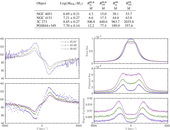
Object Log(MPOL/M ) RBLRin RBLRout RSRin R SR out ld ld ld ld NGC 4051 6.69 ± 0.21 4.3 15.0 38.1 53.7 NGC 4151 7.21 ± 0.27 6.6 17.5 44.0 63.8 3C 273 8.85 ± 0.27 306.8 440.6 963.7 2035.8 PG0844+349 7.70 ± 0.14 12.2 77.4 189.0 357.6
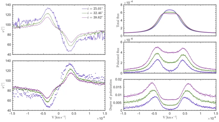
Fig. 4.Left panels: modeled polarization plane position angle ϕ when the system is rotating counterclockwise (top) or when rotating clockwise (bottom). Right panels: total unpolarized flux (TF, top), polarized flux (PF, middle), degree of polarization (PO, bottom). The SMBH has a mass of 106 M
. We plot the results in solid lines for three viewing inclinations: i= 25.01◦, 32.46◦, and 38.62◦, while dotted lines represent the results
for the opposite direction of rotation. We note the symmetry of ϕ with respect to the continuum level, due to the opposite direction of rotation. An opposite direction of rotation does not affect TF, PF, and PO. Total and polarized fluxes are given in arbitrary units.
5.1.1. Pure Keplerian gas motion in the BLR
We consider the pure Keplerian motion of the BLR emitting gas, taking that there are no other effects (e.g., outflows and inflows). We present the results of the four probe models. In Figs. 4 and5, we show the simulated profiles of ϕ, polarized flux (PF), degree of polarization (PO), and total flux (TF) across the broad-line profile. Each scattering element can see the ve-locity resolved BLR emission which produces polarized lines that are broader than the unpolarized lines. The simulated de-gree of polarization is of the same order of magnitude as that obtained from the observations and is typically around 1% or less (Marin et al. 2016). From our models (Figs. 4and5, bot-tom right panels), we can see that the degree of polarization is sensitive to inclination. Extensive modeling with complex radi-ation reprocessing (see, e.g.,Marin et al. 2012, for more details) have shown that the total PO is increasing as we start looking from the face-on viewing angle towards Type-2 viewing angles. Although we included only equatorial scattering in our model, the dependence of PO on inclination follows this trend. The PO profile peaks in the line wings and reaches a minimum in the
line core, as was shown bySmith et al.(2005). This feature was very well observed for the case of Mrk 6 (Smith et al. 2002;
Afanasiev et al. 2014) and it supports the suggested scattering geometry.
The polarization plane position angle is aligned with the disk rotation axis, hence also with the radio jet axis. In Figs.4and5
(left panels), we show the simulated profiles of ϕ for three view-ing inclinations. The ϕ profiles show a typical symmetric swview-ing that was predicted for Type-1 objects where the radiation from the Keplerian rotating disk-like BLR is being scattered by the outer dusty torus (Smith et al. 2005, AP15). The direction of ro-tation only affects ϕ, while TF, PF, and PO remain unaffected. For counterclockwise rotation, ϕ reaches a maximum value in the blue part of the line and minimum in the red part of the line. The ϕ swing occurs around the level of continuum ϕc = 90◦.
Due to the symmetry of the model (also for all other models performed in the paper), ϕ is symmetric with respect to the con-tinuum polarization in such a way that for a given inclination i, it satisfies the following:
ϕ(180◦
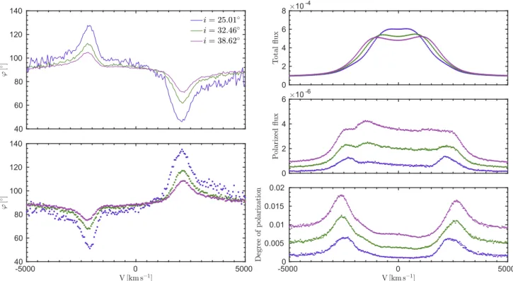
Fig. 5.Same as Fig.4, but for SMBH of 109M .
In other words, for a given half-opening angle of the torus θ0, and
for Type-1 inclinations where 0 ≤ i ≤ 90◦−θ0, the observer can
see one way of rotation, and the corresponding ϕ profile will be as shown in Figs.4and5. If the system is viewed for the Type-1 viewing angle where 90◦+ θ
0≤ i ≤ 180◦, the opposite direction
of rotation is observed and the resulting ϕ satisfies Eq. (9). This symmetry can be seen in Figs.4and5(left panels). Thus, spec-tropolarimetric observations of Type-1 Seyferts can disentangle the rotation direction of the gas by observing the ϕ profile. Equa-tion9is satisfied within the Monte Carlo uncertainty and it was used to improve photon statistics in our simulations by a factor of 2 by simply taking the average value of the Stokes parameters for inclinations i and 180◦− i.
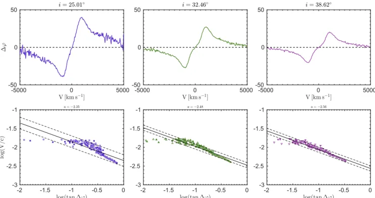
When applying the AP15 method to the modeled data, we needed to consider polarization only in the broad line; thus, it was necessary to subtract the continuum polarization for all Type-1 inclinations:
∆ϕ = ϕ − 90◦. (10)
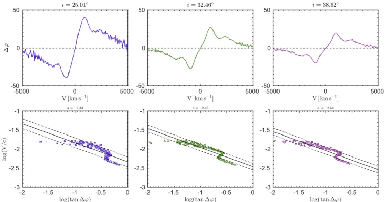
Since all of our observed objects are rotating clockwise (see Sect.5.2), we performed the AP15 method assuming the oppo-site direction of rotation without introducing new simulations. In Fig.6(lower panels), we show the fit described by the AP15 method. We find that Keplerian motion can be traced across the ϕ profile for Type-1 viewing inclinations. The region inside the 1σ error around the linear fit becomes smaller as we go from face-on towards edge-face-on inclinatiface-ons. For inclinatiface-ons 25◦ or lower,
the simulated data show much higher scatter around the straight line rather than for the cases with an average inclination.
The effect of a wide SR (in our case θ0 = 35◦) can lead to
mass estimates that are a maximum of ∼1.5 higher than those obtained for equatorial scattering, and only if the SR lies much farther away from the BLR (see Eq. (4)). In this case, the influ-ence of the viewing inclination must be taken into account.
It is important to note that in Eq. (4), we used the inner radius of the SR in order to estimate the mass of the SMBH. However,
Table 5. Input mass (Col. 1), viewing inclinations (Col. 2), and masses obtained for probe models (Col. 3).
log Minput i(◦) log(MMOD/M )
25.01 6.72 ± 0.10 6 32.46 6.44 ± 0.06 38.62 6.28 ± 0.05 25.01 7.59 ± 0.10 7 32.46 7.30 ± 0.07 38.62 7.17 ± 0.04 25.01 8.65 ± 0.11 8 32.46 8.39 ± 0.07 38.62 8.23 ± 0.06 25.01 9.67 ± 0.16 9 32.46 9.43 ± 0.12 38.62 9.27 ± 0.10
Notes. Masses are given in M .
the SR does not act as a mirror from which the light is being scattered from the inner wall. Scattering events occur in the en-tire SR, and they all contribute to the total ϕ shape. Obtaining the value for parameter a is a straightforward procedure, but the final estimated SMBH value largely depends on the actual value of Rsc. In the optically thick media, the largest fraction of
pho-tons is scattered from the inner side of the SR.
One of the factors that has significant impact on the ϕ amplitude is the mutual distance between the BLR and the SR (Smith et al. 2005). The amplitude of ϕ decreases when mutual distance increases, which affects black hole mass esti-mation. Therefore, we investigated different cases with various mutual distances between the BLR and SR, while keeping the same thickness and optical depth as the SR. In Figs.7and8, we show the influence of different mutual distance between the two regions, and how it affects the parameter a and SMBH estimates.
Fig. 6.Modeled polarization ϕ (upper panels) and velocities (lower panels) across Hα profiles for the model with central mass of 106 M . Filled
symbols are for the blue part of the line and open symbols are for the red part of the line. The solid line represents the best fit.
Our models show that the mutual distance between the BLR and SR has a great influence on the parameter a, which consequently greatly affects our black hole mass estimates. Parameter a shows the same profile and the same inclination dependence for all sim-ulated cases. Only when the SR is adjacent to the BLR do we ob-tain inclination independence of the SMBH mass estimates. Due to the nature of Eq. (4), SMBH mass estimates increase when the mutual distance increases. For a given accuracy of 10%, we find that the best SMBH estimates for all four cases are when the ratio of the inner radius of SR and the outer radius of the BLR is between 1.5 and 2.5 (Fig.8). For the inclinations of 25◦ or less
(face-on view), the contribution of equatorial scattering is low and we find that Keplerian motion cannot be recovered from the ϕ profile.
5.1.2. Keplerian motion and radial inflow
We investigated a particular case when the BLR is undergo-ing a constant radial inflow. We tested three cases with BLR radial inflow velocity equal to 500 km s−1, 1000 km s−1, and
2000 km s−1. As before, in Fig. 9we show simulated profiles of ϕ, PF, PO, and TF. In this regime, the SR can see an addi-tional component of the BLR velocity, which as a net effect increases the absolute value of the radial velocity that a single scattering element can see. This leads to additional line broad-ening (Fig.9, lower right panel) when compared to the case with pure gas Keplerian motion only. As a resulting effect, the distance between the positions of the maximum and the minimum of the ϕ is increased (Fig.9, left panels). Therefore, for a low-velocity radial inflow, mass estimates of the SMBHs are slightly higher than those obtained in the case with Keplerian motion alone. This overestimation of the SMBH mass mostly affects the model for which the SMBH has a mass of 106 M
. For the other models,
Keplerian motion is even more dominant (except for the very extreme cases which are not expected) and the influence of the radial inflow can be neglected.
5.1.3. Keplerian motion and vertical outflow
Another contribution to velocity might be due to vertical outflows. We tested three cases for which the innermost one-third of the BLR is undergoing a constant vertical outflow of 500 km s−1, 1000 km s−1, and 2000 km s−1. In this case, the equatorial
scat-tering elements will not see this velocity component. Scatscat-tering elements above the equatorial plane will see this component mul-tiplied by a factor of cos α, where α is latitude, to a maximum of cos 35◦. This can be neglected when the outflow velocity is much lower than Keplerian velocity. In Fig.10, we show the re-sults of simulated ϕ, PF, PO, and TF influenced by vertical out-flows in the BLR of 2000 km s−1for the case where SMBH has a
mass of 106M . The unpolarized line (bottom right panel) is
ad-ditionally broadened in the wings. The polarized line (upper right panel) is almost the same as the one for the case with Keplerian motion only (Fig.4, upper right panel), for the reasons explained above. Contribution of outflow velocity is highest for the nearly face-on view. In Fig.11, left panels, the ϕ profile shows an ad-ditional bump, which prevents us from correctly using the AP15 method. We would like to point out again that in our model, the BLR is transparent and that the observer can see the radiation com-ing from the approachcom-ing and the recedcom-ing part of the BLR out-flows. We know from observations that this is not the case (e.g., Mrk 6;Afanasiev et al. 2014), and we expect to observe radia-tion from the approaching side of the BLR outflows, while the radiation from the receding side of the BLR outflows should be blocked, thus affecting only the blue part of the line.
5.2. Comparison with observations
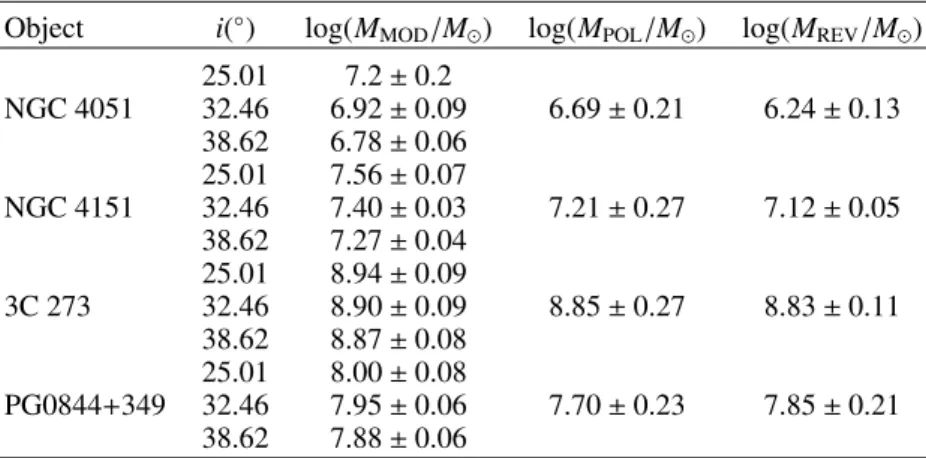
Here we present the fits of our model with observations in order to estimate the SMBH mass. We fit model data to observational data and compare the results, The results are given in Table6, and below we discuss the results and visual comparison for each object.
Fig. 7.Dependence of the parameter a on the ratio between the inner radius of the SR (RSR
in) and the outer radius of the BLR (R BLR
out ) for three given
inclinations.
Fig. 8.Black hole mass estimation as a function of the ratio between the inner radius of the SR (RSR
in) and the outer radius of the BLR (R BLR out ) for
Fig. 9.Same as Fig.4, but in addition to Keplerian motion, a large inflow of 2000 km s−1is included in the BLR kinematics.
Fig. 10.Same as Fig.4, except that here the inner one-third of the BLR undergoes a constant vertical outflow of 2000 km s−1.
NGC 4051 – We were able to obtain the expected ϕ shape (Fig.12, upper panels).
The amplitude of the ϕ in the model is very close to the observed value for the lowest inclination for which i = 25.01◦. For this
inclination, the position of the maximum and the minimum of ϕ is displaced, which yields the highest mass estimate. As we start viewing from higher inclinations, the ϕ amplitude decreases and we are able to better fit the line wings (Fig.12, lower panels), and the difference between the estimated values of the SMBH masses
and the input mass is smaller. We can see that simulated data in the line wings for i= 25◦deviate from the theoretically predicted straight line. For intermediate inclinations the 1σ offset is smaller and the fit is better.
Similarly, SMBH masses estimated from the fitting of the model data are higher than the input mass, as in the previous case. For this object, RSRin/RBLRout ≈ 2.54.
NGC 4151– Similarly to the previous case, we obtain the high-est mass high-estimate for the lowhigh-est inclination. Keplerian motion is
Fig. 11.Same as Fig.6, except that here the inner one-third of the BLR undergoes a constant vertical outflow of 2000 km s−1.
Fig. 12.Modeled broad-line polarization position angle ϕ (upper panels) and velocities (lower panels) across Hα profiles for NGC 4051. In the upper panels, data obtained by the models are depicted as a line, while observed data are depicted by empty circles. In the lower panels, filled symbols are for the blue part of the line and the open symbols are for the red part of the line for model data. Black circles depict observed data. The solid black line represents the best fit. Values of the parameter a, correlation coefficient r, and the corresponding p values are shown.
shown very well as a straight line (Fig.A.1, lower panels), where the 1σ error is small, especially in the case where i = 39◦. For
this object, RSRin/RBLRout ≈ 2.51.
We can see that in the extreme wings of the line, the modeled ϕ becomes very sensitive to spectral resolution and this sensitivity is lower for higher inclinations.
3C 273 – We obtained very low ϕ dependence on inclina-tion; however, the ϕ amplitude is much smaller, around 19◦
for all inclinations (Fig. A.2). Model data show a deviation from the straight line in the line wings; however, the scatter is much smaller than it is for the observational data. The ratio RSR
in /R BLR
Table 6. Viewing inclinations, SMBH masses estimates from model (Col. 3), from observations (Col. 4), and from reverberation mapping (Col. 5).
Object i(◦) log(M
MOD/M ) log(MPOL/M ) log(MREV/M )
25.01 7.2 ± 0.2 NGC 4051 32.46 6.92 ± 0.09 6.69 ± 0.21 6.24 ± 0.13 38.62 6.78 ± 0.06 25.01 7.56 ± 0.07 NGC 4151 32.46 7.40 ± 0.03 7.21 ± 0.27 7.12 ± 0.05 38.62 7.27 ± 0.04 25.01 8.94 ± 0.09 3C 273 32.46 8.90 ± 0.09 8.85 ± 0.27 8.83 ± 0.11 38.62 8.87 ± 0.08 25.01 8.00 ± 0.08 PG0844+349 32.46 7.95 ± 0.06 7.70 ± 0.23 7.85 ± 0.21 38.62 7.88 ± 0.06
Notes. MPOLdenotes masses obtained using AP15 which we used as input mass. Masses obtained by reverberation mapping were taken from
Bentz & Katz(2015) using virial factor h f i= 4.31 ± 1.05 (Grier et al. 2013).
Mass estimates follow the previous trend: the highest estimate for the lowest inclination.
PG0844+349 – We can see from observations that the ϕ profile is asymmetric and that the ϕ amplitude is greater for the red part of the line than for the blue part. The results are similar to those of the first two objects (Fig.A.3), RSRin /RBLRout ≈ 2.44.
For all modeled objects, we were able to produce profiles of ϕ that were very similar to the observed profiles (Figs.12,A.1,
A.2,A.3, upper panels). The SMBH masses estimated from the fitting of the model data are higher than those obtained by fit-ting the observational data, and the obtained values decrease as the viewing inclination increases (Table 6); the ϕ amplitude is very sensitive to inclination and decreases when viewing from face-on towards edge-on inclinations (from lower to greater). For all observed objects, the modeled PO ranges from 0.5% to 1.5% for inclinations from lowest to highest. As a measure of the strength of a linear association between the model data and the fit, we give the values of the Pearson correlation coefficient r. For all objects we find that the correlation coefficient r is greater than 0.9, except for NGC4151 when viewed from inclination i = 25.01◦ (Fig.A.1, lower left panel). The corresponding p values are very close to 0, indicating a strong linear connection between the modeled data and the fit.
The observational data are much more scattered from the predicted straight line. In general, this yields an error in SMBH estimates that is few times greater than the error obtained by re-verberation mappingAfanasiev & Popovi´c(2015). In the case of NGC 4051 and NGC 4151, modeled data show the best fits for the highest inclination (Figs.12,A.1, bottom right panels), or is in offset when viewing more towards face-on (Figs.12,A.1, bot-tom left and middle panels). The 1σ uncertainty is smaller for intermediate inclinations. The largest overestimate of the mass (a factor of 3) is for NGC4051 for i = 25◦. For all models RSR
in /R BLR
out > 2. This falls in the regime where the SMBH mass
estimation shows dependence on inclination. We achieve the best SMBH mass estimates for inclinations i ≈ 39◦, which is close to the value of an average inclination (i = 39◦) for Type-1 objects
(Lewis et al. 2010;Hryniewicz & Czerny 2012). 6. Discussion
Previous spectropolarimetric studies of Type-1 Seyferts have shown that the polarization signature across the broad Hα varies
widely from object to object (Smith et al. 2002). At intermedi-ate viewing inclinations, equatorial scattering dominintermedi-ates the ob-served polarization and the wavelength averaged polarization ϕ is closely aligned with the projected radio source axis. In their original model,Smith et al.(2005), used a single-scattering ap-proximation, i.e., photons emitted from the BLR are scattered only once from the SR before finally reaching the observer. In their model, the SR is optically thin and we find that an opti-cal depth of at least 1 along with the higher covering factor of the SR is required in order to obtain ϕ and PO comparable with observations.
In our Monte Carlo simulations, the treatment of multi-ple scattering events was fully performed and we find that the largest fraction of photons is scattered only once, while the other, smaller fraction of photons undergoes a backward scattering from one side of the SR to the other. This secures good circumstances for the application of the AP15 method. In our model, we approximated the emission of an accretion disk as a point source of isotropic continuum emission. We know that this is not the case and that anisotropy arises due to change in the projected surface area and to limb darkening effects (Netzer 1987). The strongest emission is in the direc-tion perpendicular to the disk and rapidly decreases towards edge-on viewing angles. The inner radius of the SR thus can-not be constant, and should follow a dependence on the polar angle that is similar to that of the disk emission (Stalevski et al. 2016). Silicate and graphite dust grains have different sublima-tion temperatures. Graphite grains can survive up to ∼1900 K and therefore reach closer than silicates which are destroyed when the temperature is ∼1200 K. Furthermore, smaller dust grains are destroyed at lower temperatures than the larger grains (Draine 1984;Draine & Lee 1984;Barvainis 1987). Therefore, we can expect an entire sublimation zone, from graphite to sil-icate and from larger to smaller dust grains (Kishimoto et al. 2007;Mor & Netzer 2012). This gives the opportunity for dust particles to inhabit the equatorial region in the close vicin-ity of the BLR. Equatorial scattering of broad lines from the adjacent SR gives a very low inclination dependence on the parameter a rendering the AP15 method inclination indepen-dent.
For SMBH mass estimates using the AP15 method, the inner radius of the torus is needed. It can be obtained directly using dust reverberation in the infrared (Kishimoto et al. 2011).
The number of objects for which dust reverberation has been performed is smaller than the number of objects for which the reverberation have been performed in the optical. For most of the objects, RSR
in can be calculated only through scaling
rela-tions, which can additionally increase an error in the SMBH estimates. The other way is to calculate RSRin from the UV ra-diation (Barvainis 1987). For this we need to know a priori the physical and chemical composition of dust. Using the right value is important since the estimated BH mass is directly proportional to the inner radius.
Seyfert 1 galaxies are often highly variable and when they are in a state of minimum activity (up to Type-2), the shape of the position angle of the polarization plane cannot be detected because of the weakness or absence of a flux from the broad line. In this case, the mass estimation using the AP15 method is not applicable, even if the object is confidently assigned to the type of objects with equatorial scattering. Therefore, in fu-ture modeling, the variability of an AGN must be taken into account.
Originally the AP15 method was proposed for systems with an inclination between 20◦ and 70◦. For high viewing
inclinations, we have Type-2 objects for which polar scat-tering dominates the polarization signal and the method is no longer valid. For almost pole-on AGN, the AP15 method faces two problems. First, the amount of interstellar polar-ization can dominate over the amount of scattering-induced radiation from the innermost regions of AGN. The amount of interstellar polarization is wavelength-dependent and is of-ten maximum in the optical band (see Serkowski et al. 1975). Since the polarization signal of polar AGN in the optical band is usually much lower than 1% in the optical (Smith et al. 2002; Marin 2014), the AP15 method is thus restricted to inclinations higher than 20◦. Second, the method over-estimates the SMBH mass by a factor of 1.5 in compari-son with the value obtained for the lowest inclination when RSR
in /R BLR
out ≈ 2. When the SR is closer, the inclination effect is
lower and the mass estimates only depend on the SR inner ra-dius.
It is important to note here that several recent works (Piotrovich et al. 2015; Baldi et al. 2016; Songsheng & Wang 2018) give some ideas for using spectropolarimetry to estimate BH mass in AGNs. Basically, all these papers try to constrain the virial factor (Piotrovich et al. 2015; Songsheng & Wang 2018) or to use the broad polarized line (Baldi et al. 2016) to find the black hole mass. In the work bySongsheng & Wang(2018), the authors performed Monte Carlo simulations for a wide range of parameters assuming a static flared-disk geometry for the equa-torial region. In comparison to the unpolarized spectra, the virial factor of the polarized spectra has a much narrower distribu-tion. Furthermore, the half-opening angle of the BLR and the nucleus inclinations appear to be the two parameters with the highest influence on the virial factor. The difference between the methods mentioned above and AP15 is that the AP15 method provides a direct measurement of the BH mass from the polar-ization angle, and here we also used some approaches similar to those used in Songsheng & Wang(2018), but focusing on a polarization plane position angle ϕ and the limits of the AP15 method. In comparison, our 3D polarized radiative transfer sim-ulations have shown that the polarization plane position angle is largely affected by the distance between the BLR and SR. If the two share similar values, the mass estimated using the AP15 method becomes inclination independent, which is a great advantage in comparison to traditional reverberation mapping techniques.
7. Conclusions
We modeled polarization effects in AGN broad lines in order to constrain the limits of the AP15 method for the BH estimates using polarization in broad lines.
We used the Monte Carlo radiative transfer code stokes, which includes multiple scattering for accurate polarization treatment. We considered equatorial scattering (on the torus) of the light from a BLR that has dominant Keplerian motion. Addi-tionally, we considered complex BLR kinematics having inflows and outflows.
We explored all these effects on the accuracy of the BH mass measurement using the AP15 method.
From our investigation we can outline following conclusions: – If Keplerian motion can be traced through the polarized line profile, then direct estimates of the mass can be performed to obtain reasonable values.
– The effects of possible inflow/outflow configuration of the BLR take its toll only for extreme cases where the velocity of the inflowing/outflowing emitter is comparable to or higher than the Keplerian velocity.
– Masses of the SMBHs obtained by the AP15 method are in good agreement with those found in the literature.
The AP15 method gives us a new independent way of mass estimation. Future parameter grids will be extended with the inflow/outflow configuration of the scattering region with the possibility of considering clumpy structures. We expect to per-form quality spectropolarimetric observations of the high-redshifted quasars and to test the AP15 method on highly ionized lines such as C III and C IV.
Acknowledgements. We thank an anonymous referee for the constructive sug-gestions that improved this paper. This work was supported by the Ministry of Education and Science (Republic of Serbia) through the project Astrophysical Spectroscopy of Extragalactic Objects (176001), the French PNHE and the grant ANR-11-JS56-013-01 “POLIOPTIX”, and the Russian Foundation for Basic Re-search grant N15-02-02101 and N14-22-03006. D. Savi´c thanks the French Gov-ernment and the French Embassy in Serbia for supporting his research. Part of this work was supported by the COST Action MP1104 “Polarization as a tool to study the solar system and beyond”.
References
Afanasiev, V. L., & Amirkhanyan, V. R. 2012,Astrophys. Bull., 67, 438
Afanasiev, V. L., & Moiseev, A. V. 2005,Astron. Lett., 31, 194
Afanasiev, V. L., & Moiseev, A. V. 2011,Baltic Astron., 20, 363
Afanasiev, V. L., & Popovi´c, L. ˇC. 2015,ApJ, 800, L35
Afanasiev, V. L., Borisov, N. V., Gnedin, Y. N., et al. 2011,Astron. Lett., 37, 302
Afanasiev, V. L., Popovi´c, L. ˇC., Shapovalova, A. I., Borisov, N. V., & Ili´c, D. 2014,MNRAS, 440, 519
Antonucci, R. 1993,ARA&A, 31, 473
Appenzeller, I. 1968,ApJ, 151, 769
Baldi, R. D., Capetti, A., Robinson, A., Laor, A., & Behar, E. 2016,MNRAS, 458, L69
Barvainis, R. 1987,ApJ, 320, 537
Bentz, M. C., & Katz, S. 2015,PASP, 127, 67
Bentz, M. C., Denney, K. D., Cackett, E. M., et al. 2006,ApJ, 651, 775
Bentz, M. C., Denney, K. D., Grier, C. J., et al. 2013,ApJ, 767, 149
Blandford, R. D., & McKee, C. F. 1982,ApJ, 255, 419
Boller, T. 2001, in New Century of X-ray Astronomy, eds. H. Inoue & H. Kunieda,ASP Conf. Ser., 251, 112
Courvoisier, T. J.-L., Turner, M. J. L., Robson, E. I., et al. 1987,A&A, 176, 197
Courvoisier, T. J. L., Robson, E. I., Blecha, A., et al. 1990,A&A, 234, 73
de Vaucouleurs, G., de Vaucouleurs, A., Corwin, Jr. H. G., et al. 1991,S&T, 82, 621
Draine, B. T. 1984,ApJ, 277, L71
Draine, B. T., & Lee, H. M. 1984,ApJ, 285, 89
Fabian, A. C. 2012,ARA&A, 50, 455
Ferrarese, L., & Ford, H. 2005,Space Sci. Rev., 116, 523
Gaskell, C. M. 2009,New Astron. Rev., 53, 140
Gebhardt, K., Bender, R., Bower, G., et al. 2000,ApJ, 539, L13
Genzel, R., Eisenhauer, F., & Gillessen, S. 2010,Rev. Mod. Phys., 82, 3121
Goosmann, R. W., & Gaskell, C. M. 2007,A&A, 465, 129
Grier, C. J., Peterson, B. M., Pogge, R. W., et al. 2012,ApJ, 755, 60
Grier, C. J., Martini, P., Watson, L. C., et al. 2013,ApJ, 773, 90
Gu, M., Cao, X., & Jiang, D. R. 2001,MNRAS, 327, 1111
Heckman, T. M., & Best, P. N. 2014,ARA&A, 52, 589
Hryniewicz, K., & Czerny, B. 2012,Mem. Soc. Astron. It., 83, 146
Hutsemékers, D., Agís González, B., Sluse, D., Ramos Almeida, C., & Acosta Pulido J.-A. 2017,A&A, 604, L3
Kaspi, S., Smith, P. S., Netzer, H., et al. 2000,ApJ, 533, 631
Kaspi, S., Maoz, D., Netzer, H., et al. 2005,ApJ, 629, 61
Kellermann, K. I., Sramek, R. A., Schmidt, M., Green, R. F., & Shaffer, D. B. 1994,AJ, 108, 1163
Kishimoto, M., Hönig, S. F., Beckert, T., & Weigelt, G. 2007,A&A, 476, 713
Kishimoto, M., Hönig, S. F., Antonucci, R., et al. 2011,A&A, 536, A78
Kormendy, J., & Ho, L. C. 2013,ARA&A, 51, 511
Kormendy, J., & Richstone, D. 1995,ARA&A, 33, 581
Koshida, S., Minezaki, T., Yoshii, Y., et al. 2014,ApJ, 788, 159
Krolik, J. H., & Begelman, M. C. 1988,ApJ, 329, 702
Laor, A. 2000,ApJ, 543, L111
Lewis, K. T., Eracleous, M., & Storchi-Bergmann, T. 2010,ApJS, 187, 416
Lynden-Bell, D. 1969,Nature, 223, 690
Marin, F. 2014,MNRAS, 441, 551
Marin, F. 2017,A&A, 607, A40
Marin, F., & Goosmann, R. W. 2014, inSF2A-2014: Proceedings of the Annual Meeting of the French Society of Astronomy and Astrophysics, eds. J. Ballet, F. Martins, F. Bournaud, R. Monier, & C. Reylé, 103
Marin, F., Goosmann, R. W., Gaskell, C. M., Porquet, D., & Dovˇciak M. 2012,
A&A, 548, A121
Marin, F., Goosmann, R. W., & Gaskell, C. M. 2015,A&A, 577, A66
Marin, F., Goosmann, R. W., & Petrucci, P.-O. 2016,A&A, 591, A23
Martin, P. G., Thompson, I. B., Maza, J., & Angel, J. R. P. 1983,ApJ, 266, 470
McHardy, I. M., Papadakis, I. E., Uttley, P., Page, M. J., & Mason, K. O. 2004,
MNRAS, 348, 783
Meyer, L., Ghez, A. M., Schödel, R., et al. 2012,Science, 338, 84
Miyoshi, M., Moran, J., Herrnstein, J., et al. 1995,Nature, 373, 127
Mor, R., & Netzer, H. 2012,MNRAS, 420, 526
Netzer, H. 1987,MNRAS, 225, 55
Netzer, H. 2013, The Physics and Evolution of Active Galactic Nuclei
(Cambridge, UK: Cambridge University Press) Netzer, H., & Laor, A. 1993,ApJ, 404, L51
Penston, M. V., & Perez, E. 1984,MNRAS, 211, 33
Peterson, B. M. 2014,Space Sci. Rev., 183, 253
Peterson, B. M., McHardy, I. M., Wilkes, B. J., et al. 2000,ApJ, 542, 161
Peterson, B. M., Ferrarese, L., Gilbert, K. M., et al. 2004,ApJ, 613, 682
Peterson, B. M., Denney, K. D., De Rosa, G., et al. 2013,ApJ, 779, 109
Piotrovich, M. Y., Gnedin, Y. N., Silant’ev, N. A., Natsvlishvili, T. M., & Buliga, S. D. 2015,MNRAS, 454, 1157
Runnoe, J. C., Brotherton, M. S., & Shang, Z. 2012,MNRAS, 427, 1800
Schmidt, M. 1963,Nature, 197, 1040
Schmidt, M., & Green, R. F. 1983,ApJ, 269, 352
Serkowski, K., Mathewson, D. S., & Ford, V. L. 1975,ApJ, 196, 261
Shapovalova, A. I., Popovi´c, L. ˇC., Collin, S., et al. 2008,A&A, 486, 99
Shapovalova, A. I., Popovi´c, L. ˇC., Burenkov, A. N., et al. 2010,A&A, 509, A106
Smith, J. E., Young, S., Robinson, A., et al. 2002,MNRAS, 335, 773
Smith, J. E., Robinson, A., Young, S., Axon, D. J., & Corbett, E. A. 2005,
MNRAS, 359, 846
Songsheng, Y.-Y., & Wang, J.-M. 2018,MNRAS, 473, L1
Stalevski, M., Ricci, C., Ueda, Y., et al. 2016,MNRAS, 458, 2288
Thomson, R. C., Mackay, C. D., & Wright, A. E. 1993,Nature, 365, 133
Urry, C. M., & Padovani, P. 1995,PASP, 107, 803
Whiteoak, J. B. 1966,Z. Astrophys., 64, 181
Woo, J.-H., & Urry, C. M. 2002,ApJ, 579, 530
Appendix A: Additional figures
Fig. A.1.Same as in Fig.12, but for NGC4151.