HAL Id: hal-00296237
https://hal.archives-ouvertes.fr/hal-00296237
Submitted on 24 May 2007
HAL is a multi-disciplinary open access
archive for the deposit and dissemination of
sci-entific research documents, whether they are
pub-lished or not. The documents may come from
teaching and research institutions in France or
abroad, or from public or private research centers.
L’archive ouverte pluridisciplinaire HAL, est
destinée au dépôt et à la diffusion de documents
scientifiques de niveau recherche, publiés ou non,
émanant des établissements d’enseignement et de
recherche français ou étrangers, des laboratoires
publics ou privés.
Ny-Ålesund, Svalbard based on 15 years of radiosonde
data
R. Treffeisen, R. Krejci, J. Ström, A. C. Engvall, A. Herber, L. Thomason
To cite this version:
R. Treffeisen, R. Krejci, J. Ström, A. C. Engvall, A. Herber, et al.. Humidity observations in the
Arctic troposphere over Ny-Ålesund, Svalbard based on 15 years of radiosonde data. Atmospheric
Chemistry and Physics, European Geosciences Union, 2007, 7 (10), pp.2721-2732. �hal-00296237�
www.atmos-chem-phys.net/7/2721/2007/ © Author(s) 2007. This work is licensed under a Creative Commons License.
Chemistry
and Physics
Humidity observations in the Arctic troposphere over Ny- ˚
Alesund,
Svalbard based on 15 years of radiosonde data
R. Treffeisen1, R. Krejci2, J. Str¨om3, A. C. Engvall2, A. Herber4, and L. Thomason5
1Alfred Wegener Institute for Polar and Marine Research, Telegrafenberg A45, 14473 Potsdam, Germany 2Department of Meteorology (MISU), Stockholm University, S 106 91 Stockholm, Sweden
3ITM – Department of Applied Environmental Science, Stockholm University, S 106 91 Stockholm, Sweden 4Alfred Wegner Institute for Polar and Marine Research, Am Handelshafen 12, 27570 Bremerhaven, Germany 5NASA Langley Research Center Hampton, VA 23681-2199, USA
Received: 30 November 2006 – Published in Atmos. Chem. Phys. Discuss.: 25 January 2007 Revised: 26 March 2007 – Accepted: 14 May 2007 – Published: 24 May 2007
Abstract. Water vapour is an important component in the
radiative balance of the polar atmosphere. We present a study covering fifteen years of data of tropospheric humidity profiles measured with standard radiosondes at Ny- ˚Alesund (78◦55′N 11◦52′E) during the period from 1991 to 2006. It is well-known that relative humidity measurements are less reliable at low temperatures when measured with standard radiosondes. The data was corrected for errors and used to determine key characteristic features of the vertical and tem-poral relative humidity evolution in the Arctic troposphere over Ny- ˚Alesund. We present frequencies of occurrence of ice-supersaturation layers in the troposphere, their vertical span, temperature and statistical distribution. Supersatura-tion with respect to ice shows a clear seasonal behaviour. In winter, (October–February) it occurred in 19% of all cases and less frequently in spring (March–May 12%), and sum-mer (June–September, 9%). Finally, the results are compared with findings from the SAGE II satellite instrument on sub-visible clouds.
1 Introduction
Climatological data sets of water vapour distribution in the troposphere for low and mid-latitudes have been produced through the use of diverse data sources, including radioson-des and satellite instruments. However, there is no similarly comprehensive water vapour data set for high latitudes. Data from nadir-viewing satellite-based instruments are of lower quality at high latitudes due to bright ice surfaces and the generally dry Arctic conditions (Bates and Jackson, 2001; Randel et al., 1996). Radiosondes, which are the standard
Correspondence to: R. Treffeisen
(renate.treffeisen@awi.de)
instrument for in situ measurement of tropospheric water vapour are limited by the widely space locations from which they are launched in the Arctic. In addiction, the accuracy and reliability of radiosonde relative humidity (RH) mea-surements decrease as the water vapour concentration, tem-perature, or pressure decreases (Elliott and Gaffen, 1991); radiosondes tend to underestimate water vapour at low tem-peratures. Miloshevich et al. (2001) showed that the Vaisala RS80-A radiosonde exhibits a strong bias toward low rela-tive humidity values at low temperatures. Radiosonde RH measurements in the stratosphere are considered to be essen-tially useless (WMO, 1996; Schmidlin and Ivanov, 1998), in part because uncertainty in measurement generally exceeds typical stratospheric humidity values. So, like spaceborne instruments, radiosonde data is limited by the typically cold and dry Arctic environment.
Even with their limitations, radiosondes provide crucial water vapour data set for the Arctic free troposphere and they are of vital importance to climate research as water vapour has a major influence on radiative transfer in this region.
Cirrus clouds are widely recognised as a major component in energy budget regulation of the Earth-atmosphere system (Liou, 1986), yet despite considerable efforts to quantify it, the magnitude of cirrus climate forcing remains highly un-certain (Stephens et al., 1990; Baker, 1997). It has been esti-mated that cirrus clouds cover about 30% of the Earth’s sur-face (Wylie et al., 1994). SAGE II extinction observations of zonally-averaged frequencies of occurrence of the opti-cally thin clouds known as subvisible cirrus (SVC) clouds are given by Wang et al. (1996) for latitudes ranging from 60◦S to 60◦N. Six years of data clearly demonstrated the ex-istence of such clouds in this entire latitude band, both above and below the average tropopause location, with a frequency occurrence maximum in the tropics. Murphy et al. (1990),
in their analysis of aircraft data in the winter-time Arctic, showed that ice saturation was not uncommon within 2 km of the tropopause suggesting that the presence of subvisible cirrus in the Arctic may be similarly common.
In this paper we present an analysis of a unique, long-term dataset of humidity profiles inferred from routine radiosonde measurements carried out in Ny- ˚Alesund, Svalbard. The goal of this study is: (1) to achieve a statistical presenta-tion of the vertical and temporal distribupresenta-tion of the humid-ity above this high latitude Arctic location; (2) to determine potential layers for the formation of high level ice clouds based on soundings and derive information about the geom-etry (height and depth) of these layers and to evaluate the results; and (3) to compare the results obtained to long-term SAGE II measurements of subvisible clouds.
2 Data description
In this study we will make use of the radiosonde data and of measurements of subvisible clouds from satellite data. These two sets of data are introduced below.
2.1 RH measurements from routine radiosonde data
Vaisala radiosondes have been routinely launched from Ny-˚
Alesund (78◦55′N 11◦52′E) since October 1991. In this study we have used data from the period mid-October 1991 through December 2006. The radiosondes are launched daily at 11 a.m. UTC. Occasionally, during special programs, mul-tiple radiosonde launches are made per day. Altogether 5718 profiles were analysed during the period 1991 to 2006. We averaged these profiles after correction into 200 m steps and considered data up to 2 km above the interfered tropopause height (RH measurements from radiosondes are highly un-reliable in the stratosphere and not within the scope of this study, see Sect. 3 for details). The tropopause height from the radiosondes was determined by the WMO standard method (WMO, 1996). RS80 measurements are affected by sensor icing, where a coating of ice can form on the sensor in liquid water, and to a lesser extent by prolonged ice-supersaturated conditions, sometimes causing the measurements to remain near ice-saturation up to the stratosphere (Miloshevich et al., 2001). Therefore, soundings were rejected if the mean RH between 3 km and 7 km above the tropopause is greater than 9% (mean plus 1 sigma).
The radiosondes provide profiles of temperature, relative humidity, wind speed and wind direction. The principle of humidity measurement of Vaisala Humicap sensor is based on properties of a thin humidity sensitive polymer film placed between two electrodes. The film either absorbs or desorbs water vapour as the relative humidity changes. The dielectric properties of the polymer film depend on the water content, causing the dielectric properties of film and hence the capac-itance of the sensor to change. The electronics of the
instru-ment measure the capacitance of the sensor and convert it to a humidity reading (http://www.vaisala.com/). RS80-A ra-diosondes were used before July 2002. The RS90s were op-erated between July 2002 and summer 2005 when the use of radiosonde type RS92 was initiated. The RS90 and RS92 use the same humidity sensor consisting of two heated humidity sensors (Humicap) operating in phase. While one sensor is taking a measurement, the other sensor is heated to prevent ice formation. During the transition from RS80-A to RS90 radiosondes both types were launched simultaneously on 12 occasions in March and April 2000. These data, as described in the following section, were used for quality assurance of the correction procedure.
The radiosondes undergo a standard calibration and pre-flight check according to the Vaisala manufacturer’s specifi-cation and international standards for radiosonde launches. In addition, a dedicated ground check (GC) device is used, which allows an operator to enter an RH correction prior to launch, based on the radiosonde measurement at 0% RH in a container of desiccant and the ambient temperature. The desiccant is regularly checked and replaced in order to en-sure the quality of the GC. The GC was used to reject sondes if the RH difference was more than 7% and the stability was greater than 1% otherwise the GC was used to apply a cali-bration adjustment to the data with the Vaisala routines. This prevents the launch of faulty radiosondes and the functional-ity of temperature and relative humidfunctional-ity output is controlled. It was found that the longer the radisondes are stored, the more likely the baseline check shows a malfunction of the radiosonde. The radiosondes in Ny- ˚Alesund are normally stored up to a maximum of one year. Apart from the standard GC of the radiosonde, an additional check of the humidity sensor is performed in a chamber with 100% humidity. The entire sounding equipment is stored at temperatures between 15–20◦C. Balloons are heated for at least 24 h prior to launch in an oven at about 50◦C.
2.2 Sub-visible cloud detection from SAGE II satellite
The SAGE II data (version 6.2.) provide a cloud identifi-cation product, which has been applied in various previous studies (Kent et al., 1993; Wang et al., 1994, 1995, 1996). In these studies, the capacity of SAGE II observations to infer the presence and variability of clouds in the mid and upper troposphere was demonstrated. Generally, clouds sensed by SAGE II instruments can be grouped into two SAGE-specific categories (opaque and subvisible clouds) according to the extinction observed at 1.02 µm (Wang et al., 1996). The SAGE II data from March to September for latitudes north of 60◦(1985–1990 and 1996–2004) were used for this study (see for details, Treffeisen et al., 2006).
3 Correction of relative humidity data from radioson-des
3.1 Background
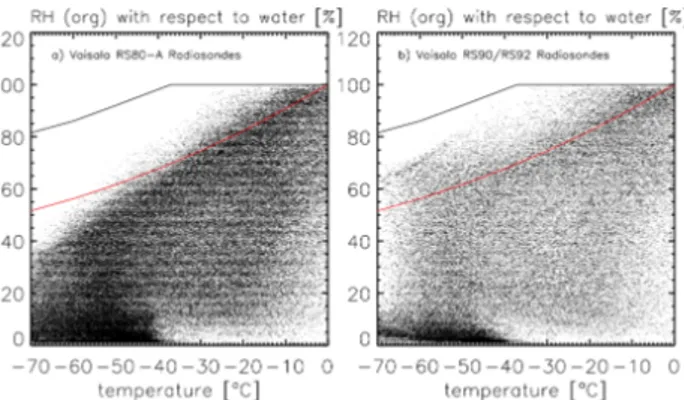
Relative humidity obtained from radiosondes is traditionally viewed with suspicion below −40◦C. The newer generations of radiosondes perform better in the upper troposphere than their predecessors, though they still do not perform well in the stratosphere. Figure 1 depicts the original RH measure-ments obtained at Ny- ˚Alesund by the different radiosondes. The data strongly suggest measured humidity values being far too low with the RS80-A relative humidity measurements rarely reaching ice saturation at temperatures below −40◦C. But the existence of high supersaturation with respect to ice in the middle and upper troposphere is well documented (e.g., Ovarlez et al., 2002). When considering data derived from the newer radiosondes RS90 and RS92, supersatura-tion with respect to ice is clearly reached much more often over the same range of ambient temperatures. These results are not surprising since Miloshevich et al. (2001) showed a strong bias towards low humidity values at low temperatures for the Vaisala RS80-A radiosonde. He reported correction factors for the relative humidity of 1.3 at −35◦C, and 2.4 at −70◦C. As a result, we used well-established algorithms to correct the available relative humidity data at Ny- ˚Alesund as described in the following section. A period in which the RS80-A and RS90 sondes were launched together on the same balloon allow us to validate the correction and to esti-mate the most probably range of actual relative humidity.
3.2 RH data correction procedure
Although the Vaisala RH sensors are all subject to the same general source of measurement errors, the magnitude of error depends strongly on the sensor type. Experiments have been performed to understand and quantify the source of RH mea-surement errors in RS80-A and RS90 sensors (Miloshevich et al., 2001, 2004, 2006; Wang et al., 2002). These authors describe different sources of error for RH measurements and present empirically based methods to correct archived ra-diosonde data and quantify the importance of various errors in the data. We followed their approach to correct the three main types of errors presented in their papers, the contami-nation/calibration error, the temperature dependence, and the time lag effect.
Firstly the contamination error and two errors resulting from the sensor calibration process were addressed. The RS80-A calibration function relating capacitance to RH at a fixed temperature, has limitations. Wang et al. (2002 here-inafter referred to as W02) proposed a correction equation (their equation 4.6-A) in the form of a fourth order polyno-mial to correct for this error. The contamination error was taken into account using W02 (their formula 4.1-A) for all RS80-A sondes until June 2000, when Vaisala fixed the
con-Figure 1. Data set of RH measurements from Ny-Ålesund radiosondes. a) for RS80
Fig. 1. Data set of RH measurements from Ny- ˚Alesund radioson-des. (a) for RS80-A radiosondes between mid October 1991 and mid July 2002 (b) for RS90/RS92 radiosondes between mid July 2002 and December 2006. Analysis based on 200-m-profiles. Red solid curve is ice saturation (Buck 1981) and black solid line is the homogenous ice nucleation level from Koop et al. (2000).
tamination problem with a sealed sensor cap. As no infor-mation about the age of an individual radiosonde was avail-able, in this study we used a constant age of one year when calculating the age-dependence portion of the contamination correction. Radiosondes are normally not stored for more than one year at the station; therefore, our correction in this case will be an upper limit for this error which is small for the RS80-A series (see for details Wang et al., 2002). No contamination correction has been determined for the RS90, because the error is thought to be much smaller due to the replacement of Styrofoam in the radiosonde construction by cardboard (Miloshevich et al., 2004).
Secondly the data was corrected for the temperature de-pendent error by applying formula 4.5 from W02. The temperature-dependent error is not a limitation of the sensor but is a consequence of the data processing algorithm. The temperature-dependent coefficients delivered with the RS80-A assume a linear dependence on temperature, whereas ap-proximation to the actual sensor dependence is significantly non-linear. The linear approximation leads to a temperature-dependent error that increases substantially for temperatures below −30◦C (Miloshevich et al., 2001).
Finally, the time lag error was corrected using the algo-rithm developed by Miloshevich et al. (2004 hereinafter re-ferred to as M04). At low temperatures, the sensor is unable to respond quickly to changes in the ambient RH, leading to a time-lag error that smoothes the RH profile and decreases the scale of details that are resolved. By using the sensor time constant as a function of temperature, the underlying structure of the RH profile can be partly recovered.
The magnitude and sign of the correction varies according to the vertical humidity and temperature structure of a given profile, because it is sensitive to the local humidity gradi-ent as well as to the temperature. RS90 data was also cor-rected for mean calibration errors following the approach of
1 2 3 4 5 6 7 8 9 10 H e ig h t [km ] -20 -10 0 10 20 Absolute difference [%RH units]
-20 -15 -10 -5 0 5 10 Ab so lu te d if fe re n ce [ % R H u n it s ] -60 -50 -40 -30 -20 -10 0 Temperature [oC] RS80org-RS90cor RS80cor-RS90cor RS80M01-RS90cor RS80org-RS90cor RS80cor-RS90cor RS80M01-RS90cor
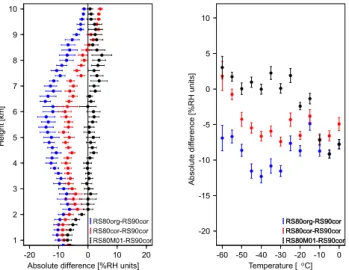
Figure 2. Absolute humidity difference (%RH) between corresponding RS80-A and RS90
Fig. 2. Absolute humidity difference (%RH) between
correspond-ing RS80-A and RS90 measurements shown as function of height
(a) and temperature (b) for 12 tandem flights in March and April
2000 performed on the same balloon. Data points are the mean in 200 m height bins or 5◦C temperature bins including the standard error of the mean. Plotted are the difference between the original RS80-A data and corrected RS90 data as described in section 3.2 (blue), the difference between the corrected RS80-A and corrected RS90 data (red) as well as the difference between the RS80-A using the approach of M01 and RS90 corrected (black).
Miloshevich et al. (2006 hereinafter referred to as M06). This method involves time lag correction plus an empirical cal-ibration correction that removes mean bias error relative to simultaneous measurements by the new hygrometer (V¨omel et al., 2007). As this comparison refers to nighttime sound-ings, it might be expected that daytime soundings in the sum-mer will exhibit a solar dry bias, particularly those taken with a RS90. So our correction process is to apply correc-tions for contamination and calibration (W02), temperature dependence (W02) and time lag error (M04) to RS80-A data while only the time lag (W04) and calibration (M06) cor-rections are applied to data from the RS90 and RS92 sonde data. Miloshevich et al. (2001) presented another correc-tion, which is a separate statistical approach that implicitly includes all sources of measurements error by removing the RS80-A mean bias relative to the NOAA hygrometer as a function of temperature. The formula used by Miloshevich et al. (2001, hereinafter referred to as M01) is a fourth-order polynomial and was applied separately to the RS80-A data for comparison purposes.
3.3 Comparison analysis
The correction algorithms have been evaluated by compar-ing 12 RH profiles measured simultaneously by RS80-A and RS90 radiosondes in March and April 2000. The profiles were corrected as described in the previous section. We have also evaluated the statistical correction produced by M01 for
0 10 20 30 40 50 60 70 80 90 100 R H [% ] (R S 9 0 ) 0 10 20 30 40 50 60 70 80 90 100 RH[%] (RS80) RS80org/RS90cor RS80cor/RS90cor RS90cor = 1.4*RS80org + 1.9 RS90cor = 1.1*RS80cor - 0.4
Figure 3. Correlation RS80-A and RS90 for temperatures below -40°C before and after Fig. 3. Correlation RS80-A and RS90 for temperatures below
−40◦C before and after correction as described in Sect. 3.2 for the 12 tandem flights performed in March and April 2000 at
Ny-˚
Alesund on the same balloon.
the RS80-A profiles. We used the corrected RS90 as refer-ence for the comparison. Figure 2 shows the differrefer-ence in rel-ative humidity (%RH) for the RS80-A and RS90 instruments as a function of altitude and temperature. The mean abso-lute difference between the original RS80-A data and the cor-rected RS90 data can be as large as 15% (Fig. 2a). Figure 2b shows that the difference is generally larger at lower temper-atures. After correcting for the contamination, time-lag and time dependent errors the mean RH difference is substan-tially reduced for temperatures above −50◦C (Fig. 2b). RH from the corrected RS80-A is generally around 5% RH lower in the lower and mid troposphere and 5% moister than RS90 in the upper troposphere (Fig. 2a). The statistical correction using M01 for the RS80-A reduces the difference for the tem-perature range between −10◦C to −40◦C but produces too high values at lower temperatures. This is probably due to the fact that the correction (M01) was derived from daytime RS80-A/NOAA comparisons when the sensor cap had been removed thus increasing the solar radiation error.
Figure 3 shows a comparison of RH for all 12 com-bined flights from the RS80-A and RS90 for each altitude at which the reported temperature was less than −40◦C. Above −40◦C, the influence of the correction is small (not depicted here). It is clear that the corrections substantially reduce the bias between the two sensors and allows us to estimate corrected RH typically within 10% of the newer RS90 ra-diosonde. As we like to account for all the corrections and errors, we performed the following analysis for 200 m aver-aged data.
0 1 2 3 4 5 6 7 8 9 10 11 a lt it u d e [ km ]
month of the year
Jan Feb Mar Apr May Jun Jul Aug Sep Oct Nov DecDec
0 10 20 30 40 50 60 70 8090100 RH [%] 0 1 2 3 4 5 6 7 8 9 10 11 a lt it u d e [ k m ]
month of the year
Jan Feb Mar Apr May Jun Jul Aug Sep Oct Nov DecDec
0 10 20 30 40 50 6070 8090100 RHi [%]
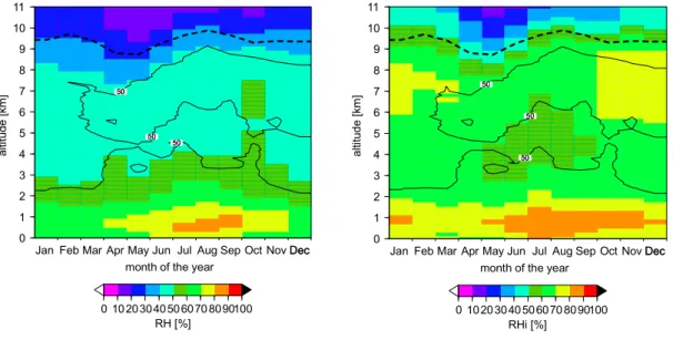
Figure 4. Monthly mean of RH (left panel) and RHi (right panel). The 50% coefficient of
Fig. 4. Monthly mean of RH (left panel) and RHi (right panel). The 50% coefficient of variation (CV) is denoted by the solid black line and
the mean tropopause height is shown using a dashed line.
4 Results and discussion
4.1 Mean relative humidity obtained from radiosonde data
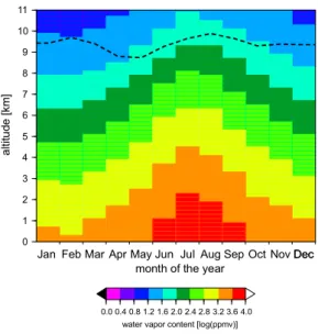
In this section, an overview is given of the statistical proper-ties of the entire corrected RH data set. The principle results and features of the whole data set are the same as those in the corresponding data subsets (RS80-A and RS90/RS92). Fig-ure 4 illustrates the corrected and monthly averaged RH and RHi (RH with respect to ice) values as a function of altitude. It also indicates where the 50% coefficient of variation (CV) is exceeded. The CV measures the relative scatter in data with respect to the mean and is a measure of the variance of the data. The higher the percentage the more variable the data distribution is. Below 2 km we found CV of less than 20% while the greatest variation is found at higher altitudes. The CV of 50% almost follows the mean tropopause height. There is also a region in the free troposphere that is charac-terised by high variability from June to September. Below 1 km the RH measurements reached their maximum mean averaged values in August of ∼80% RH compared to val-ues of ∼64% RH in February and March; however, mean RHi shows a well pronounced vertical structure in the mid-dle and upper troposphere and indicates a strong seasonal behaviour. Such seasonal behaviour is also reported from ra-diosondes and satellite data from Antarctica (Gettelman et al., 2006). Figure 5 depicts the derived monthly mean wa-ter vapour content – as obtained by the radiosondes – as a function of altitude. There is a clear seasonal variation with higher mean water vapour contents in summer than in winter. If we take, for example, a mean water vapour content in the altitude range from 2 to 8 km, the value in January is about 80% less than in July.
Table 1. Monthly mean frequency of occurrence of 200 m
ice-supersaturation layers for different RHi thresholds. Profiles anal-ysed between 0 and 11 km. Standard deviation represents the inter-annual variation.
200 m layers – RHi greater than 90% RHi 100% RHi 110% RHi Jan 27% (±9) 18% (±8) 9% (±5) Feb 26% (±6) 17% (±6) 9% (±4) March 27% (±7) 16% (±6) 8% (± 3) April 22% (±8) 12% (±5) 4% (±2) May 19% (±7) 9% (±4) 2% (±2) June 18% (±8) 7% (±4) 2% (±2) July 17% (±7) 7% (±3) 2% (±1) Aug 19% (±7) 8% (±5) 3% (±2) Sep 24% (±8) 13% (±5) 5% (±3) Oct 31% (±11) 20% (±9) 9% (±5) Nov 30% (±11) 21% (±9) 10% (±6) Dec 28% (±10) 19% (±8) 10% (±5)
4.2 Frequency of ice supersaturation layers
Here we present an analysis of the occurrence of humid lay-ers where the RH reached suplay-ersaturation with respect to ice (RHi is greater than 100%). The ice-supersaturation lay-ers can be either potential laylay-ers for ice-suplay-ersaturated re-gions (clear air) or cirrus clouds. Based on our data av-eraging, in the following section, a so-called layer corre-sponds to 200 m. Given the measurement uncertainty (see results of Sect. 3.3), we consider any altitude at which the
0 1 2 3 4 5 6 7 8 9 10 11 a lt it u d e [ km ]
month of the year
Jan Feb Mar Apr May Jun Jul Aug Sep Oct Nov DecDec
0.0 0.4 0.8 1.2 1.6 2.0 2.4 2.8 3.2 3.6 4.0 water vapor content [log(ppmv)]
Figure 5: Monthly mean of water vapour content. Dashed line represents the mFig. 5. Monthly mean of water vapour content. Dashed line rep-resents the mean tropopause height determined using the WMO’s definition of the tropopause (WMO, 1996).
ice-supersaturation for RHi exceeds 100% (±10%) between 0 and 11 km to be saturated. Table 1 summarises the mean monthly percentage of supersaturated layers. The lower and upper limits take into account uncertainties in the measure-ments as described in Sect. 3.2. The standard deviation representing the inter-annual variation is also given as an indicator of the variability within the data. As expected, the use of different RHi thresholds changes the frequency of occurrence of ice-supersaturation layers but not the gen-eral temporal or spatial evolution. This gives us the confi-dence to restrict the further analysis to RHi layers greater than 100%. During the summer (June–September), the fre-quency of occurrence is approximately half that of the rest of the year. Ice-supersaturation is most frequent in winter (October–February; 19% of all 200 m layers up to 11 km), less frequent in spring (March–May; 12%) and summer (June–September; 9%).
Overall, around 15% of all 200 m layers up to 2 km above the tropopause height showed supersaturation with respect to ice (RHi>100%). More than 50% of the profiles contain-ing supersaturation layers showed more than one layer where RHi exceeds 100%. In Fig. 6 we analysed the occurrence of these layers with respect to the month of the year and alti-tude. The frequency of occurrence of the observed supersat-urated layers follows a clear annual cycle. Figure 6 shows that saturation with respect to ice during autumn/winter time (October–February) is frequent in a broad upper tropospheric layer between ∼4 and 10 km. In summer, the layers saturated with respect to ice are less frequent and occur at higher alti-tudes generally between 7 and 9 km. A t-test was highly sig-nificant at p<10−3for the seasonal shift. Figure 6 also indi-cates that the ice-supersaturation tends to consistently track
0 1 2 3 4 5 6 7 8 9 10 11 a lt it u d e [ km ]
month of the year
Jan Feb Mar Apr May Jun Jul Aug Sep Oct Nov DecDec
0 10 20 30 40 50 frequency of occurrence [%]
Figure 6. Monthly mean frequency of occurrence of ice-supersaturation layers. The frequency
Fig. 6. Monthly mean frequency of occurrence of
ice-supersaturation layers. The frequency of occurrence is defined here as the number of observations in a 200 m altitude range where RH with respect to ice is greater than 100% divided by the total number of observations for this altitude range. Dashed line represents the mean tropopause height determined using the WMO’s definition of the tropopause (WMO, 1996).
the tropopause height. Around one third of the supersatu-rated layers are within 1 km of the tropopause for tempera-tures below −35◦C.
4.3 Comparison to other studies of radiosonde data
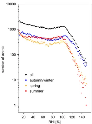
Observations from radiosondes suggest that the distribution of RHi in ice-supersaturated layers follows an almost expo-nential distribution, indicating that the underlying processes, which cause this functional dependence, act in a statisti-cally independent manner. This was reported in the analy-sis of humidity data from MOZAIC (Gierens et al., 1999), MLS (Spichtinger et al., 2002), radiosondes at Lindenberg (Spichtinger et al., 2003), and TOVS data (Gierens et al., 2004). We find that the Ny- ˚Alesund RHi data in excess of 100% also follow an exponential distribution for the up-per troposphere. In Fig. 7, we depict the (non-normalized) frequency distributions of the relative humidity over ice N(RHi). While not overly sensitive to the altitude range, we have limited the altitude range above 4 km height to be consistent with earlier studies. However, the features re-main the same if we include the entire altitude range. In addition, since we observe that supersaturated layers show a strong seasonal behaviour (Fig. 7), we determined the fre-quency distribution for three time periods (autumn/winter = October–February, spring = March–May and summer = June–September). These subsets were chosen to cover the dark part of the year, and to follow other studies, which showed large changes in the aerosol characteristics for the
Table 2. Exponents b for the frequency distribution law ln[N (k)]=a−b ∗ k as obtained from straight fitting to the distribution of relative
humidity with respect to ice, RHi, shown in Fig. 7. The standard deviation σbfor the determined values b is given in brackets. Values have been multiplied by 100 for easier reading. For altitudes above 4 km, the data base was divided into two sets, one where the humidity was at and above ice saturation (ice-supersaturation layers – ISS) and one were the humidity was below ice saturation (non ice-supersaturation layers – Non-ISS). Analysis based on 200-m-profiles. Autumn/winter (October–February); spring (March–May) and summer (June–September). We note that a performed Kolmogorov-Smirnov test showed a significant differences between spring (summer) and winter distribution but no significant difference between spring and summer distribution.
Fit range Temperature [◦C] Water vapour content [ppmv]
Non – ISS ISS Non – ISS ISS
110-150 20-80 mean 98%/2% mean 98%/2% mean 98%/2% mean 98%/2% ratio
Total 7.9 (0.1) 0.8 (0.0) −44 (13) −16/−66 −47 (12) −22/−68 237(414) 1638/9 333 (455) 1753/19 1.4 Autumn/Winter 8.8 (0.2) 1.1 (0.1) −49 (11) −25/−67 −50 (12) −26/−69 110 (196) 731/8 236 (298) 1178/17 2.1 Spring 7.0 (0.2) 1.1 (0.0) −46 (11) −22/−66 −47 (11) −25/−69 154 (245) 932/8 279 (307) 1230/16 1.8 Summer 12.0 (0.6) 0.4 (0.0) −37 (12) −13/−56 −40 (12) −17/−59 415(569) 2247/13 600 (663) 2591/58 1.4
Arctic troposphere between May and June (Str¨om et al., 2003a; Treffeisen et al., 2006). The single RHi values are binned into 150 1% wide classes (numbered from 0–149), where the last class (149) contains all data with RHi≥149%. The seasonal curves show similar behaviour (Fig. 7). Each curve is relatively smooth below 100% RHi but reaches a small maximum near 100%. Gierens et al. (2004) interpreted the existence of the local maximum, or bulge, around 100% RHi to be a product of cloud processes. Above 100%, the fre-quency of occurrence of ice-supersaturation levels decreases exponentially in all seasons. The steepness of the exponen-tial curve and location of the maximum, show seasonal de-pendence (Fig. 7). All distributions follow the same struc-ture, approximately uniform below ice saturation and de-creasing geometrically above (i.e. with the probability den-sity function PRHi(k)=qk(1−q); kε{0, 1, 2, . . .} as described
by Gierens (1999)). The exponents b=− ln q for distributions RHi have been computed for the range 20%≤RHi≤80% and 110%≤RHi≤150%, respectively, using a straight line fit to the function ln(N (k))=a−b ∗ k (Table 2). For the super-saturated part the exponents range from 0.079 for all data to 0.12 in summer. The result of the previous subsection can be used to infer the mean ice-supersaturation know-ing that the expected value of a modified geometric distri-bution is q/(1−q)=e−b/(1−e−b), therewith the mean ice-supersaturation above 4 km altitude amounts to 12% on av-erage, with seasonal variations in winter of 11%, in spring of 14% and summer of 8%. Recent studies indicate that homo-geneous freezing requires supersaturation around 145% (e.g. Haag et al., 2003, and Str¨om et al., 2003b).
These results may be compared with those of Spichtinger et al. (2003), who applied a similar analysis to one year’s radiosonde data from Lindenberg, and observed a much steeper exponent value of 0.21. Also relevant for the present study are results of Gierens et al. (1999), based on three years of data obtained from MOZAIC (b=0.058), and from
1 1 10 100 1000 10000 n u mb e r o f e v e n ts 20 40 60 80 100 120 140 RHi [%]
Figure 7. Frequency distribution (per 1% RHi bins) of relative humidity with respecFig. 7. Frequency distribution (per 1% RHi bins) of relative humid-ity with respect to ice (RHi), for data above 4 km height for the fol-lowing time periods: all (black); autumn/winter (October–February; blue), spring (March–May; orange) and summer (June–September; red).
Spichtinger et al. (2002) who obtained b=0.051 from MSL data. As the authors do not separate data into seasons, our value for the entire data set above 4 km altitude of b=0.079 agrees rather well with these published results; however, their results are averaged over large geographical regions and are not immediately comparable with a single station,
as Ny- ˚Alesund. We note that the summer distribution is dif-ferent from the other seasons. A similar seasonal pattern in RHi distribution was reported by Vaughan et al. (2005) for mid-latitude upper tropospheric radiosonde data from Wales. Due to the measurement uncertainty of ±10% it is not pos-sible to distinguish whether the local maxima of the distri-butions are located above or below ice saturation (Fig. 7). We also note that the observed bulge is less pronounced in spring compared to the other periods. It is possible that dy-namic processes suppress the build-up of high supersatura-tion in summer or that differences in cloud processes create the observed seasonal differences.
For altitudes above 4 km, data was divided into two data sets, one where the humidity was at or above ice satura-tion and one where the humidity was below ice saturasatura-tion. For these subsets we calculated the mean temperature and 98% (2%) percentile values (see Table 2). Mean temper-atures in ice-supersaturated layers tend to be lower (3 K) than in non supersaturated layers. The colder air in ice-supersaturated layers suggests that uplifting of airmasses is one major source of ice-supersaturation layers as discussed by Gierens et al. (1999) in connection to MOZAIC data. The flight data is different from the radiosonde data as air-craft measurements are made on a specific pressure level and the sounding data provides information in the vertical. Another possible origin of ice-supersaturation in the tro-posphere might be advection of moisture leading to vari-ations in absolute water vapour content. We have deter-mined mean and standard deviation of the water vapour con-tent. The results are displayed in Table 2. The standard deviations are comparable, or larger than the mean values. The derived mean values show that water vapour content is considerably larger in ice-supersaturation layers than in non ice-supersaturation layers. The lowest values of water vapour content for supersaturation layers and non ice-supersaturation layers are reached in autumn/winter. The ra-tio between the two layer types is highest in autumn/winter with 2.1 and lowest in summer with 1.4. The general evo-lution of the water vapour content in the Arctic atmosphere over Ny- ˚Alesund can also be seen in Fig. 5. Therefore, we believe that moisture advection plays an important role in the formation of ice-supersaturated regions.
4.4 Vertical and seasonal variation extent of ice-supersaturation layers
The profiles of RH measurements allow us to investigate the vertical extent of the ice-supersaturation layers. This is related to the potential thickness of clouds, even though a large amount of the higher supersaturations probably occurs in clear air. Of special interest is the cloud’s ability to re-flect sunlight and thus influence the radiative balance and this depends on the cloud’s thickness. Spichtinger et al. (2004) discussed the differences in the bulge signature in frequency distributions of the relative humidity over ice as possibly
re-lated to different cloud thickness. To be able to compare our results to Spichtinger et al. (2004), we restrict our data base to layers above 4 km height.
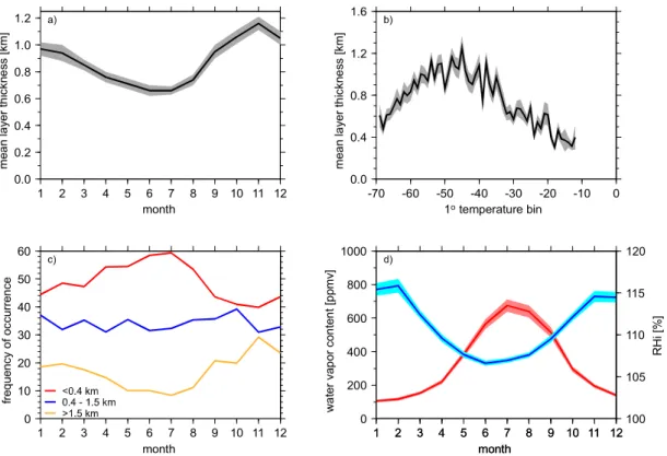
In order to derive the vertical extent of ice-supersaturation for each single sounding profile, we combined all adjacent 200 m ice-supersaturation layers into one single layer. Each such layer is then characterised by the altitude of its lower and upper boundary, its depth (layer thickness) as well as its mid-layer temperature. The mean layer thickness reaches its minimum of ∼0.7 km in summer (Fig. 8a) increasing by ∼50% in winter. Figure 8b shows the mean layer thickness as a function of mid layer temperature. The maximum layer thickness is reached at temperatures around −45◦C. Indeed, approximately 70% of the adjacent ice-supersaturated lay-ers have a mid-layer temperature below −40◦C. Lidar mea-surements by Goldfarb et al. (2001) in France and Cadet et al. (2003) in Reunion determined an average cloud layer thickness for cirrus of approximately 1.4 km±1.3 and a markedly thinner cloud layer thickness for subvisible clouds between 0.4 and 0.8 km. In light of this, we were interested in how the thickness of the ice-supersaturation layers devel-ops from month to month at our site. To do this, we divided the layer thickness in different ranges as depicted in Fig. 8c. One interesting difference is the summertime increase of thin layers with a thickness of up to 400 m and the decrease of layers thicker than 1.5 km. The number of layers between 0.4 and 1.5 km is relatively constant during the year. With our data set, we are not able to determine what causes these seasonal differences. Figure 8d demonstrates the evolution of the monthly averaged RHi obtained in the ice-supersaturation layers and of the corresponding water vapour content. The shape of the two curves strongly suggests an anticorrelation between the parameters.
A method to get more detailed information on the verti-cal extent of these layers was described by Spichtinger et al. (2003). Using a statistical approach described by Berton (2000) to analyse ice-supersaturation layers, they showed that the thickness of ice-supersaturation layers over Linden-berg followed a Weibull distribution with different slopes for shallow and thicker layers. They also determined that the transition between the two regimes occurred around 1 km thickness. We performed a similar analysis for our data set and found the transition occurred at a thickness around 2 km. The deeper layers are most likely cirrus clouds. The slope of the line in this part is 0.9. For visible cirrus, the corresponding shape parameter is around 1 (Berton, 2000; Spichtinger et al., 2003). Layers less thick than 2 km prob-ably contain data from true ice-supersaturation layers and perhaps sub-visible cirrus. The slope for these thinner lay-ers is around 0.5. Almost 90% of the laylay-ers are thinner than 2 km. As not only layer thickness but also the avail-able cloud water content is important for determining cloud characteristics, this can only act as a first step in the analysis of the ice-supersaturation layers. This needs further investi-gation, especially coupling the RHi data with remote sensing
0.0 0.2 0.4 0.6 0.8 1.0 1.2 me a n l a y e r th ic kn e s s [k m ] 1 2 3 4 5 6 7 8 9 10 11 12 month 0.0 0.4 0.8 1.2 1.6 me a n l a y e r th ic kn e s s [k m ] -70 -60 -50 -40 -30 -20 -10 0 1o temperature bin 0 10 20 30 40 50 60 fr e q u e n c y o f o c cu rr e n ce 1 2 3 4 5 6 7 8 9 10 11 12 month 0 200 400 600 800 1000 w a te r va p o r co n te n t [p p m v ] 1 2 3 4 5 6 7 8 9 10 11 12 month 100 105 110 115 120 R H i [% ] 1 2 3 4 5 6 7 8 9 10 11 12 month
Figure 8. This figures show different statistics on all determined supersaturation layers above
Fig. 8. This figures show different statistics on all determined supersaturation layers above 4 km height: (a) Monthly mean of the amount
of the layer thickness and the standard deviation of the mean; (b) mean layer thickness and standard deviation of the mean as a function of 1◦temperature bins based on the mid-layer temperature (c) monthly occurrence of different thickness ranges; (d) Monthly averaged water vapour content (red line) and RHi of adjacent ice- supersaturation layers (blue line).
data obtained from Ny- ˚Alesund, such as micropulse lidar or ceilometer in order to get more insight in the layer character-istics.
4.5 Combining ice-supersaturation layers and subvisible clouds detected by SAGE II
We have studied the relation between ice-supersaturated lay-ers and subvisible clouds (SVC) by looking at data from the Stratospheric Aerosol and Gas Experiment II (SAGE II) satellite. Gierens et al. (2000) showed an association be-tween ice-saturated regions with SAGE II SVC. SAGE II aerosol products provide the opportunity of investigating the occurrence of SVC in the Arctic on a statistical basis. Ide-ally one would like to correlate the occurrence of SVC and the existence of ice-supersaturation on a case by case ba-sis. Unfortunately, this is not practicable with the SAGE data. Single events cannot be used here because it is rather rare that SAGE measurements and the radio soundings are concurrent. Thus, we decided to compare the data on a monthly basis for all data available north of 60◦ and aver-aged the sounding results to the altitude resolution of SAGE II. The approach of analysing monthly averaged SAGE data has already been used to derive principal aerosol characteris-tics in the upper Arctic troposphere (Treffeisen et al., 2006).
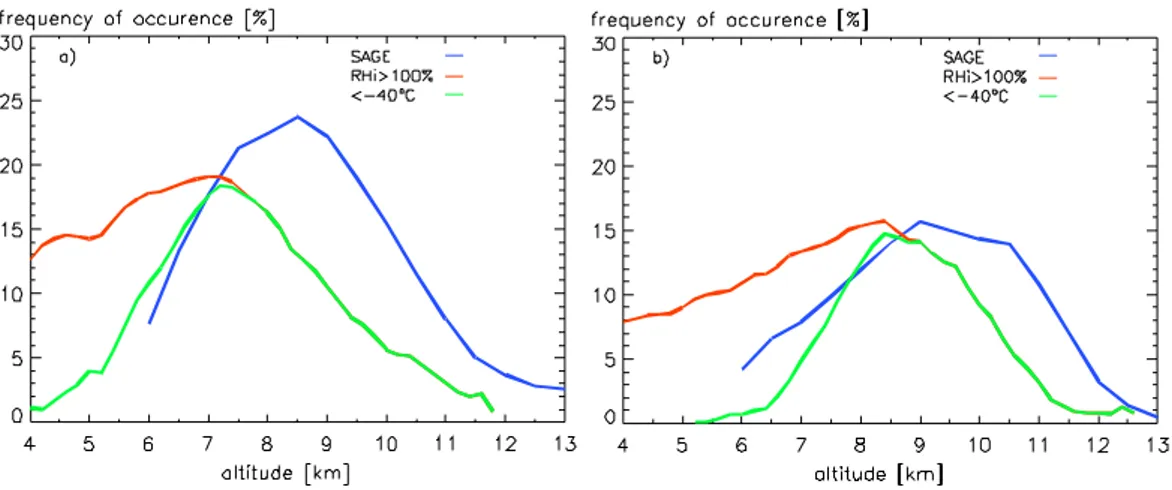
The SVC from SAGE II are most often detected around the tropopause height. Approximately 80% of the detected SVC are located within 3 km of the tropopause. The vertical distri-bution of SVC detected by SAGE is presented for the spring and summer in Fig. 9, together with the frequency of occur-rence of ice-supersaturated layers. The peak of occuroccur-rence of SVC is pronounced in both periods showing a maximum of about 24% in March to April compared to 15% in summer, whereas the location of the maximum is shifted only slightly from 8.5 km in spring to 9 km in summer for the SAGE II measurements. The general similarity between the altitude distributions is very good. Where the frequency of occur-rence of ice-supersaturation is high, the occuroccur-rence of SVC is also high, and visa versa. Restricting ice-supersaturation layers to temperatures below −40◦C increases the agreement for the lower altitude ranges. These results suggest that a sig-nificant fraction of the sonde-observed ice supersaturation layers are most probably attributable to subvisible clouds. A statistical analysis of cloud occurrence performed on 11 months of data from Ny- ˚Alesund showed 5% of clouds to be in the altitude range from 6 to 12 km on average and thicker clouds in summer than in winter time (Shiobara et. al, 2003). Future studies should directly compare cloud measurements with the obtained ice-supersaturation layers.
Figure 9. Mean frequency distribution of all ice-supersaturation layers obtained by the
Fig. 9. Mean frequency distribution of all ice-supersaturation layers obtained by the radiosondes (red line) and ice-supersaturation layers
when the temperature is below −40◦C (green line). As well depicted the frequency of occurrence of SVC vs. altitude, as obtained from SAGE II satellite measurements for the latitude band 60◦N–80◦N; (a) calculated for March, April and May; (b) calculated for June, July, August and September.
Considering the large temporal and vertical variability, the agreement between SAGE II SVC and ice-supersaturated layers from radiosondes is very good. The differences in lo-cation and height of the maximum in spring (Fig. 9) might be due to processes that decouple SVC from ice-supersaturation layers and ice-supersaturation alone does not produce a unique spectral signature in the SAGE II data. Differences can also result from the large spatial coverage of the SAGE II satellite, compared to the point measurement with the ra-diosonde, and the quality of the SAGE II cloud measure-ments, which can be affected by aerosol-cloud mixture, frac-tional cloud coverage of the viewing window and fracfrac-tional cloud distribution along the viewing window and viewing path (Wang et al., 1995).
5 Conclusions
We analysed a unique high latitude data set of tropospheric humidity profiles measured with standard radiosondes at
Ny-˚
Alesund (78◦55′N 11◦52′E) during the period from 1991 to 2006. The sounding data were corrected using previ-ously published algorithms. Despite the extensive correc-tions, there is still an uncertainty associated with the diffi-culties of radiosonde RH measurements at low temperatures and we were not able to lower the realistic error below ±10% RH. The corrected data were used to determine the main characteristics of the tropospheric relative humidity distribu-tion in the vicinity of Ny- ˚Alesund. It is clear from the ra-diosondes that supersaturation with respect to ice is observed throughout the year. It indicates that supersaturation over ice is a frequent condition in the Arctic middle and upper tro-posphere, particularly during autumn/winter. The frequency of occurrence of ice-supersaturation levels decreases expo-nentially with the magnitude of ice-supersaturation and is in
good agreement with other studies. The mean frequency of occurrence of ice-supersaturation layers follows a clear sea-sonal variation with a value of 19% in winter, 12% in spring and 9% in summer. The ice-supersaturation occurs mostly in a broad band between 6 and 9 km in winter and undergoes a shifting towards higher altitudes in summer. The altitude dis-tribution of ice-supersatured layers over Ny- ˚Alesund is gen-erally similar to that of subvisible clouds from the SAGE II experiment and thus confirms the existence of SVC in the Arctic atmosphere. While one might expect the soundings to observe different frequencies from SAGE II, owing to the different sampling volumes (the SAGE II instrument samples horizontal distances of ∼200 km), our results show that there is a strong positive correlation between both independent ob-servations, which indicates that ice-supersaturated layers as-sociated with sub-visible cirrus are likely to be a wide spread phenomenon over the Arctic. This brings attention to the im-portant subject of the SVC influence on the radiative budget in the Arctic, which is currently unexplored.
This study focused on a general first description of the ice-supersaturation layers over Ny- ˚Alesund. Continuation of this work will attempt to compare these results directly to ground-based Lidar systems and CALIPSO satellite data. This can give us information on the internal structure of the layers and will help us to understand cloud formation pro-cesses.
Acknowledgements. We give thanks to the following: For financial support to International Meteorological Institute (IMI), Swedish Research Council, Swedish Polar Secretariat and Alfred Wegener Institute, who made this study possible. We also like to say thank you to H. Deckelmann, who prepared the final picture layout. Edited by: H. Wernli
References
Baker, M. B.: Cloud microphysics and climate, Science, 276, 1072– 1078, 1997.
Bakan, S., Betancor, M., Gayler, V., and Grassl, H.: Contrail fre-quency over Europe from NOAA satellite images, Ann. Geo-phys., 12, 962–968, 1994,
http://www.ann-geophys.net/12/962/1994/.
Bates, J. J. and Jackson, D. J.: Trends in upper-tropospheric humid-ity, Geophys. Res. Lett., 28, 1695–1698, 2001.
Berton, R. P. H.: Statistical distribution of water content and sizes for clouds above Europe, Ann. Geophys., 18, 385–397, 2000, http://www.ann-geophys.net/18/385/2000/.
Buck, A.: New equation for computing vapor pressure and enhance-ment factor, J. Appl. Meteorol., 20, 1527–1532, 1981.
Cadet, B., Goldfarb, L., Faduilhe, D., Baldy, S., Giraud, V., Keck-hut, P., and R´echou, A.: A sub-tropical cirrus clouds climatology from Reunion Island (21◦S, 55◦E) lidar data set, Geophys. Res. Lett., 30(3), 1130, doi:10.1029/2002GL016342, 2003.
Elliott, W. P. and Gaffen, D. J.: On the utility of radiosonde hu-midity archives for climate studies, B. Am. Meteorol. Soc., 72, 1507–1520, 1991.
Gettelman, A., Walden, V. P., Miloshevich, L. M., Roth, W. L., and Halter, B.: Relative humidity over Antarctica from radiosondes, satellites, and a general circulation model, J. Geophys. Res., 111, D09S13, doi:10.1029/2005JD006636, 2006.
Gierens, K, Schumann, U., Helten, M., Smit, H., and Marenco, A.: A distribution law for relative humidity in the upper troposphere and lower stratosphere derived from three years of MOZAIC measurements, Ann. Geophys., 17, 1218–1226, 1999,
http://www.ann-geophys.net/17/1218/1999/.
Gierens, K., Schumann, U., Helten, M., Smit, H., and Wang, P.-H.: Ice-supersaturated regions and subvisible cirrus in the north-ern midlatitude upper troposphere, J. Geophys. Res., 105(D18), 22 743–22 754, doi:10.1029/2000JD900341, 2000.
Gierens, K., Kohlhepp, R., Spichtinger, P., and Schroedter-Homscheidt, M.: Ice supersaturation as seen from TOVS, Atmos. Chem. Phys., 4, 539–547, 2004,
http://www.atmos-chem-phys.net/4/539/2004/.
Goldfarb, L., Keckhut, P., Chanin, M.-L., and Hauchecorne, A.: Cirrus Climatological Results from Lidar Measurements at OHP (44◦N, 6◦E), Geophys. Res. Lett., 28, 1687–1690, doi:10.1029/2000GL012701, 2001.
Haag, W., K¨archer, B., Str¨om, J., Minikin, A., Lohmann, U., Ovar-lez, J., and Stohl, A.: Freezing thresholds and cirrus cloud forma-tion mechanisms inferred from in situ measurements of relative humidity, Atmos. Chem. Phys., 3, 1791–1806, 2003,
http://www.atmos-chem-phys.net/3/1791/2003/.
Kent, G. S., Winkler, D. M., Osborn, M. T., and Skeens, K. M.: A model for the separation of cloud and aerosol in SAGE II occul-tation data, J. Geophys. Res., 98, 20 725–20 735, 1993.
Koop, T., Puo, B. L., Tsias, A., and Peter, T.: Water activity as the determinant for homogeneous ice nucleation in aqueous so-lutions, Nature, 406, 611—614, 2000.
Liou, K.-N.: Influence of cirrus clouds on weather and climate pro-cesses: A global perspective, Mon. Wea. Rev., 114, 1167–1199, 1986.
Miloshevich, L. M., V¨omel, H., Paukkunen, A., Heymsfield, A. J., and Oltmans, S. J.: Characterization and Correction of Relative Humidity Measurements from Vaisala RS80-A Radiosondes at
Cold Temperatures, J. Atmos. Oceanic Technol., 18, 135–156, 2001.
Miloshevich, M., Paukkunen, A., V¨omel, H., and Oltmans, S.: De-velopment and Validation of a Time-Lag Correction for Vaisala Radiosonde Humidity Measurements, J. Atmos. Oceanic Tech-nol., 21, 1305–1327, 2004.
Miloshevich, L. M., V¨omel, H., Whiteman, D. N., Lesht, B. M., Schmidlin, F. J., and Russo, F.: Absolute accuracy of water vapor measurements from six operational radiosonde types launched during AWEX-G and implications for AIRS validation, J. Geo-phys. Res., 111, D09S10, doi:10.1029/2005JD006083, 2006. Murphy, D. M., Kelly, K. K., Tuck, A. F., Proffitt, M. H., and
Kinne, S.: Ice saturation at the tropopause observed from the ER-2 aircraft, Geophys. Res. Lett., 17(4), doi:10.10ER-29/90GL003ER-27, 1990.
Ovarlez, J., Gayet, J. F., Gierens, K., Str¨om, J., Ovarlez, H., Auriol, F., Busen, R., and Schumann, U.: Water vapour measurements inside cirrus clouds in Northern and Southern hemispheres during INCA, Geophys. Res. Lett., 29(16), 1813, doi:10.1029/2001GL014440, 2002.
Randel, D. L., Vonder Haar, T. H., Ringerud, M. A., Stephens, G. L., Greenwald, T. J., and Combs, C. L.: A New Global Water Vapor Dataset, B. Am. Meteorol. Soc., 77, 1233–1246, 1996. Schmidlin, F. J. and Ivanov, A.: Radiosonde relative humidity
sensor performance: The WMO intercomparison–Sept 1995, Preprints, 10th Symp. on Meteorological Observations and In-strumentation, Phoenix, AZ, Am. Meteorol. Soc., 68–71, 1998. Stephens, G. L., Tsay, S. C., Stackhouse, P. W., and Flatau, P. J.:
The relevance of the microphysical and radiative properties of cirrus clouds to climate and climatic feedback, J. Atmos. Sci., 47, 1742–1753, 1990.
Shiobara, M., Yabuki, M., and Kobayashi, H.: A polar cloud anal-ysis based on Micor-pulse Lidar measurements at Ny- ˚Alesund, Svalbard and Syowa, Antarctica, Phys. Chem. Earth, 28, 1205– 1212, 2003.
Spichtinger, P., Gierens, K., and Read, W.: The statistical distri-bution law of relative humidity in the global tropopause region, Meteorol. Z., 11, 83–88, 2002.
Spichtinger, P., Gierens, K., Leiterer, U., and Dier, H.: Ice super-saturation in the tropopause region over Lindenberg, Germany, Meteorol. Z., 12, 143–156, 2003.
Str¨om, J., Umeg˚ard, J., Tøseth, K., Turnved, P., Hansson, H.C., Holm´en, K., Wisman, V., Herber, A., and K¨onig-Langlo, G.: One year observation of particle size distribution and aerosol chemi-cal composition at the Zeppelin Station, Svalbard, March 2000– March 2001, J. Phys. Chem. Earth, 28, 1181–1190, 2003a. Str¨om, J., Seifert, M., K¨archer B., Ovarlez, J., Minikin, A., Gayet,
J.-F., Krejci, R., Petzold, A., Auriol, F., Busen, R., Schumann, U., Haag, W., and Hansson, H.-C.: Cirrus cloud occurrence as function of ambient relative humidity: a comparison of observa-tions from the Southern and Northern Hemisphere midlatitudes obtained during the INCA experiment, Atmos. Chem. Phys., 3, 1807–1816, 2003b.
Treffeisen, R. E., Thomason, L. W., Str¨om, J., Herber, A. B., Bur-ton, S. P., and Yamanouchi, T.: SAGE II and III aerosol extinc-tion measurements in the Arctic middle and upper troposphere., J. Geophys. Res. 111, D17203, doi:10.1029/2005JD006271, 2006.
vapour and ozone profiles in the midlatitude upper troposphere, Atmos. Chem. Phys., 5, 963–971, 2005,
http://www.atmos-chem-phys.net/5/963/2005/.
V¨omel, H., David, D., and Smith. K.: Accuracy of tropospheric and stratospheric water vapor measurements by the Cryogenic Frost point Hygrometer (CFH): Instrumental details and observations, J. Geophys. Res., 112, D08305, doi:10.1029/2006JD007224, 2007.
Wang, P. H., McCormick, M. P., Poole, L. R., Chu, W. P., Yue, G. K., Kent, G. S., and Skeens, K. M.: Tropical high cloud charac-teristics derived from SAGE II extinction measurements, Atmos. Res., 34, 53–83, 1994.
Wang, P. H., Minnis, P., and Yue, G. K.: Extinction coefficient (1 µm) properties of high altitude clouds from solar occultation measurements (1985–1990): evidence of volcanic aerosol effect, J. Geophys. Res., 100(2), 3181–3199, 1995.
Wang, P. H., Minnis, P., McCormick, M. P., Kent, G. S., and Skeens, K. M.: A 6-year climatology of cloud occurrence frequency from Stratospheric Aerosol and Gas Experiment II observations (1985–1990), J. Geophys. Res., 101, 29 407–29 429, 1996. Wang, J., Cole, H., Carlson, L., Miller, D. J., Beierle, E. R.,
Paukkunen, K., and Laine, T. K.: Corrections of Humidity Mea-surement Errors from the Vaisala RS80 Radiosonde-Application to TOGA COARE Data, J. Atmos. Oceanic Technol., 19, 981– 1002, 2002.
WMO: Measurements of upper air temperature, pressure, and hu-midity. Guide to Meteorological Instruments and Methods of Ob-servation, 6th ed., WMO I.12-1–I.12-32, 1996.
Wylie, D. P., Menzel, W. P., Woolf, H. M., and Strabala, K.: Four Years of Global Cirrus Cloud Statistics Using HIRS, J. Climate, 7, 1972–1986, 1994.