HAL Id: hal-00317678
https://hal.archives-ouvertes.fr/hal-00317678
Submitted on 3 Nov 2004
HAL is a multi-disciplinary open access
archive for the deposit and dissemination of
sci-entific research documents, whether they are
pub-lished or not. The documents may come from
teaching and research institutions in France or
abroad, or from public or private research centers.
L’archive ouverte pluridisciplinaire HAL, est
destinée au dépôt et à la diffusion de documents
scientifiques de niveau recherche, publiés ou non,
émanant des établissements d’enseignement et de
recherche français ou étrangers, des laboratoires
publics ou privés.
the equatorial and low-latitude ionosphere in the context
of the Indian tomography experiment: CRABEX
S. V. Thampi, T. K. Pant, S. Ravindran, C. V. Devasia, R. Sridharan
To cite this version:
S. V. Thampi, T. K. Pant, S. Ravindran, C. V. Devasia, R. Sridharan. Simulation studies on the
tomographic reconstruction of the equatorial and low-latitude ionosphere in the context of the Indian
tomography experiment: CRABEX. Annales Geophysicae, European Geosciences Union, 2004, 22
(10), pp.3445-3460. �hal-00317678�
SRef-ID: 1432-0576/ag/2004-22-3445 © European Geosciences Union 2004
Annales
Geophysicae
Simulation studies on the tomographic reconstruction of the
equatorial and low-latitude ionosphere in the context of the Indian
tomography experiment: CRABEX
S. V. Thampi, T. K. Pant, S. Ravindran, C. V. Devasia, and R. Sridharan
Space Physics Laboratory, Vikram Sarabhai Space Centre Trivandrum, 6 95 022, India
Received: 17 March 2004 – Revised: 9 June 2004 – Accepted: 18 June 2004 – Published: 3 November 2004
Abstract. Equatorial ionosphere poses a challenge to any
al-gorithm that is used for tomographic reconstruction because of the phenomena like the Equatorial Ionization Anomaly (EIA) and Equatorial Spread F (ESF). Any tomographic re-construction of ionospheric density distributions in the equa-torial region is not acceptable if it does not image these phe-nomena, which exhibit large spatial and temporal variabil-ity, to a reasonable accuracy. The accuracy of the recon-structed image generally depends on many factors, such as the satellite-receiver configuration, the ray path modelling, grid intersections and finally, the reconstruction algorithm. The present simulation study is performed to examine these in the context of the operational Coherent Radio Beacon Ex-periment (CRABEX) network just commenced in India. The feasibility of using this network for the studies of the equa-torial and low-latitude ionosphere over Indian longitudes has been investigated through simulations. The electron density distributions that are characteristic of EIA and ESF are fed into various simulations and the reconstructed tomograms are investigated in terms of their reproducing capabilities. It is seen that, with the present receiver chain existing from 8.5◦N to 34◦N, it would be possible to obtain accurate im-ages of EIA and the plasma bubbles. The Singular Value Decomposition (SVD) algorithm has been used for the in-version procedure in this study. As is known, by the very nature of ionospheric tomography experiments, the received data contain various kinds of errors, like the measurement and discretization errors. The sensitivity of the inversion al-gorithm, SVD in the present case, to these errors has also been investigated and quantified.
Key words. Ionospheric (equatorial ionosphere; iono-spheric irregularities; instruments and techniques)
Correspondence to: S. V. Thampi
(sudha ravindran@vssc.org)
1 Introduction
The basic idea of tomographic methods, which uses the line integral measurements through a field to reconstruct the field itself, was originated by Radon in 1917 and the first practical application seems to have been published by Bracewell (1956). Since then, this technique has been ap-plied successfully in many fields. For instance, it had a rev-olutionary impact in the field of medical imaging. Austen et al. (1988) suggested that using the total electron content (TEC), the tomography technique can also be used for the two-dimensional imaging of electron density distribution in the ionosphere.
The first experimental test of the application of tomo-graphic methods for ionospheric studies was attempted us-ing coordinated observations in Scandinavia in the year 1986 (Andreeva et al., 1990; Pryse and Kersley, 1992). Simulta-neous TEC measurements were made from two stations by receiving phase coherent signals of 150 MHz and 400 MHz transmitted from a low Earth-orbiting Navy Navigational Satellite. Despite all the limitations of the experimental ar-rangement, the tomographic image could reveal the presence of a gradual, large-scale, northward electron density gradi-ent, which was confirmed by independent measurements us-ing the EISCAT radar (Raymund et al., 1993). Subsequently, several experiments were carried out in both the United Kingdom and Scandinavia, which demonstrated the poten-tial of tomography to image large-scale ionospheric, features such as troughs in electron density found at auroral and sub-auroral latitudes (Kersley et al., 1997). Apart from these, there were tomographic experiments from other parts of the world also. The most important of them include the Rus-sian Tomography Experiments, RusRus-sian-American Tomog-raphy Experiment (RATE) and the Mid-America Comput-erized Ionospheric tomography Experiment (MACE) (An-dreeva et al., 1990, 1992; Kunitsyn and Treshchenko, 1994; Foster et al., 1994). All these experiments could bring out the shape, width, slope and depth of the main ionospheric trough very clearly. These experiments could also image the
traveling ionospheric disturbances (TIDs) and quasi-wave structures which usually appear in the perturbed ionosphere. It has been unambiguously established now that the tomo-graphic techniques are very effective and useful in investi-gating the large-scale structures over low and equatorial lati-tudes, for example, equatorial ionization anomaly (EIA) (An-dreeva et al., 2000). The first network of six receivers from 14.6◦N to 31.3◦N (geographic latitudes) along the 121◦E meridian, namely the Low latitude Ionospheric Tomography Network (LITN), has provided important information about the motion of the anomaly crest of the EIA (Yeh et al., 1994, 2001), the structure and symmetry of its core (Andreeva et al., 2000) and the low-latitude ionospheric response to mag-netic storms (Ji-Sheng et al., 2000). However, questions re-garding the development of the anomaly during the course of the day, and its relationship with other ionospheric pro-cesses, like the Equatorial electrojet and equatorial spread F, calls for further systematic investigations.
The Indian Coherent Radio Beacon Experiment (CRABEX) has been just initiated mainly to address the aforementioned questions regarding the large-scale processes over equatorial and low latitudes. This ex-periment consists of six radio receivers stationed at Trivandrum (8.5◦N, 77◦E), Bangalore (13◦N, 77.6◦E), Hy-derabad (17.3◦N, 78.3◦E), Bhopal (23.2◦N, 77.2◦E), Delhi (28.8◦N, 77.2◦E), and Hanle (34◦N, 78◦E) that are capable of receiving the 150 and 400 MHz beacon transmissions from the Low Earth Orbiting Satellites (LEOS). This chain is unique as it covers the crest and trough regions of the EIA latitudinally, and goes well beyond the anomaly region. Thus, the data obtained using this chain will help in understanding the temporal and spatial evolution of equatorial and low-latitude ionospheric phenomena like EIA and ESF, and their interrelationships. For example, the degree of variability of the EIA, which is otherwise quite difficult to be monitored completely, can be understood by the tomographic methods. The maximum E×B drift, the location of the EIA crest and its intensity which are known to be intricately connected to the generation of equatorial bubbles, as well as bottomside spread F (Whalen, 2001), can be investigated in detail using the tomograms.
The measured parameter in most of the ionospheric to-mography experiments worldwide is the relative phase of 150 MHz signal with respect to that of 400 MHz, both trans-mitted coherently from a satellite borne-beacon and received on ground. The differential phase is related to the slant elec-tron content along any ray as
8 = CD×ST EC, (1)
where 8 is measured in radians, STEC is in m−2and CD=
1.6132×10⁻¹⁵for NNSS satellites (Leitinger, 1994). The TEC is estimated along a number of ray paths that de-fine the passage of a low Earth-orbiting satellite (LEOS) as seen by the ground-based receiver at a given location. Thus, estimated TECs for a chain of receivers are then inverted to obtain the electron density distribution as a function of lati-tude and altilati-tude over a given longilati-tude. Inversion, by nature
being an ill-defined mathematical problem, does not always have a unique set of solutions. As a result, various algorithms are used for this inversion. In ionospheric tomography, when used to reconstruct the electron density profiles, almost all of these algorithms suffer from the basic inability to correctly estimate the vertical profiles of these distributions. In other words, no particular algorithm is able to give a unique solu-tion to the problem of ionospheric tomography. This prob-lem to a large extent is also due to the geometry of com-puterized ionospheric tomography (CIT) systems, where one cannot have TEC information from large projection angles for a given ground-based receiver. The completeness of the data is limited, as the receivers do not lock onto a satellite beacon until it is at least a few degrees above the horizon. The present tomography network gives 10–12 min. of data for a high elevation pass (>60 deg.), from each receiver but the simultaneous data, for all five receivers will be only for
∼5–6 min, and the data from each receiver is incomplete due to the lack of data from large projection angles.
As a fundamental principle in inversion problems, there is a direct relationship between the information contained in the measured data and the accuracy of the reconstructed im-age (Na et al., 1995). This means that the proper choice of the locations of the receiving stations, which could optimize the information content in a given latitudinal plane is one of the key factors for obtaining accurate images from any iono-spheric tomography network. Further, the location of the re-ceivers also depends on the availability of suitable sites. So, an extensive feasibility study using known theoretical/ model generated electron density distributions is extremely useful in optimizing the receiver chain, to give reliable ionospheric images, especially when the region of interest is replete with large-scale ionospheric processes, like the Equatorial Ioniza-tion Anomaly and Equatorial Spread F. The present paper describes the results of one such feasibility study conducted considering the receiver chain recently established for the Indian tomography experiment. It presents only the simu-lations, not actual data, as the present receiver chain is still undergoing modifications. Nonetheless, tomographic images obtained using CRABEX data will be presented in the future.
2 Inversion problem and algorithms used
As mentioned earlier, the inversion algorithm plays a very important role in the retrieval of the electron density distri-bution, the latitudinal and altitudinal extents of ionospheric structures if present, and their magnitudes and peak posi-tions. Any good algorithm would be able to image these characteristics within the limitation of the resolution used in the forward model. Numerous inversion algorithms/methods and their modifications have been tried out for this purpose and the details are available in the literature. The most con-ventional ones are the iterative methods, like Algebraic construction Technique (ART), Multiplicative Algebraic Re-construction Technique (MART), and Simultaneous Iterative Reconstruction Technique (SIRT) (Andreeva et al., 1992;
Censor, 1983; Raymund et al., 1990), as well as the maxi-mum entropy method (Pakula et al., 1995; Fougere, 1995). In these algorithms the iteration begins from a chosen ini-tial profile and proceeds step by step until a given stop crite-rion is met. The improper choice of the initial guess would produce somewhat erroneous results. To avoid such errors, other techniques are used wherein the inversion is done in a single step with suitable matrix operations. The reconstruc-tion using Singular Value Decomposireconstruc-tion (SVD) falls under this category. The SVD algorithm and its modifications are already used for several experimental as well as theoretical studies of tomography (Na and Sutton, 1994; Hajj et al., 1994; Kunitake et al., 1995; Zhou et al., 1999). SVD, being a non-iterative technique does not require any initial guess and is especially suitable in understandinging the effects of receiver configuration on the accuracy of the reconstructed images. The present feasibility study also uses the SVD tech-nique for obtaining the tomograms. The utech-niqueness of this study lies not in the SVD technique itself, but in our use of this technique to understand the capability of the newly es-tablished Indian tomographic chain in terms of reproducing the features present in the equatorial ionosphere. Mathemat-ical preliminaries of this technique, as employed in an iono-spheric tomography problem, are given in the next section.
3 Basic theory of SVD
The ionospheric tomography problem can be expressed mathematically by a set of simple linear algebraic equations as follows: (Fremouw et al., 1992, 1994)
Y = Ax + E, (2)
where, Y is a vector of the observed TEC data, x is a vector of the unknown electron densities, and A is the geometry ma-trix, which describes the relationship between the received TEC data and the electron densities on each ray path. The “noise vector” E represents the measurement and discretiza-tion errors.
The problem of ionospheric tomography is basically ill posed, such that the nature of the problem is mathematically manifested by the non-existence of the inverse matrix (A−1), as the problem can be either underdetermined or overdeter-mined. Any reconstruction algorithm should be able to tackle this ill-posed nature of the problem, to give the best approx-imate solution that is consistent with the experimental data. So here we look for a matrix A−g, which is called the gener-alized inverse, which can be computed with the help of SVD in that any real (m×n) matrix can be decomposed as
A = U DVT, (3)
where U is a real (m×k) matrix with orthonormal columns, V is a real (n×k) matrix with orthonormal columns, and D is a real (k×k) diagonal positive matrix, which contains the singular values (svi)of the matrix A and k=min (m, n).
When A is of full rank, svi>0. If A is rank deficient, (as in
the case of tomography problem), there are singular values that are equal to zero. Essentially, the vectors corresponding to non-zero singular values span the information space, while the other vectors corresponding to zero singular values span the null space. In this rank deficient case, SVD computes the diagonal matrix D−gwith elements d−gas
d−gi =sv−i 1if svi>0,
and d−gi =0 if svi=0, so that
A−g=V D−gUT. (4)
Therefore, SVD provides a direct method to identify the information space (data space) and the undeterminable space or the null space (Zhou et al., 1999). In other words, SVD avoids the undeterminable parts, which would otherwise give rise to infinities in the solution, and thus, it provides a pow-erful tool for this linear inverse problem (Press et al., 1989).
In the solutions given by SVD, the smallest singular val-ues have the largest effect, by weight of their large inverses, sv−i 1, in D−g. This applies to both the error free and error components of the data.
When the data contains errors, the magnifying effect of the smaller singular values can cause significant instability to the solution. This means that the smaller singular values cause larger perturbations in the solution. Truncation is used to fil-ter out such perturbations. This is a simple regularization strategy applied for stabilizing the solution of the ill-posed inverse problem. In other words, the norm of the solution is minimized by neglecting some of the smallest singular val-ues. Essentially, this means that we seek the solution of the following problem,
min
x∈bkxk2, b = { x| kAlx − Y k2
=min} , (5) where only l singular values are used, and Y represents the data vector with noises.
This truncated SVD (TSVD) is useful in actual experi-mental situations, where the data will always contain various kinds of errors (Kunitake et al., 1995).
The SVD-based formalism is particularly appropriate for understanding the interrelationship between the configura-tion of measurement links (receivers), the data noise and the basis functions, which correspond to the particular geometry involved in the problem. Thus, it is an ideal method for ana-lyzing the effects of receiver locations, in the reconstruction in relation to the various ionospheric structures that could be present in the medium.
4 Present study
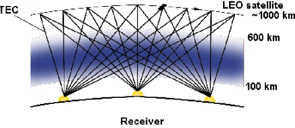
Figure 1 shows a typical LEO satellite and ground-based re-ceiver configuration used for ionospheric tomography. For clarity sake only three receivers are shown on the ground,
Fig. 1. The geometry for ionospheric tomographic imaging, showing the ray paths between a low orbiting satellite and ground receiving
stations.
which simultaneously observe the LEO satellite, at an alti-tude of ∼1000 km from the ground. The total duration of the satellite passes is typically ∼10–20 minutes. In the present study, five receiver locations are considered at 8◦N, 13◦N, 17◦N, 23◦N and 28◦N latitudes. These approximately cor-respond to the latitudes of the Indian tomography network stations. For the forward modelling, the ionospheric den-sity is assumed to be piecewise constant. For our simula-tions, geocentric circular grids, having a resolution of 2◦(in
latitude)×50 km (in altitude), are used.
Each line connecting the satellite position and the ground receiver represents one TEC measurement along the line of sight. When all three receivers simultaneously observe the satellite, as represented by lines connecting satellite and re-ceivers, the region having the maximum number of ray path intersections signifies maximum TEC information along dif-ferent directions. The TEC information content decreases as the number of intersecting ray paths decrease in the latitude-altitude space. In the present study, this space spans from 7◦N to 29◦N in latitude and 100 to 550 km in altitude. The modelling grid is superimposed on the measurement space defined by the satellite and receiver configuration. As men-tioned earlier, electron densities are assumed to be constant within each grid. The slant TEC is the sum of the small ray elements within a grid multiplied by the electron densities in the corresponding grid, along each line of sight. Using this information, the electron density distribution in the region is reconstructed.
In our forward model estimations, the IRI model is used to generate the background ionospheric densities over which various structures are artificially introduced. These struc-tures include electron density enhancements and depletions with various latitudinal extents. In fact, these structures are often present in the ionosphere over equatorial and low lat-itudes. Three distinct ionospheric conditions are considered for inversion in the present study. As mentioned earlier, the forward model to compute the data (TEC’s) basically uses
the piecewise constant discretization approach. The TEC samples were calculated for every 3-sec interval, to obtain a proper sampling, and also to ensure enough intersecting ray paths through grids. This is quite a realistic sampling, be-cause for the Indian tomography experiment all the receivers have a scan rate of 100 samples per second. This means that a proper time averaging can be performed, which can obvi-ously increase the quality of the data. The same resolution of 2◦×50 km is preserved for reconstruction also. As a first
sim-ulation step, the input TECs are assumed to be representing the absolute TECs along the slant path, connecting the satel-lite position and the receiver without any measurement error. The SVD algorithm is used for all reconstructions, which do not require any start profile. This ensures the elimination of the possibility of errors due to improper initial profiles.
5 Results and discussion
5.1 Case 1: a geomagnetically quiet ionosphere
The background ionospheric density for each grid point be-tween 7◦N to 29◦N latitude and 100 to 550 km in altitude, for a geomagnetically quiet ionosphere, are derived using the IRI model. The IRI model is run for 12:00 local time, as-suming a sunspot number of 100. Though the IRI for these conditions predicts a minor increase in the electron density around 17–22◦N latitude, the latitudinal variation of
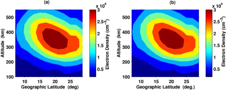
elec-tron density predicted by the IRI model is too small to rep-resent the EIA associated density enhancements. Therefore, this prediction (Fig. 2a) represents a geomagnetically quiet, low-latitude ionosphere without any major structures present therein.
Figure 2b shows its reconstruction using the SVD algo-rithm. It is seen that there is a fairly good match among these two in retaining the latitudinal as well as altitudinal extents of the electron density distribution in the reconstruc-tion. The maximum difference from the input distribution,
Fig. 2. (a) The model ionosphere used for generating TECs. (b) The tomographic reconstruction corresponding to Fig. 2a.
Fig. 4. Three typical vertical profiles. The continuous curve represents the model electron density profiles and the points are the result of the
tomographic inversion.
Fig. 5. (a) Same as Fig. 2a but with an enhanced electron density. (b) Same as Fig. 2b but with an enhanced electron density.
i.e. Fig. 2a, is less than 1%. Such a small deviation in the re-construction in this case is due to the fact that the input data is completely error free. Further, the assumption that all the ground-based receivers are receiving satellite signals simul-taneously ensures that the geometry has a maximum number of ray path intersections.
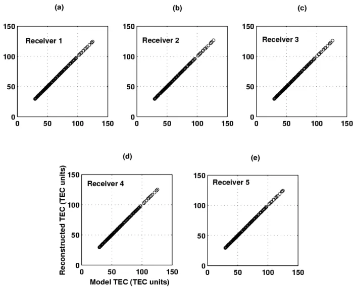
However, for checking the accuracy of reconstructions, we use two criteria. First, the reconstructed ionosphere is checked for consistency with the input ionosphere data. For this, TECs are again back calculated from the reconstructed image. Figure 3a−e shows the plots of input TECs vs. structed TECs for all five receivers. It is clear that the recon-structed TECs agree well with the input TECs. This proves that the solution obtained using SVD is consistent with the forward model. As a second criteria, the reconstructed
ver-tical ionospheric density profiles are compared with the IRI profiles at different latitudes. Figure 4a−c shows three typi-cal input IRI predicted vertitypi-cal density profiles and their re-constructions. This comparison clearly demonstrates that the two agree well, with deviations being less than 1% at the alti-tudes of peak electron density. This could be obtained when the satellite-receiver chain geometry is chosen to have a suf-ficiently large number of intersecting ray paths.
The effects of errors in the forward model estimated TECs, used for the ionospheric reconstruction on the reconstructed electron density distribution, are dealt with and discussed later.
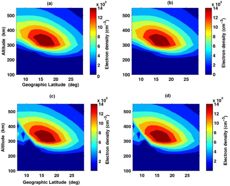
Fig. 6. (a, b) The applied model ionospheres with plasma bubbles at different altitudes. (c, d) The corresponding tomographic inversions.
5.2 Case 2: a geomagnetically quiet ionosphere with Equa-torial Ionization Anomaly
As mentioned above, the IRI does not predict the presence of EIA over the equatorial and low-latitude ionosphere real-istically. The enhancement seen in the IRI predicted density is not a true indicator of the presence of EIA. Therefore, the latitudinal distribution of ionospheric density typically asso-ciated with EIA over low latitudes is simulated and super-imposed on the IRI predicted densities for the geomagnetic conditions similar to Case 1. Thus, the obtained ionospheric density distribution that is used in the forward estimations of TECs is exhibited in Figure 5a. This figure exhibits the EIA with enhanced electron density at ∼20◦, i.e. the crest location, and trough located at ∼7◦ (geographic latitudes). These variations on electron density in the presence of EIA are quite realistic, for high solar activity periods. EIA vari-abilities of this kind have been shown to be normally present in the region of our interest, i.e. equatorial and low-latitude
region (RaghavaRao et al., 1988, and references therein). In fact, recent LITN observations show that, on a typical day, after the formation of crest at 09:00 LT, it moves poleward in the next two hours with a speed of about 1◦per hour as it intensifies. In the evening hours, it starts to weaken as it recedes equatorward with a speed of 1◦per hour (Andreeva et al., 2000).
Figure 5b shows its reconstruction which agrees well with the model input i.e. Figure 5a. The maximum deviation from the model’s vertical profile is ∼3%. In a study concerning ionospheric tomography, Andreeva et al., (2000) showed that the EIA crest concentrations can vary day-to-day by 60% in an epoch. In this context, since the vertical profile esti-mates at the crest location agree within 3% in the present study, it is possible to investigate the day-to-day variations of crest concentrations with this experimental configuration. Nonetheless, the accuracy in the crest location is determined by the horizontal grid resolution, i.e. 2◦in the present study.
Fig. 7. Distribution of singular values for the geometric matrix A.
Moreover, with the long receiver chain of Indian tomogra-phy experiments that covers the typical EIA region, it will be possible to image the movement of EIA during the course of a day.
5.3 Case 3: plasma bubbles
Equatorial bubbles (ESF) are the depletions in equatorial F region plasma that occur after sunset on the bottom side of the F layer and rise to high altitudes. Observing these bubbles is difficult, because they are unpredictable in the time and location of occurrence, and are highly variable in latitudinal and longitudinal extents, as well as in drift velocity and life time (Whalen, 1997). It is seen that the polarization electric field associated with the ESF irregularities can map for long distances along the magnetic field and can thereby influence even the lower altitude plasma (Vickrey et al., 1984).
To understand the ability to reproduce such bubbles by the present tomographic network of receivers, we have simulated plasma bubbles at different altitudes. Figures 6a and 6c show the model surfaces with depletions in electron densities. The IRI model is run for 20:00 local time, giving typical sunspot maximum conditions. This represents a typical background electron density distribution of nighttime ionosphere. For Fig. 6a, a small depletion of 30% is introduced at 250 km, at the 7◦-9◦grid, and then it is mapped to the off-equatorial latitudes following Farley’s equation that describes the map-ping of ionospheric structures along the magnetic field lines (Farley, 1960). Similarly, for Fig. 6c, a depletion of ∼90% is introduced at 400 km, at the 7◦-9◦grid, and then it is mapped to the off-equatorial latitudes.
Figures 6b, and 6d show their reconstructions, respec-tively. It is clear that the present network is able to image the ionosphere with such bubbles present at different altitudes. In the present case, with error free TEC values, the devia-tions are within 1%. However, the presence of larger errors can make the reconstruction unable to represent the smaller
depletions. The effect of errors in such situations is discussed later. Apart from equatorial bubbles, we come across plasma density depletions, during magnetic storms also, which were observed in the experiments of the LITN. It has been ob-served during a moderate magnetic strom that the steep den-sity gradients in the electron densitites, within a span of 2◦, can differ by a factor ranging from few times to about 1 order of magnitude at various regions of the equatorial ionosphere Ji-Sheng et al., 2000). Our study shows that with the present receiver configuration, it is possible to image such gradients also.
6 Error analysis
In actual experimental situations, the observed data contain different kinds of errors. For the tomography problem, the main sources of errors in TEC’s are (i) the unknown con-stants in the TEC estimates, (ii) measurement errors and (iii) discretization errors. The unknown constants in TEC arise because of two reasons, (i) the receiver biases and (ii) the incorrect estimation of the cycles in the phase measurement. The unknown constants are those that get added up as a con-stant to each measurement, either due to receiver errors or due to the unknown initial phases or 2nπ ambiguities in the differential Doppler measurements. These can be resolved to an extent by having independent ionosonde measurements at the receiver latitudes.
The ionosonde provides electron density profiles only up to the altitude of maximum electron density (bottom-side profiles). This would give vertical TEC estimates up to the altitude of maximum electron density. The topside profiles are estimated from models and used for obtaining vertical TEC estimates for the topside. A combination of these two gives the vertical TEC measurement at the receiver location. This is used for the estimation of the unknown constant in TEC in the differential Doppler measurement. Typically, the measured slant TECs are of the order of a few tens of TEC units. Considering an average value of 50 TEC units as a typical measurement, the error of 1% in TEC gets translated to an error of 8 radians. This corresponds to approximately one cycle in the phase measurement. In our simulations, the errors in the TECs range from 1–5%, corresponding to an error of a few radians in phase estimations, which are quite realistic. For example, the bias errors added are 1% and 5% of the minimum TEC (which is ∼25 TECU in the first case), so the errors correspond to 4 radians and 20 radians of phase error.
The random errors generally occur due to the sudden loss of data, by discontinuities in the differential phase measure-ments that introduce the phase measurement errors for a short duration. These can be clearly seen in the phase data itself. Such data can be rejected, or if the discontinuity is for a short duration the data can be linearly interpolated, without much effect (Leitinger, 1994). Similar to the case of bias errors, the errors added in this case also correspond to errors up to
Fig. 8. (a) The model ionosphere for error analysis. (b) The reconstructed image, with a bias error of 1% of the minimum TEC when the 3
smallest singular values are omitted from the solution. (c) The difference from the model.
a few radians in phase measurement, which is quite possible in real situations.
The next source of error comes from the discretization used for the reconstruction. This is because the actual distri-bution of electron density in the distridistri-bution is not discrete, but continuous. So, the variations in the actual ionosphere are continuous rather than discrete. All reconstruction algo-rithms will be unable to reconstruct such continuous varia-tions, so the image accuracies will be limited by the grid size chosen for reconstruction. To quantify such errors, the TECs should be calculated using integrals, which represent the ac-tual ionosphere. This error is inherently associated with the grid geometry of the reconstruction, which can be reduced by reducing the size of each pixel (Kunitake et al., 1995).
We have estimated the effect of bias errors, the random errors and the discretization errors on the accuracies of the reconstructed images separately. As mentioned earlier, the truncation of the singular values are extremely important, when the data is erroneous. Figure 7 shows the distribution of all the singular values of the geometry matrix used.
7 Bias errors and random errors
Firstly, the geomangentically quiet ionosphere without any major structures is considered for error analysis (same as Fig. 2a). Figure 8a shows this model. The TECs are esti-mated from this model and various biases are added to those values. For example, Fig. 8b shows the reconstructed image when a bias error of 1% of the minimum TEC is added to the input data. For obtaining this image, the smallest 3 singular values are omitted from the solution. If we include all the singular values, it is seen that the reconstructed image is not able to reproduce the input electron density distribution (not illustrated). Figure 8c shows the difference between input and reconstruction.
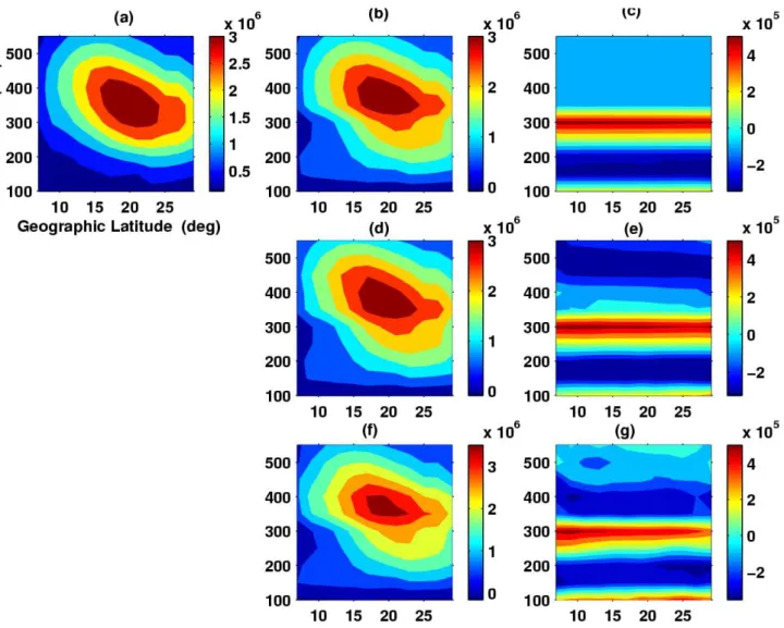
Figure 9a shows the model which is the same as the ear-lier one, but another reconstruction is performed with a bias error of 5% of the minimum TEC added to the input data. Figure 9b shows the reconstruction with the 3 smallest
val-ues truncated. We can see that the solution still deviates from the model. Figure 9d shows the image obtained when the 4 smallest singular values are truncated. This can be consid-ered as the best solution, because when more singular values are truncated the solution shows again more deviations. Fig-ures 9f and 9h represent the cases when the 5 smallest and 8 singular values are truncated. Figures 9c, e, g and i show the corresponding differences from the model for these three cases. In Fig. 9b, where some of the smaller singular val-ues with errors are also present, the reconstruction is unable to represent the layered structure. This is because of the er-ror magnification due to the presence of the smaller singular values, which tend to perturb the solutions. The presence of one more singular value makes a significant difference in the reconstruction, as most of the features are not reproduced, neither spatially, nor in magnitudes. In Fig. 9d, also, it can be seen that the peak position, as well as the magnitude of the peak electron density, has changed, where both the lati-tudinal and altilati-tudinal extents of the peak electron densities differ substantially (as high as ∼50%). So, it is quite rea-sonable to attempt another reconstruction with more singular values truncated. But the truncation of more singular values also causes significant deviation from the model. As more and more singular values are truncated, the solution tends to become smoother (Figs. 9f and 9h). This is because the sin-gular values contain the actual information about the system, and in truncating the singular values we are actually avoiding some part of the information also, so there is always an opti-mal truncation where we can reduce the error magnification to obtain the best solution, which for this particular geometry is 4.
On similar lines, the effect of random errors in the recon-struction is also estimated. The model used for generating the TEC values is shown in Fig. 10a, which is again the same as Fig. 2a, representing a geomagnetically quiet day-time ionosphere obtained using IRI-90 model without any major structures present therein. Random numbers ranging from 0.001% to 1% of the average TEC value are added to the forward model estimated TECs as errors. This corre-sponds to the situation where some of the observations are
3454 S. V. Thampi et al.: Simulation studies
34
Figure 9 a-i
Fig. 9. (a) Same as Fig. 8a. (b) Reconstruction with a bias error of 5% of the minimum TEC when the 3 smallest singular values are truncated.
(d) Reconstruction with a bias error of 5% of the minimum TEC when the 4 smallest singular values are truncated. (f) Reconstruction with
a bias error of 5% of the minimum TEC when the 5 smallest singular values are truncated. (h) Reconstruction with a bias error of 5% of the minimum TEC when the 8 smallest singular values are truncated. (c, e, g, i) The corresponding differences from the model in Fig. 9a.
more erroneous than others, which represents a real experi-mental case. Figure 10b shows the reconstruction where the lowest 3 singular values are truncated, and Fig. 10d shows the reconstruction with the lowest 4 singular values truncated. Figures 10c and 10e represent the difference plots for the two cases, respectively. Here, also, truncation plays a very
impor-tant role in the image accuracies. In this case, also, another reconstruction is done with the 5 smallest values truncated (Fig. 10f). Figure 10g shows the deviation from the model. Here also, the image becomes too smooth, and hence unac-ceptable.
Fig. 10. (a) Same as Fig. 8a. (b) The reconstruction with random errors ranging from 0.001% to1% of the average TEC added to input data
and with the 3 lowest singular values truncated. (d) The reconstruction with random errors ranging from 0.001% to1% of the average TEC added to input data and with the 4 lowest singular values truncated. (f) The reconstruction with random errors ranging from 0.001% to1% of the average TEC added to input data and with the 5 lowest singular values truncated. (c, e, g) The corresponding differences from the model in Fig. 10a.
It should be mentioned here that random errors can pose a serious problem in the accuracy of reconstruction, and such errors should be identified and tackled before using the data for reconstruction. This is necessary because in an actual case, random errors can appear with any magnitude, and the presence of such errors, if overlooked, can give wrong solu-tions. But if the random errors can be identified in the raw data itself, such errors in reconstructions can be avoided.
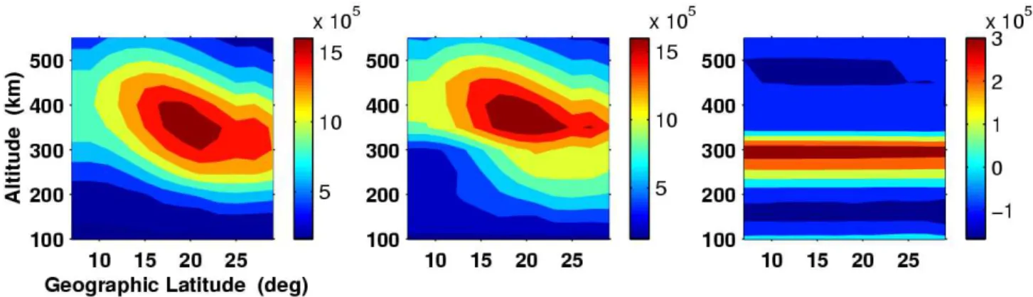
As the CRABEX aims at imaging the equatorial and low-latitude ionosphere, which is replete with processes like EIA and plasma bubble, such cases are also used for the present study. Figure 11a represents the model ionosphere, with EIA. Figure 11b is its reconstruction with 1% of the minimum TEC added to the data as bias error. Figure 11d is a similar case with 5% of the minimum TEC as bias error. Figure 11f is the reconstruction, with random errors of magnitude rang-ing from 0.001% to1% of the average TEC, added to the data.
Figures 11c, 11e and 11g are the corresponding differences from the model. Here the reconstruction is shown with op-timal truncation only, i.e. in all these cases the four smallest singular values are truncated. The effect of truncating more or less the number of singular values is very similar to that of the earlier case, i.e. model ionosphere without any ma-jor structures present therein. Another striking aspect is that the image accuracies are much higher than the previous case (maximum deviations are of the order of 15%−25%). This means that the present network is able to image the EIA and the variability associated with it quite effectively. Or, in gen-eral, we can say that large-scale structures can be imaged with reasonable accuracies using tomography techniques.
But when we have to image the ionosphere with structures having relatively smaller density gradients, the errors pose many severe problems. This can be observed in a simulation where we have tried to reconstruct a small plasma bubble
Fig. 11. (a) Model ionosphere with an enhanced electron density. (b) The reconstructed image with a bias error of 1% of the minimum TEC
when the 3 smallest singular values are omitted from the solution. (d) Reconstruction with a bias error of 5% of the minimum TEC when the 4 smallest singular values are truncated. (f) The reconstruction with random errors ranging from 0.001% to1% of the average TEC added to input data and with the 5 lowest singular values truncated. (c, e, g) The corresponding differences from the model in Fig. 11a.
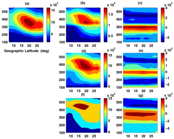
(∼30% depletion), with errors added to the data. Figure 12a shows the model, and 12b is its reconstruction, with 1% of the minimum TEC added to the data as bias error. Figure 12d is another case with 5% of the minimum TEC as bias error. Figure 12f is the reconstruction, with random errors added, the maximum being 1% of the average TEC value. Figures 12c, e, g are the corresponding differences from the model. It can be seen that, even though the depletion in the model is present in the reconstruction, there are additional artifacts in the image. Also, some of the deviations are of the order of the depletion itself, or more, which makes the image reliability substantially low. So, we can say that, if errors are present in the data, the accurate imaging small electron density gradients will be extremely difficult, but large-scale structures and gradients can be quite accurately imaged.
8 Discretization errors
So far we have discussed the errors associated with the data. The other important error which limits the accuracy of the to-mographic images is the discretization error, which is inher-ent in the system. As minher-entioned earlier, the variability in the ionosphere is continuous rather than discrete, and the mea-sured TECs are integrals, so any kind of discretization will have a certain amount of error associated with it. To under-stand the effect of discretization, we have performed some simulations, first with the ionosphere without much struc-tures, and then with an ionosphere having EIA.
Figure 13a shows the model. For generating the input, each ray path between 100 and 550 km was divided into 450 (step of 1 km) and the TECs are generated as integrals. Re-construction is performed again, as in the previous cases, for a 50-km vertical grid resolution, and the image obtained is shown in Fig. 13b. We have omitted the three smallest
sin-Fig. 12. (a) Model ionosphere with an electron density depletion of 30%. (b) The reconstructed image, with a bias error of 1% of the
minimum TEC when the 3 smallest singular values are omitted from the solution. (d) Reconstruction with a bias error of 5% of the minimum TEC when the 4 smallest singular values are truncated. (f) The reconstruction with random errors ranging from 0.001% to1% of the average TEC added to input data and with the 4 lowest singular values truncated. (c, e, g) The corresponding differences from the model in Fig. 12a.
gular values in this case, which are seen to be the optimal truncation. If we include more singular values, the solution has larger perturbations, and the solution with a lesser num-ber of singular values tends to be smoother (not illustrated). In a similar manner, we have considered the case of EIA also. Figure 14a shows the model and 14b shows the image with optimal truncation, in which we have omitted the three small-est values. It can be seen that for both these cases, the error due to discretization is significant. As discussed in Kunitake et al. (1995), we can attribute this as being due to the approx-imation in TEC to a finite dimensional expression Y =Ax. To reduce the discretization error, the size of each pixel should be reduced. This will make the number of pixels much larger; hence, the matrix size will be much larger.
All these errors, when present, generally make the recon-struction inaccurate. However, in actual cases, more than one inversion procedure can be followed and the image
ac-curacies can be enhanced by averaging all of the images in the assembly of solutions (Andreeva et al., 2001).
9 Conclusion
The present simulation study shows that the SVD technique can be used with certain limitations for tomographic studies. This technique is useful to understand the effect of receiver configuration on the reconstructed ionospheric images. In SVD, the singular values contain the information about the system, and when errors are associated with the data, the presence of smaller singular values amplify the numerical error during inversion, thus causing perturbations in the so-lution. So, we have to truncate the singular values to ob-tain the best solution. Including more singular values will cause larger perturbations, while avoiding more singular val-ues tends to yield an over-smooth solution. So there is an
Fig. 13. (a) The model used to study the discretization error. (b) The tomographic reconstruction corresponding to Fig. 13a.
Fig. 14. (a) The model with an enhancement in electron density, used to study the discretization error. (b) The tomographic reconstruction
corresponding to Fig. 14a.
optimum value for truncation, which, in the present case, is seen to be the truncation of the 4 smallest singular values for the case of data with errors. The effect of the discretization error is also studied, for which the truncation of the 3 sin-gular values gave the best solution. These simulations are extremely important in view of the experiment, because the data will always contain errors.
As mentioned earlier, in the Indian tomographic network of receivers, the measured data is the differential Doppler, which is proportional to the slant relative TEC. Since we are measuring the relative phase only, the measured phase has an arbitrary starting point. So, we have to add an ini-tial phase to obtain the true relative phase. In practice, this is achieved through independent measurements. However, any inaccurate estimation of the initial phase is a significant
source of error. These are the sources of unknown constants or bias errors in the data. The errors due to an unknown ini-tial phase can be minimized effectively using the phase dif-ference methods (Andreeva et al., 1992). In addition to this, there are inherent inaccuracies in measurements because of phase errors in the phase lock loops of the receiver, and the overall phase change due to antenna pattern and noise. These are probably of a magnitude of 2π /10 at the 50 MHz level (Leitinger, 1994). This also adds to the errors in the data, most of which are really random in nature. Averaging meth-ods can minimize the random errors in the solution. Even with all these error minimization procedures, the data will still not be completely error free. So, we have estimated the effect of the errors in the accuracies of reconstruction.
The difference in the reconstruction caused by various er-rors varies from a few percent to as large as 50%. The bias errors and random errors cause deviations, both in the case of the ionosphere without any major structures, as well as for the case of EIA. The image accuracies are much higher for the case with EIA (maximum deviations are of the order of 15%−25%). Apart from data errors, the discretization used for the imaging is an inherent source of error. The effect of discretization is also understood using simulations. How-ever, the effect of this error can be minimized by reducing the pixel sizes (Kunitake et al., 1995).
The simulations helped to understand that by using the co-herent radio beacon (CRABEX) network of the Indian to-mography experiment, it would be possible to obtain accu-rate images of the large-scale structures like EIA, which are present in the equatorial and low-latitude ionosphere. This unique chain will be able to provide valuable information re-garding the crest-to-trough ratio during varying geophysical conditions and the day-to-day variabilities and movement of the anomaly crest. The present network would also be able to image structures like equatorial bubbles, which are often present in the region, provided the processed data (after all error minimization procedures, like unknown constant esti-mations and averaging) are error free to less than 5% of the average TEC measurement.
The deviation of the reconstructed image from the model surface is only within 1% when the data do not contain any kind of errors, and the geometry is the optimum one with maximum number of path- pixel intersections. This means that solutions obtained using SVD are consistent with the data.
The present analysis highlights that tomographic imaging has the potential for evolving as a powerful tool for the inves-tigation of equatorial ionospheric structures and associated dynamics.
Acknowledgements. One of the authors, Smitha V Thampi,
grate-fully acknowledges the financial support provided by the Indian Space Research Organization through the research fellowship. Topical Editor M. Lester thanks R. Leitinger and M. Kunitake for their help in evaluating this paper.
References
Andreeva, E. S., Franke, S. J., Yeh, K. C., Kunitsyn, V. E., and Nesterov, I. A.: On generation of an assembly of images in iono-spheric tomography, Radio Sci., 36, 299–309, 2001.
Andreeva, E. S., Franke, S. J., Yeh, K. C., and Kunitsyn, V. E.: Some features of the equatorial anomaly revealed by ionospheric tomography, Geophy. Res. Lett., 27, 2465–2468, 2000.
Andreeva, E. S., Kunitsyn, V. E., and Tereshchenko, E. D.: Phase difference tomography of the ionosphere. Ann. Geophysicae, 10, 849–855, 1992.
Andreeva, E. S., Galinov, A. V., Kunitsyn, V. E., Mel’nichenko, Y. A., Tereshchenkov,E. D., Filimonov, M. A., and Chernyakov, S. M.: Radiotomographic reconstruction of ionization dip in the plasma near the Earth, JETP Lett., 52, 145–148, 1990.
Austen, J. R, Franke, S. J., and Liu, C. H.: Ionospheric imaging using computerized Tomography, Radio Sci., 23, 299–307, 1988. Bracewell R. N.: Strip integration in radio astronomy, Aus. J. Phys.,
9, 198–217, 1956.
Censor, Y.: Finite Series-Expansion Reconstruction methods. Proc. IEEE., 71, 409–419, 1983.
Farley, D. T., Jr.: A theory of electrostatic fields in the ionosphere at nonpolar geomagnetic latitudes, J. Geophys. Res., 65, 869, 1960. Foster, J. C., Klobuchar, J. A., Kunitsyn, V. E., Tereshchenkov, E. D., Andreeva,E. S., Bounsanto, M. J., Fougere, P., Holt, J. M., Khudukon, B. Z., Pakula, W., and Raymund, T. D.: Russian American tomography experiment, Int. J. Imaging Syst. Techn., 5, 148, 159, 1994.
Fougere, P. F.: Ionospheric radio tomography using maximum en-tropy, 1. Theory and simulation studies, Radio Sci., 30, 429–444, 1995.
Fremouw, E. J, Secan, J., and Howe, B. M.: Application of stochas-tic inverse theory to ionospheric tomography, Radio Sci., 27, 721, 1992.
Fremouw, E. J, Secan, J., Bussey, R. M., and Howe, B. M.: A status report on applying discrete inverse theory to ionospheric tomog-raphy, Int. J. Imaging Syst. Techno., 5, 97, 1994.
Hajj, G. A., Ibanez-Meier R., Kursinski, E. R., and Romans, L. J.: Imaging the ionosphere with the Global Positioning system,Int. J. Imaging Syst. Techno., 5, 174, 1994.
Ji- Sheng, Xu., Shu- Ying, M. A., Xiong-Bin, W. U, Lin, K. H., and Yeh ,K. C.: Tomographic imaging of low latitude ionosphere response to a magnetic storm, Chinese J. Geophys., 43, 159–166, 2000.
Kersley, L., Pryse, S. E., Walker, I. K., Heaton, J. A. T., Mitchell, C. N., Williams, M. J., and Wilson, C. A.: Imaging of electron den-sity troughs by tomographic techniques, Radio Sci., 32, 1607– 1621, 1997.
Kunitake, M., Ohtaka, K., Maruyama, T., Tokumaru, M., Morioka, A., and Watanbe, S.: Tomographic imaging of the ionosphere over Japan by the modified truncated SVD method, Ann. Geo-physicae, 13, 1303–1310, 1995.
Kunitsyn, V. E. and Tereshchenko, E. D.: Radio tomography of the ionosphere, Antenn. Prop. Mag., 34, 22–32, 1994.
Leitinger, R.: Data from orbiting navigation satellites for tomo-graphic reconstruction, J. Imag. Syst. And Technol., 5, 86–96, 1994.
Na. H, Hall, B., and Sutton, E.: Ground station spacing effects in ionospheric tomography. Ann. Geophysicae, 13, 1288–1296, 1995.
Na, H. and Sutton, E.: Resolution analysis of ionospheric tomogra-phy systems, Int. J. Imaging Syst. Techno., 5, 169, 1994. Pakula, W. A., Fougere, P. F., Klobuchar, J. A., Kuenzler, H. J.,
Buonsanto, M. J., Roth, J. M., Foster, J. C., and Sheehan, R. E.: Tomographic reconstruction of the ionosphere over North Amer-ica with comparisons to ground based radar, Radio Sci., 30, 89– 103, 1995.
Press, W. H., Flannery, B. P., Teukolsky, S. A., and Vetterling, W. T., Numerical Recipes (FORTRAN), Cambridge Univ. Press, New York, 1989.
Pryse, S. E., and L. Kersley, A preliminary experimental technique for ionospheric tomography, J. Atmos. Terr. Phys. 54, 1007– 1012, 1992.
Raghava Rao, R., Sridharan, R., Sastri, J. H., Agashe, V. V., Rao, B. C. N., Rao, P. B., and Somayajulu, V. V.: The equatorial iono-sphere, in World ionosphere- theremosphere study, WITS Hand-book, edited by C. H. Liu and B. Edwards, 1988.
Raymund, T. D., Pryse, S. E., Heaton, J. A. T., and Kersley, L.: Tomographic reconstruction of ionospheric electron density with European incoherent scatter radar verification, Radio Sci., 28, 811–817, 1993.
Raymund T. D, Austen, J. R., Franke, S. J., Liu, C. H., Klobuchar, J. A., and Stalker, J.: Application of computerized tomography to the investigation of ionospheric structures, Radio Sci., 25, 771– 789, 1990.
Vickrey, J. F., Kelley, M. C., Pfaff, R., and Goldman, S. R.: Low-latitude image striations associated with bottomside equatorial spread F: observations and theory, J. Geophys. Res., 89, 2955, 1984.
Whalen, J. A.: The equatorial anomaly: Its quantitative relation to equatorial bubbles, bottomside spread F and ExB drift veloc-ity during a month at solar maximum, J. Geophys. Res., 106, 29 125–29 132, 2001.
Whalen, J. A.: Equatorial bubbles observed at the north and south anomaly crests: Dependence on season, local time and dip lati-tude, Radio Sci., 32, 4, 1559–1566, 1997.
Yeh, H. C., Franke, S. J., Yeh, K. C., Liu, C. H., Raymund, T. D., Chen, H. H., Izotov, A. V., Liu, J. Y., Wu, J., Lin, K. H. and Chen, S. W.: Low- latitude ionospheric tomography network along Tai-wan meridian, in Low latitude ionospheric physics, edited by Fu-Shong Kuo, Elsevier Sci, NY, 1994.
Yeh, K. C., Franke, S. J., Andreeva, E. S., and Kunitsyn, V. E.: An investigation of motion of the equatorial anomaly crest, Geophy. Res. Lett., 28, 4517–4520, 2001.
Zhou, C., Fremouw, E. J., and Sahr, J. D: Optimal truncation cri-terion for application of singular value decomposition to iono-spheric tomography, Radio Sci., 34, 155–166, 1999.