HAL Id: hal-00317708
https://hal.archives-ouvertes.fr/hal-00317708
Submitted on 3 Nov 2004
HAL is a multi-disciplinary open access
archive for the deposit and dissemination of
sci-entific research documents, whether they are
pub-lished or not. The documents may come from
teaching and research institutions in France or
abroad, or from public or private research centers.
L’archive ouverte pluridisciplinaire HAL, est
destinée au dépôt et à la diffusion de documents
scientifiques de niveau recherche, publiés ou non,
émanant des établissements d’enseignement et de
recherche français ou étrangers, des laboratoires
publics ou privés.
modelling of precipitating fluxes
C. J. Rodger, D. Nunn, M. A. Clilverd
To cite this version:
C. J. Rodger, D. Nunn, M. A. Clilverd. Investigating radiation belt losses though numerical modelling
of precipitating fluxes. Annales Geophysicae, European Geosciences Union, 2004, 22 (10),
pp.3657-3667. �hal-00317708�
SRef-ID: 1432-0576/ag/2004-22-3657 © European Geosciences Union 2004
Annales
Geophysicae
Investigating radiation belt losses though numerical modelling of
precipitating fluxes
C. J. Rodger1, D. Nunn2, and M. A. Clilverd3
1Department of Physics, University of Otago, Dunedin, New Zealand
2The School of Electronics and Computer Science, Southampton University, Southampton, UK 3Physical Sciences Division, British Antarctic Survey, Cambridge, UK
Received: 2 March 2004 – Revised: 25 June 2004 – Accepted: 17 August 2004 – Published: 3 November 2004
Abstract. It has been suggested that whistler-induced
elec-tron precipitation (WEP) may be the most significant inner radiation belt loss process for some electron energy ranges. One area of uncertainty lies in identifying a typical estimate of the precipitating fluxes from the examples given in the lit-erature to date. Here we aim to solve this difficulty through modelling satellite and ground-based observations of onset and decay of the precipitation and its effects in the iono-sphere by examining WEP-produced Trimpi perturbations in subionospheric VLF transmissions. In this study we find that typical Trimpi are well described by the effects of WEP spec-tra derived from the AE-5 inner radiation belt model for typ-ical precipitating energy fluxes. This confirms the validity of the radiation belt lifetimes determined in previous studies us-ing these flux parameters. We find that the large variation in observed Trimpi perturbation size occurring over time scales of minutes to hours is primarily due to differing precipitation flux levels rather than changing WEP spectra. Finally, we show that high-time resolution measurements during the on-set of Trimpi perturbations should provide a useful signature for discriminating WEP Trimpi from non-WEP Trimpi, due to the pulsed nature of the WEP arrival.
Key words. Ionosphere (ionization mechanisms) –
Mag-netospheric physics (energetic particles, precipitating; magnetosphere-ionosphere interactions)
1 Introduction
It has been suggested that whistler-induced electron pre-cipitation (WEP) may be the most significant inner radia-tion belt loss process for some electron energy ranges (e.g. Dungey, 1963; Rodger et al., 2003). One area of uncer-tainty lies in providing a typical description of the precipi-tating fluxes. Here we aim to solve this difficulty through modelling satellite and ground-based observations of onset
Correspondence to: C. J. Rodger
(crodger@physics.otago.ac.nz)
and decay of the precipitation and its effects in the lower ionosphere. Whistler-induced electron precipitation from the Van Allen radiation belts occurs as a result of coupling be-tween the troposphere and the magnetosphere. The ener-getic electron precipitation arises from lightning produced whistlers (Storey, 1953) interacting with cyclotron resonant radiation belt electrons near the equatorial zone (Tsurutani and Lakhina, 1997). Pitch angle scattering of energetic radi-ation belt electrons (Kennel and Petschek, 1966) by whistler mode waves drives some resonant electrons into the bounce loss cone, resulting in their precipitation into the atmosphere (Rycroft, 1973). An important parameter for determining the overall importance of WEP to radiation belt losses is the magnitude of a “typical” WEP event. This may be calcu-lated from theoretical studies (e.g. Abel and Thorne, 1998) or inferred from experimental observations, such as in-situ measurements of WEP events (Voss et al., 1998). Estimates of electron lifetimes due to WEP-driven losses using ground-based whistler observations as a proxy for WEP events took a typical WEP event as removing 0.0004% of the trapped flux (Burgess and Inan, 1993), and found that these losses might be comparable with those from plasmaspheric hiss. However, a similar study estimated that typical WEP events might remove only 0.00001% of the trapped flux (Smith et al., 2001), and hence that whistlers were not significant in overall inner-belt losses. A different approach has been to use experimental observations to characterize typical WEP magnitudes. Combining reports of satellite WEP observa-tions with ground-based whistler measurements, Rodger et al. (2003) concluded that the typical WEP mean precipita-tion energy flux was 2×10⁻³ergs cm−2s−1, and that in some
electron energy ranges WEP may be the most significant in-ner radiation belt loss mechanism.
One complementary technique to study WEP makes use of long-range remote sensing of very low frequency (VLF) waves propagating inside the waveguide bounded by the lower ionosphere and the Earth’s surface. Significant vari-ations in the received amplitude and/or phase of fixed fre-quency VLF transmissions arise from localized changes in
the lower ionosphere. Further discussion on the use of subionospheric VLF propagation as a remote sensing probe can be found in recent review articles (e.g. Barr et al., 2000; Rodger, 2003) and studies (Cummer and Inan, 2000; McRae and Thomson, 2000; Bainbridge and Inan, 2003). WEP leads to localized ionospheric modifications produced by secondary ionisation just below the D-region of the iono-sphere, which are observed as “Trimpi” perturbations in subionospheric VLF transmissions (Helliwell et al., 1973). These perturbations begin with a relatively fast (∼1 s) change in the received amplitude and/or phase, followed by a slower relaxation (<100 s) back to the unperturbed signal level due to the recombination of the additional ionisation. Trimpi perturbations permit observers to study WEP fluxes and the chemistry of the nighttime lower ionosphere (e.g. Pasko and Inan, 1994), from locations remote from the actual precipita-tion region.
Until recently, there was considerable uncertainty as to the typical size of the D-region patch altered by WEP. Trimpi perturbations have been used to show that WEP pro-duced patches are large (at least 600 km×1500 km) (Clil-verd et al., 2002), considerably larger than the observed di-mensions of whistler ducts (e.g. Angerami, 1970). Large D-region patch dimensions have been explained through a quasi-trapped whistler propagation theory in which ducted energy spreads at the magnetic equator (Strangeways, 1999), resulting in whistler-mode signals which have leaked out-side their whistler duct still contributing to the horizontal lat-eral extent of WEP. Such leakage would give a significantly larger precipitation footprint than the actual dimensions of the whistler duct. A different mechanism also leading to large WEP patch dimensions comes through the precipita-tion caused by obliquely (nonducted) propagating whistlers, creating an ionospheric disturbance of ∼1000 km spatial ex-tent (Johnson et al., 1999). At this stage there is no clear experimental evidence to indicate whether quasi-ducted or nonducted whistler propagation dominates the overall WEP losses (Rodger et al., 2003).
The decay time scale information from Trimpi signa-tures has been used to determine the vertical dimensions of the WEP modified ionospheric patches. An analysis of 134 Trimpis observed at Palmer station (Antarctica) on trans-missions from NPM (Hawaii) reported that the “recovery signatures” (decay) could be approximated by an exponen-tial function for the purposes of determining the decay rate (Pasko and Inan, 1994). A later report concluded that the decay of Trimpis follow a logarithmic dependence (Dowden et al., 2001), noting that the difference between exponential decay and logarithmic decay is relatively small, except near the beginning (near onset) and end of the perturbation. This study also noted that a re-examination of Trimpi observed in Tokyo from NWC (Australia), were also consistent with a logarithmic decay signature, rather than an exponential decay with two characteristic time scales, as originally concluded (Molchanov et al., 1998).
A number of theoretical studies have made use of elec-tron density perturbations with a vertical Gaussian profile
to represent the WEP produced ionospheric electron density modification (Nunn and Strangeways, 2000; Clilverd et al., 2002), while others have studied modifications derived from satellite observed WEP fluxes (e.g. Pasko and Inan, 1994; Rodger et al., 2002). For example, it has been reported that the observed Trimpi recovery signatures may be used to de-termine the energy content of WEP bursts (Pasko and Inan, 1994). In this paper we closely examine the onset and decay of Trimpi perturbations so as to better understand the WEP fluxes producing the ionospheric modification, characterized through experimental WEP observations, and thus investi-gate the estimates of the likely impact of the WEP on the radiation belts.
2 Modeling Trimpis due to WEP impact
In this section we define the process through which we attempt to understand the nature of precipitation fluxes by modelling a specific set of precipitation conditions (transmitter-receiver great circle path) described by Clilverd et al. (2002), combing flux spectrum observations, a model of the atmosphere, and a VLF scattering model.
2.1 Scattering model and situation
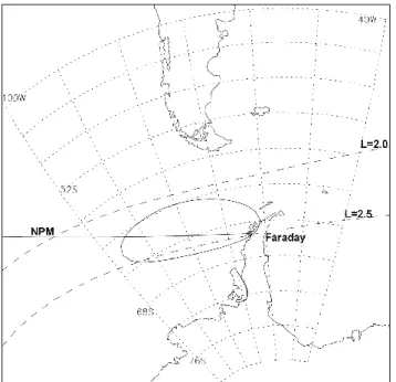
We consider the VLF Trimpi perturbations that have been observed at the Faraday research station (65.3◦S,
64.3◦W, L=2.5), Antarctica, on transmissions from NPM
(23.4 kHz, Oahu, Hawaii). The WEP is taken to produce an ellipse-shaped ionospheric modification with dimensions 850×2150 km, centred 800 km away from Faraday on the 12.3 Mm NPM-Faraday great circle path (GCP), the ellipse having its long axis orientated in the magnetic E/W direction as shown in Fig. 1. The WEP-modified ionospheric modi-fication is termed a Lightning Induced Enhancement (LIE) “patch”. This position and ionospheric modification size are taken from Clilverd et al. (2002), and are determined by ob-servations at multiple Antarctic Peninsula stations. Inside the WEP modified ionospheric region the perturbation to the collision frequency profile is assumed to be zero due to rapid plasma cooling (∼0.1 s at 85 km, and faster for lower alti-tudes; Rodger et al., 1998), and thus the modification is de-scribed solely in terms of perturbations to the electron num-ber density profile dNe(x,y,z), determined in Sect. 2.2 and
taken to be independent of horizontal coordinates x and y inside the LIE ellipse.
The transmitter is modelled as a vertical electric dipole at zero altitude. The receiver at Faraday is assumed to be a ver-tical electric dipole antenna, though in experimental practice the horizontal magnetic fields are measured with a loop an-tenna. Apart from the WEP modified ionospheric patch the background ionosphere is assumed to be homogeneous along the GCP. The unperturbed ionospheric electron density and collision frequency profiles are given by a standard nighttime
Fig. 1. Map of the region around the Antarctic Peninsula, showing
the location of Faraday Station. The Great Circle Path to the trans-mitter NPM is plotted, along with the L=2.0 and L=2.5 contours at 100 km altitude. An ellipse marks the WEP modified ionospheric region used in our calculations.
ionospheric model. The effective collision frequency (υ) profile is given as a function of vertical coordinate z, by
υ(z) =1.816 × 10¹¹e−0.15z [s−1], (1) while the unperturbed electron number density profile,
Ne(z), at D-region altitudes is specified by a Wait ionosphere
(Wait and Spies, 1964),
Ne(z) =7.855 × 10⁻⁵eβ(z−h
0
)υ(z) [el. cm−3]. (2)
Here β represents the “sharpness” of the lower ionospheric boundary and h0 represents the effective height of the
iono-sphere, taken as being h0=87 km and β=0.5 km−1 (dashed line) for typical nighttime conditions. The neutral atmo-sphere is described using the MSIS E-90 model atmoatmo-sphere (Hedin, 1991) for (62.5◦S, 280◦E, L=2.23), roughly the cen-tre of the patch, for 06:00 UT, 23 April 1994. The ground’s electrical properties also are assumed to be homogeneous and to have the properties of seawater, with conductivity 4 S m−1, and dielectric constant of 81.
2.2 Production of ionospheric modification from WEP The differential number spectrum as a function of energy of our “typical” WEP burst, N (E), is found as described in Rodger et al. (2003), assuming an electron beam limited to the range 1–1500 keV, produced by a whistler spanning 0.5– 5 kHz with power spectral density as given by the lightning spectra. It is assumed that the WEP lasts 0.2 s, and has a mean precipitation energy flux of 2×10⁻³ergs cm−2s−1. A cold plasma density from Menk et al. (1999) is taken. In our
Fig. 2. Differential electron number flux of precipitated electrons in
WEP events versus energy, showing the two different energy spectra used to characterize the bursts. The heavy line uses the empirical AE-5 trapped electron model, while the lighter grey line uses an
e-folding energy of 120 keV.
initial calculations we will consider WEP bursts with two dif-ferent energy spectra, as shown in Fig. 2. In the first case A the WEP energy spectrum is determined from the spectrum of the trapped electrons in the pitch angle range from the loss cone angle (αLC)to (αLC+ 0.5◦)given by the empirical
AE-5 Inner Zone Electron Model (Teague and Vette, 1972), after Rodger et al. (2003). In the second case B the WEP energy spectrum is taken to be proportional to exp(−E/E0), where E is the kinetic energy of a trapped electron and E0 is the e-folding energy, with E0=120 keV. This value is taken from
a detailed analysis of an experimentally observed WEP event (SEEP Event (D); Voss et al., 1998), which concluded that the differential energy spectrum of the trapped electrons for this event could be best described by E0=120±40 keV (Inan
et al., 1989). Note that this e-folding energy is roughly two and a half times bigger than that found for case A, leading to a WEP burst (B) having a greater high-energy contribution, as seen in Fig. 2.
The ionospheric effects due to each type of WEP burst may be determined by convolving the ionisation rate for a monoenergetic electron beam with the differential number spectra, N (E) shown in Fig. 2, and integrating over the en-ergy range 1–1500 keV. The WEP burst ionisation rate q(E) is found by an application of the expressions in Rees (1989), as has been previously described by Rodger et al. (2002). 2.3 Relaxation of WEP-modified regions
The relaxation of the WEP-induced ionisation is calculated from the end of the WEP burst, which is taken to be at t =0, assuming no changes to the WEP ionospheric modifications during the burst, i.e. that the relaxation time is significantly longer than the 0.2-s burst. Electron loss rates are calcu-lated using reasonable values for the attachment rates and recombination coefficients at ionospheric altitudes (Rodger
Fig. 3. Relaxation of different ionisation changes in the lower
iono-sphere at various times after the creation of the WEP-produced patch. The initial change at t=0, and the ambient night-time elec-tron density profile, are shown as heavy lines. (a) Ionisation pro-duced by the AE-5 WEP burst to the lower ionosphere. (b) Ionisa-tion due to the e-folding profile.
et al., 1998), previously used to investigate red sprite associ-ated ionisation (Nunn and Rodger, 1999) and solar eclipses (Clilverd et al., 2001). Ambient electron production rates (separate from WEP) are calculated by assuming that the ionosphere is initially in equilibrium. As such, the simulated ionospheric electron density will relax towards the ambient profile from any perturbed state. The loss rates given by the Rodger et al. (1998) expressions depend on the temperature of the electrons and neutrals present and on the instantaneous electron density. While WEP events are likely to cause sig-nificant changes in electron temperature, these will be short-lived in comparison with modifications to the electron den-sity (Rodger et al., 1998). Thus, throughout our simulation, the electron temperature is taken to be equal to the neutral temperature.
The relaxation of the ionisation changes for the WEP-pulses (Fig. 2) are shown in Fig. 3. In both panels of this figure the heavy line shows the total electron density caused by the 0.2-s WEP burst at t =0, before the ionisation starts
to relax towards the ambient profile (also shown as a heavy line). A number of intermediate ionisation profiles are also shown on the figure describing the ionisation profiles for various times after the WEP disturbed patch is created. In reality, the ionisation profiles Ne(z)+dNe(z,t ) have been
de-termined with higher time resolution than shown in this fig-ure; in the first 30 s the maximum time resolution of the ioni-sation profiles is 0.4 s, followed by longer, nonlinear steps at the tail-end of the perturbation.
2.4 Scattering theory and implementation
The linear Born theory of 3-D VLF scattering from an ionospheric plasma perturbation is fully described in Nunn (1997). The Born approximation involves assuming that the total incident field at a given point in the LIE is the incident zero order field (E0). As shown by Nunn (1997), a better
linearization may be achieved by assuming that the perturba-tion of the electric displacement vector is zero within the LIE rather than that the perturbation of the electric field is zero. The modified region is covered by a 3-D spatial grid, and the zero-order incident field E0 calculated for each grid point.
VLF propagation from the transmitter to each grid point is computed using modal theory and the Naval Ocean Systems Center (NOSC; San Diego, USA) MODEFNDR code (Mor-fitt and Shellman, 1976). The MODEFNDR code returns all the parameters of the subionospheric VLF modes, as de-scribed by Wait (1996). MODEFNDR receives as inputs the frequency, as well as the ionospheric and geomagnetic pa-rameters. Then, assuming horizontal homogeneity, but tak-ing into account the curvature of the Earth, the program cal-culates the appropriate full wave reflection coefficients for the waveguide boundaries and searches for those complex modal angles which give a phase change of 2π across the guide. At each grid point, linear scattering theory furnishes an effective current Jeff(r) which acts as the source of the
scattered field Es. Clearly, for large LIE patches and/or
patches with large changes in electron number density the Born approximation will break down, since the total field at a point in the LIE will not be well approximated by the zero-order incident field. By comparing with a 2-D Finite Element modelling of VLF scattering, it was shown in Nunn et al. (1998) that for an LIE with horizontal dimensions ∼100 km the Born approximation fails for maximum electron density perturbations >6 el. cm−3.
The current version of the code neglects all components of the conductivity tensor, except the zz component. When the transmitter and receiver are both vertical electric dipoles, this is amply justified to an overall accuracy of the order of a few percent (Clilverd et al., 1999). The vertical electric field at the receiver is computed for each elementary volume of the modified region using MODEFNDR, summed over the total modification volume to give the total scattered field, and thus the observed VLF perturbation. The height gain functions re-turned by MODEFNDR become inaccurate at high altitudes, although generally for those altitudes above the VLF reflec-tion height. Accordingly, an attenuareflec-tion funcreflec-tion has been
applied to these functions to prevent an incorrect contribution appearing due to ionisation at heights >85 km. This attenua-tion funcattenua-tion is piecewise linear and was derived from a sepa-rate calculation that integsepa-rates the Booker quartic through the ionosphere for the dominant TM VLF modes. Contributions to VLF scattering from high altitudes are therefore estimates based on the attenuation function applied to the height-gain functions. We expect any inaccuracies to be small, as the presence of a significant high altitude scattering contribution would lead to a long tail in the Trimpi time signature, which is not seen in experimental observations. In future studies it is proposed to replace MODEFNDR with a full wave prop-agation code or a substantially modified version of MOD-EFNDR. This code has previously been used to study the size of WEP produced ionospheric patches (Clilverd et al., 2002), and the relaxation of ionospheric ionisation produced by red sprites (Nunn and Rodger, 1998).
2.5 LIE characteristics based on WEP bursts
Using the ionisation profiles Ne(z)+dNe(z,t ), in association
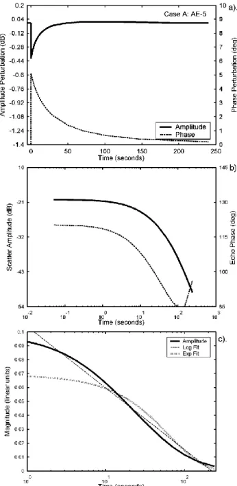
with the 3-D scattering code, we have calculated the time-varying NPM VLF perturbations expected at Faraday due to the relaxing ionospheric modifications shown in Fig. 3. The resulting perturbations from the undisturbed wave due to an AE-5 WEP burst (case A) are shown in the top panel of Fig. 4. The heavy black line shows the perturbation to the received amplitude, while the dashed line gives the pertur-bation in the received phase. As expected for perturpertur-bations due to large homogenous modifications straddling the GCP, the transmission amplitude decreases while the transmission phase increases (Wait, 1964). As the ionospheric modifica-tion relaxes, the perturbamodifica-tions decay back to the undisturbed level. Note that the phase perturbation returns to the unper-turbed level considerably more slowly than the amplitude perturbation, as observed in experimental data (e.g. Dow-den et al., 2001). This phenomenon can only be due to the phase of the scattered signal relative to the direct signal ap-proaching an angle of ∼90◦as the perturbation decays away. There is nothing in the theory suggesting 90◦as a limiting value, and this would appear to be somewhat coincidental. Although the start of the VLF perturbation is shown in the figure, the onset is not very meaningful, as the calculations have been undertaken directly after the arrival of the WEP burst. We calculate the effects of the perturbation onset in detail in Sect. 5.
In order to consider the decay of the Trimpi perturbation we do not focus upon the amplitude or the phase perturba-tion, which are often quite different, but rather the vector combination through the standard phasor diagram (e.g. Dow-den and Adams, 1988). This produces the phasor of the wave scattered off the WEP burst plasma, which, added to the un-perturbed phasor of the NPM transmission, gives the pha-sor of the perturbed wave. We call this the scatter phapha-sor, which has magnitude, M, and phase, φ, (to avoid the confus-ing nomenclature of “scatter phasor phase”, φ has often been referred to as the “echo phase”). As seen in the middle panel
Fig. 4. VLF perturbation (“Trimpi”) calculated for NPM
transmis-sions received at Faraday due to an ionospheric perturbation caused by a WEP burst with AE-5 energy spectra (case A) The top panel shows the perturbations in amplitude and phase, while the middle panel shows the calculated scatter magnitude and phase which pro-duces this Trimpi. The lower panel shows the decaying scatter mag-nitude plotted on a logarithmic timescale after Dowden et al. (2001), with logarithmic (dashed) and exponential (dash-dot) fits.
of Fig. 4 the echo phase approaches ∼90◦ as the perturba-tion decays, as noted above. The lower panel of Fig. 4 shows the decay of the scatter magnitude, M, on a logarithmic time scale. The scatter amplitude time decay features and their fit to the observations of Dowden et al. (2001) will be described in Sect. 4.1 below.
Fig. 5. VLF perturbation in the same form as that shown in Fig. 4,
but in this case caused by a WEP burst with an e-folding energy spectra (case B).
Similarly, the calculated VLF perturbations created by the
e-folding WEP burst (case B, Fig. 3b) are given in Fig. 5, in the same format as Fig. 4, for comparison with experimental observations.
3 Comparison with experimental observations
3.1 Temporal decay signature
The shapes of the decaying VLF perturbations shown in Figs. 4a and 5a resemble those observed in experimental data
(e.g. Dowden et al., 2001; Clilverd et al., 2002). For exam-ple, if one contrasts the WEP Trimpi presented in the upper panels of Figs. 10 and 11 of Dowden et al. (2001) with those in Figs. 4a and 5a one notes that the observed and calculated perturbations are positive (advancing) phase, negative (de-creasing) amplitude, that the amplitude perturbation decays to its unperturbed state faster than the phase perturbation, and that the amplitude perturbation decays to the experimental noise level (∼0.05 dB) in ∼25 s. Note that the Trimpis pre-sented in the Dowden study were chosen on the grounds they are unusually large, and therefore well suited for examining the time decay profile of the perturbations. A comparison of the magnitudes with typical experimental data is discussed in the following section.
While the general shape of the calculated Trimpi are very similar to the experimental data, they are based on two cases of WEP fluxes with very different energy spectra. Do both cases produce the logarithmic decay profile observed experi-mentally? The decay signatures of the Trimpi amplitude and phase perturbations and the scatter magnitude are shown in Figs. 4 (case A) and 5 (case B). In the lower panels of these figures we undertake a comparison of our calculated decay-ing scatter magnitude with logarithmic (dashed) and expo-nential (dotted) fits. The experimentally observed decay of the scatter magnitude is best described through a logarith-mic decay rather than an exponential (Dowden et al., 2001). This is also true for our calculated decaying scatter magni-tude. Figure 4c shows that the logarithmic fit to the AE-5 (case A) WEP produced M over t=1 s to the end of the cal-culation period (t =240 s), which is considerably better than the exponential fit. An indication of the “quality” of the fit can be found from the departure from unity of the square of the correlation coefficient, i.e. 1−r2. For the logarithmic fit r2=0.976, but is only r2=0.895 for the exponential case (i.e. ∼4 times better fit); these values are similar to the WEP Trimpi event shown in Fig. 12 of the Dowden paper.
The situation is very similar when one considers the de-caying scatter magnitude produced by the e-folding WEP burst (Fig. 5c). Again, the logarithmic fit is considerably better at describing the decay process (r2=0.972) than the exponential (r2=0.83). Clearly, there is no significant dif-ference between the quality of the logarithmic fit between the WEP bursts using the AE-5 derived and e-folding en-ergy spectra. Both lead to Trimpi which decay in a manner that is typical of experimentally observed events. As the de-cay process is primarily controlled by the atmospheric model used here we can take confidence in its confirmation of the logarithmic decay times. It has been argued that the WEP fluxes derived from the AE-5 Electron Model (case A) should be more typical than those described by an e-folding energy of E0=120 keV (case B), as the latter is based on a single
measurement (Rodger et al., 2003). We investigate this more closely in the section below.
3.2 Magnitude of perturbation
The AE-5 WEP burst (case A) shown in Fig. 4 produces a maximum Trimpi perturbation of −0.4 dB in amplitude and
+5◦ in phase (−20 dB in scatter amplitude and 120◦ echo phase). In contrast, the higher WEP fluxes at larger energies in the e-folding case (case B; Fig. 5) result in a maximum Trimpi perturbation of −1.3 dB and 8.4◦(−14 dB in scatter
amplitude and 140◦echo phase). Both are realistic in terms
of the logarithmic decay times that they produce in the at-mospheric model, as seen in the previous section. However, can we say anything about the likelihood of observing such Trimpi at any given time? Trimpi have been analyzed on the same path over an extended observation period (Clilverd et al., 1999). Trimpi with amplitude changes of >1 dB occurred on only 0.2% the of occasions, while amplitudes of >0.4 dB were nearly 50 times more common. This is also true of the relative occurrences of >8◦and >5◦phase Trimpi (0.2% of occasions and 16 times more common).
The most commonly observed Trimpi magnitude is one that is just above the noise level. This is probably because of precipitation patch location, distribution of lightning magni-tude, and changeable wave coupling into the plasmaspheric propagation path, thus altering the location and nature of the LIE. In the Clilverd et al. (1999) study there is no descrip-tion of the locadescrip-tion of the causative lightning discharge that lead to the Trimpi. Thus, our comparison with the Clilverd study above is likely to be influenced by enhanced occur-rences of smaller Trimpi caused by positional variability at the lightning source (Clilverd et al., 2002). It is also pos-sible that different lightning intensities will produce differ-ent WEP fluxes, as it is known that the WEP precipitation energy flux is proportional to the whistler wave equatorial magnetic field intensity, for most realistic wave fields (Inan et al., 1982). There are many more low current lightning events than large current ones (Uman, Fig. 7.8, 1987). This would fit the observations of many more small magnitude Trimpi perturbations than large ones. Evidence that confirms the association between lightning return current strength and Trimpi perturbation levels will be the subject of study in a fu-ture paper. As a result of these deliberations we can say that the Trimpi magnitudes given in this study suggest that the case A WEP electron spectra produce more typical Trimpi signatures than case B, given typical Trimpi observations and the typical precipitation flux employed.
3.3 Dependence upon LIE patch size
Experimental observations of Trimpi events observed on the signals from multiple Northern Hemisphere VLF transmit-ters received at multiple sites around the Antarctic Peninsula have shown that LIE patches are at least 1500 km along the major axis and perhaps 600 km along the minor axis (Clil-verd et al., 2002). Observed Trimpi show high variability in amplitude and phase from event to event. Here we test to see if varying the size of the LIE patch can significantly influence the range of Trimpi perturbations seen or if the
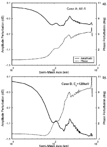
Fig. 6. Variation in the amplitude and phase of a Trimpi perturbation
caused by LIEs with varying semi-minor axis sizes (a) LIE caused by a WEP burst with AE-5 energy spectra. (case A) (b) LIE caused by an e-folding energy spectra (case B).
variability is due to other factors such as precipitation flux levels. Figure 6 shows the calculated Trimpi magnitudes for varying LIE semi-minor axis sizes. In order to maintain the elliptical nature of the LIE-patch, the major axis was var-ied in proportion to the change in the minor-axis, maintain-ing the same ellipse ratio of 2.5, and the center point at the same location 800 km west of Faraday. The variation for very large LIEs is “computational noise”, due to multimodal ef-fects, particularly due to those parts of the LIE patch very near the receiver point. This has been decreased by mak-ing calculations with a very fine grid, along with some av-eraging to decrease the significance of the noise remaining. As is clear, perturbation magnitudes increase steadily up to patch sizes of ∼200×500 km (semi-minor axis of ∼100 km), after which there is little dependence upon the size of the patch. LIE patches produced by quasi-ducted or oblique whistlers propagating in ducts would be considerably larger than 200×500 km. Combining these results with the calcu-lations presented in Clilverd et al. (Fig. 5, 2002) it appears that variations in the LIE patch size will lead to relatively small changes in Trimpi, and hence that the large variation in observed Trimpi is primarily due to changing WEP spec-tra and precipitation flux. The choice of LIE patch size will
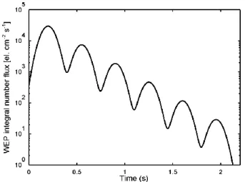
Fig. 7. Time dependence of the WEP electron flux used to simulate
the decreasing train of precipitation pulses caused by the backscat-tering of precipitating electrons.
not strongly influence the findings of our study, or alter the calculations undertaken in the Clilverd paper.
3.4 Effect of pulsed WEP on Trimpi signature
In the earlier modeling we assumed that the WEP arrived during a single 0.2-s burst. However, in-situ satellite observa-tions of WEP indicate that a portion of the precipitated elec-trons backscatter from the atmosphere and bounce repeatedly between the Northern and Southern Hemispheres, leading to a series of decreasing WEP pulses into both hemispheres over a period of ∼2–3 s (Voss et al., 1998). In order to in-vestigate this effect, we have constructed a WEP burst made up of a train of pulses, roughly modeled on the time signa-ture of the S81-1 satellite observations (Voss et al., Fig. 15, 1998). We estimate that each flux pulse was roughly half the magnitude of that occurring in the conjugate hemisphere, and therefore find the magnitude of the WEP pulse train (Fig. 7) by assuming that the ionospheric modification produced by the first pulse in the train will be half of that determined for the 0.2 s AE-5 WEP pulse (case A) in Sect. 2.2.
The time varying electron density modification has been calculated, as discussed in Sect. 2.3, using the time varying WEP pulse train. In this case, however, we allow for iono-spheric relaxation to take place during the arrival of the ∼2-s pulse train, and determine dNe(z,t) with 0.05 s time
reso-lution. The time-varying VLF perturbation calculated due to scattering from this ionospheric modification is shown in Fig. 8. Only the first 3 s of the perturbation are presented, as the pulsed nature of the WEP affects only the onset of the perturbation. Note that while additional WEP pulses arrive over ∼2 s (Fig. 7), the VLF perturbation stops responding to production of extra ionisation after ∼1.2 s into the onset phase. The ionospheric relaxation taking place between the bursts leads to a Trimpi perturbation that is slightly weaker in both phase and amplitude, such that the case A WEP spectra are even more likely to be typical.
Fig. 8. Calculated onset of VLF perturbation due to the WEP pulse
train shown in Fig. 7.
Experimental evidence for multi-burst WEP events has not been reported to date, although this may be because Trimpi observations with high enough time resolution measurements are rarely made. Nonetheless, the backscattering and bounc-ing of precipitatbounc-ing electrons is probably happenbounc-ing in the majority of WEP events, leaving an ionospheric signature which might be detectable in Trimpi perturbations. As there are a number of ionospheric processes which can lead to VLF perturbations (e.g. Rodger, 2003) similar to these “classic” Trimpi, this bursty onset might be a useful signature for dis-criminating WEP Trimpi from non-WEP Trimpi. The latter perturbations appear to be caused by much faster processes occurring inside and above thunderstorms, e.g. red sprites, elves, and sprite haloes (Rodger, 1999; Moore et al., 2003).
It should be noted that while each WEP event is made up of bursts, multi-hop whistlers are expected to precipitate sig-nificantly more electrons from the radiation belts than single hop whistlers.
3.5 Simulation of double Trimpi events
In order to test our modeling process we simulate the dou-ble Trimpi event shown in the top panel of Fig. 9. This was observed on the NPM signal at Faraday on 23 April 1994, shortly after 06:00 UT, and was selected as it is clearly de-fined and shows two events well above the noise. As seen in the figure, the initial NPM Trimpi occurs at 06:00:11 UT as a perturbation of −1.45 dB/+9.75◦, followed at 06:00:17 UT
by a Trimpi of −1.2 dB/+11.5◦, i.e. the peak of the second amplitude perturbation is slightly less than the first Trimpi, while the peak in the phase perturbation is slightly larger than the first. The first of these Trimpi is probably associated with a cloud to ground lightning discharge detected by the Na-tional Lightning Detection Network (Cummins et al., 1998), occurring at about 06:00:10 UT (33.932◦N, −74.986◦E, peak return stroke current of 136.0 kA), and located near the region known to be associated with Trimpi observed in
the Antarctic Peninsula (Clilverd et al., 2002). There are three candidate NLDN strikes at about 06:00:16 UT which could have produced the second Trimpi. All are nearby to one another and have fairly large peak return stroke currents (31.155◦N, −77.096◦E, 44.5 kA), (31.177◦N, −77.537◦E, 88.7 kA) and (31.483◦N, −77.504◦E, 61.3 kA).
We simulate this situation by using WEP spectra to create a modified ionosphere as described above, centered 800 km west of Faraday station. The ionosphere is allowed to relax for 5 s as before, after which another WEP event causes ad-ditional ionisation to be added to that which existed from the first WEP. On the basis of the modified ionosphere the time varying Trimpi has been calculated and is shown in Fig. 9 for contrast with the experimental data.
As the first of these Trimpi are comparatively large when contrasted with typical events (Sect. 4.2), we employ the case B WEP spectra to model the first burst, using a mean precipitation energy flux of 2×10⁻³ergs cm−2s−1, as
be-fore. The calculated VLF perturbation for this initial burst is shown in Fig. 9b. As the second Trimpi has a smaller am-plitude perturbation than the first, one possibility is to use a smaller mean precipitation energy flux. We find that a WEP burst using the case B WEP spectra but a flux 65% lower than the first leads to a reasonable second Trimpi, as shown in Fig. 9b. The lower mean precipitation energy flux needed to simulate the second WEP burst is probably due to combi-nation of the lower peak return stroke currents for the light-ning which may be associated with this Trimpi (∼30−65% lower), but also to less efficient coupling of the lightning en-ergy through the ionosphere to produce the WEP itself. For example, it is likely that the second set of lightning is dis-placed further from the whistler duct entry point than the first stroke, and thus might be expected to have a proportionally smaller effect. The main features of the Trimpi decay are well reproduced in the calculated events, and the perturba-tions sizes are fairly similar. The primary difference is the decay time, where both the amplitude and phase perturba-tions decay away slightly faster in the experimental data than in the simulation. This may be an indication of the variabil-ity in ionospheric chemistry (Pasko and Inan, 1994), with the effective recombination coefficient at ionospheric heights showing high scatter (Gledhill, 1986). As the agreement be-tween the form and decay of the double Trimpi event sim-ulation and observed activity is high, we conclude that our process is sound.
As a contrast, we have also determined the Trimpi per-turbation expected from a case B WEP burst followed by a case A WEP burst, using a mean precipitation energy flux of 2×10⁻³ergs cm−2s−1for both, and timed as above. This is shown in Fig. 9c. Again, the main features of the Trimpi decay are well reproduced, although the phase perturbation appears to be much longer lived. One could, however, ar-gue again that the weaker lightning currents associated with the second Trimpi might have caused a weaker WEP energy flux. This shows that there is still significant parameter flexi-bility, such that one could choose an appropriate combination of spectra and energy flux and reproduce the double Trimpi
Fig. 9. Examination of the decay of two closely spaced WEP pulses
producing a double Trimpi event. (a) Experimentally observed dou-ble Trimpi event, detected on NPM received at Faraday. (b) Calcu-lated Trimpi perturbation caused by a case B WEP burst followed by another, smaller case B WEP burst. (c) As panel (b) but for a case B WEP burst followed by case A burst.
observed. An alternate approach for simulating this Trimpi event would be to use the case A WEP spectra to make the ionospheric modification that produces the first Trimpi, but with a larger precipitation energy flux to give larger pertur-bations than shown in Fig. 4. One can argue that the NLDN lightning discharge associated with this event is larger than typical lightning, and thus might be expected to produce a stronger WEP burst. However, at this stage it is not clear how lightning current should be related to Trimpi magnitude. In addition, while typical Trimpi are likely to be caused by
case A WEP bursts, our modeling shows that strong Trimpi perturbations may be due to WEP bursts with harder spec-tra or larger precipitation energy fluxes. Our double pulse modeling suggests that either effect is possible, i.e. that the variation in Trimpi perturbations may be due to changing WEP spectra or changing burst magnitude. However, given the short time separation between the double Trimpi per-turbations shown in Fig. 9, it seems most likely that this is primarily due to changing precipitation energy flux, possibly driven by differing lightning currents. It is less likely that the WEP spectra will change from near-case A to near-case B in ∼5 s, even though both spectra are valid in general. Thus we conclude that the double Trimpi event is strongly influ-enced by changing precipitation energy flux, despite nearly co-located lightning sources. The factor of three difference in flux levels observed in events separated by only 5–6 s re-quires further examination.
4 Summary and conclusions
In this paper we have undertaken calculations of the Trimpi perturbations and contrasted these with experimental obser-vations so as to better understand the WEP fluxes producing the ionospheric modification, characterized through experi-mental WEP observations, and thus confirm the estimates of the likely impact of the WEP on the radiation belts.
It has been argued that the WEP fluxes derived from the AE-5 Electron Model (case A) should be more typical than those described by an e-folding energy of E0=120 keV
(case B) (Rodger et al., 2003), as the latter is based on a single measurement, albeit an in-situ observation which has been subject to significant analysis (Inan et al., 1989; Voss et al., 1998). The Rodger study noted that the selection of WEP spectra and the value of typical precipitation magni-tude lead to a significant source of uncertainty in the calcu-lated lifetime of radiation belt electrons. In this study we find that typical values employed by Rodger et al. (2003), based on the AE-5 electron model, appear reasonable, producing Trimpi of typical magnitudes. Given that Trimpi rates were used to determine the WEP rate in the Rodger study, the radi-ation belt lifetimes given in this study should be a reasonable upper bound for WEP driven lifetimes. As such, the conclu-sions of these authors as to the relative importance of WEP losses appear sound. It should be noted that this finding is limited by the limited range of WEP spectra which have been considered. While other WEP spectra might be as good, or better, both cases considered here are based on experimental observations of radiation belt particles and have been used in previous studies on WEP losses and ionospheric modifica-tions.
In addition, it appears that calculated Trimpi perturbations are only weakly dependent upon the LIE patch size used to describe the WEP produced ionospheric modification. Varia-tions in the patch size will lead to relatively small changes in Trimpi, and hence that the large variation in observed Trimpi perturbations is primarily due to either changing WEP
spec-tra or precipitation flux. However, when considering Trimpi that are closely spaced in time, it seems more likely that the variation in perturbation magnitude is driven by changes in the strength of the precipitation flux. Large Trimpi perturba-tions occurring repeatedly over a long time period are likely to be due to the radiation belt having a harder spectra than typical conditions. Variability due to lightning current and location will also play a major role.
Finally, by considering the onset of Trimpi perturbations it has been shown that high time resolution measurements may provide a useful signature for discriminating WEP Trimpi from non-WEP Trimpi, by exploiting the pulsed nature of the WEP arrival.
Acknowledgements. C. J. Rodger would like to thank K. Challis of
Dunedin for her support. He was supported by the New Zealand Marsden Research Fund contract 02-UOO-106. The authors wish to thank NOSC, San Diego, for permission to use the MODEFNDR software, and N. Thomson of the University of Otago, for helpful discussions.
Topical Editor T. Pulkkinen thanks H. J. Strangeways and an-other referee for their help in evaluating this paper.
References
Abel, B. and Thorne, R. M.: Electron scattering loss in earth’s in-ner magnetosphere, 1. Dominant physical processes, J. Geophys. Res., 103, 2385–2396, 1998.
Angerami, J. J.: Whistler duct properties deduced from VLF obser-vations made with the OGO 3 satellite near the magnetic equator, J. Geophys. Res., 75, 6115–6135, 1970.
Bainbridge, G. and Inan, U. S.: Ionospheric D region elec-tron density profiles derived from the measured interfer-ence pattern of VLF waveguide modes, Radio Sci., 38(4), doi:10.1029/2002RS002686, 2003.
Barr, R., Jones, D. Ll., and Rodger, C. J.: ELF and VLF Radio Waves, J. Atmos. Sol. Terr. Phys., 62(17-18), 1689–1718, 2000. Burgess, W. C., and Inan, U. S.: The role of ducted whistlers in the
precipitation loss and equilibrium flux of radiation belt electrons, J. Geophys. Res., 98, 15 643–15 665, 1993.
Clilverd, M. A., Yeo, R. F., Nunn, D., and Smith, A. J.: Latitudi-nally dependent Trimpi effects: Modeling and observations, J. Geophys. Res., 104(A9), 19 881–19 887, 1999.
Clilverd, M. A., Rodger, C. J., Thomson N. R., Lichtenberger, J., Steinbach, P., Cannon, P., and Angling, M.: Investigating the effects of the total solar eclipse of 11 August 1999 on VLF trans-mitters in Europe: observations and modeling, Radio Sci., 36, 773–788, 2001.
Clilverd, M. A., Nunn, D., Lev-Tov, S. J., Inan, U. S., Dowden, R. L., Rodger, C. J., and Smith, A. J.: Determining the size of lightning-induced electron precipitation patches, J. Geophys. Res., 107(A8), doi:10.1029/2001JA000301, 2002.
Cummer, S. A. and Inan, U. S.: Ionospheric E region remote sens-ing with ELF radio atmospherics, Radio Sci., 35(6), 1437–1444, 2000.
Cummins, K. L., Murphy, M. J., Bardo, E. A., Hiscox, W. L., Pyle, R. B., and Pifer, A. E.: A combined TOA/MDF technology up-grade of the U.S. National Lightning Detection Network, J. Geo-phys. Res, 103, 9035–9044, 1998.
Dowden, R. L. and Adams, C. D. D.: Phase and amplitude perturba-tions on sub-ionospheric signals explained as echoes from light-ning induced electron precipitation ionisation patches, J. Geo-phys. Res., 93, 11 543–11 550, 1988.
Dowden, R., Rodger, C., Brundell, J., and Clilverd, M.: Decay of whistler-induced electron precipitation and cloud-ionosphere discharge Trimpis: Observations and analysis, Radio Sci., 36(1), 151–169, 2001.
Dungey, J. W.: Loss of Van Allen electrons due to whistlers, Planet. Space Sci., 11, 591–595, 1963.
Gledhilll, J. A.: The effective recombination coefficient of electrons in the ionosphere between 50 and 150 km, Radio Sci., 21(3), 399–408, 1986.
Hedin, A. E.: Extension of the MSIS thermospheric model into the middle and lower atmosphere, J. Geophys. Res., 96, 1159–1172, 1991.
Helliwell, R. A., Katsufrakis, J. P., and Trimpi, M. L.: Whistler-induced amplitude perturbation in VLF propagation, J. Geophys. Res., 78, 4679–4688, 1973.
Inan, U. S., Bell, T. F., and Chang, H. C.: Particle precipitation induced by short-duration VLF waves in the magnetosphere, J. Geophys. Res., 87, 6243–6264, 1982.
Inan, U. S., Walt, M., Voss, H. D., and Imhof, W. L.: Energy spectra and pitch angle distributions of lightning-induced electron pre-cipitation: Analysis of an event observed on the S81-1 (SEEP) satellite, J. Geophys. Res., 94, 1379–1401, 1989.
Johnson, M. P., Inan, U. S., and Lauben, D. S.: Subionospheric VLF signatures of oblique (nonducted) whistler-induced precipitation, Geophys. Res. Lett., 26, 3569–3572, 1999.
Kennel, C. F. and Petschek, H. E.: Limit on stably trapped particle fluxes, J. Geophys. Res., 71(1), 1–27, 1966.
McRae, W. M. and Thomson, N. R.: VLF phase and ampli-tude: daytime ionospheric parameters, J. Atmos. Sol. Terr. Phys., 62(7), 609–618, 2000.
Menk, F. W., Orr, D., Clilverd, M. A., Smith, A. J., Waters, C. L., Milling, D. K., and Fraser, B. J.: Monitoring spatial and tem-poral variations in the dayside plasmasphere using geomagnetic field line resonances, J. Geophys. Res., 104(A9), 19 955–19 969, 1999.
Molchanov, O. A., Shvets, A. V., and Hayakawa, M.: Analysis of lightning-induced ionisation from VLF Trimpi events, J. Geo-phys. Res., 103, 23 443–23 458, 1998.
Moore, R. C., Barrington-Leigh, C. P., Inan, U. S., and Bell, T. F.: Early/fast VLF events produced by electron density changes associated with sprite halos, J. Geophys. Res., 108, 1363, doi:10.1029/2002JA009816, 2003.
Morfitt, D. G. and Shellman, C. H.: MODESRCH, an improved computer program for obtaining ELF/VLF/LF propagation data, Naval Ocean Systems Center Tech. Report. NOSC/TR 141, NTIS Accession No. ADA047508, National Technical Informa-tion Service, Springfield, VA 22161, USA, 1976.
Nunn, D.: On the numerical modelling of the VLF Trimpi effect, J Atmos. Sol. Terr. Phys., 59, 537–560, 1997.
Nunn, D., Baba, K., and Hayakawa, M.: The modelling of VLF Trimpis on the path NWC-Dunedin using finite element and 3D Born methods, J Atmos. Sol.-Terr. Phys., 60(15), 1497–1515, 1998.
Nunn, D. and Rodger, C. J.: Modeling the relaxation of red sprite plasma, Geophys. Res. Lett., 26, 3293–3296, 1999.
Nunn, D. and Strangeways, H. J.: Trimpi perturbations from large ionisation enhancement patches, J. of Atmospheric and Solar-Terrestrial Phys., 62, 189–206, 2000.
Pasko, V. P., and Inan, U. S.: Recovery signatures of lightning-associated VLF perturbations as a measure of the lower iono-sphere, J. Geophys. Res., 99, 17 523–17 537, 1994.
Rees, M. H.: Physics and chemistry of the upper atmosphere, Cam-bridge University Press, CamCam-bridge, 1989.
Rodger, C. J.: Red sprites, upward lightning and VLF perturbations, Rev. Geophys., 37, 317–336, 1999.
Rodger, C. J.: Subionospheric VLF perturbations associated with lightning discharges, J. Atmos. Sol. Terr. Phys., 65, 591–606, 2003.
Rodger, C. J., Clilverd, M. A., and Dowden, R. L.: D-region reflection height modification by whistler-induced electron precipitation (WEP), J. Geophys. Res., 107(7), doi:10.1029/2001JA000311, 2002.
Rodger, C. J., Clilverd, M. A., and McCormick, R. J.: Sig-nificance of lightning generated whistlers to inner radiation belt electron lifetimes, J. Geophys. Res., 108(12), 1462, doi:10.1029/2003JA009906, 2003.
Rodger, C. J., Molchanov, O. A., and Thomson, N. R.: Relaxation of transient ionisation in the lower ionosphere, J. Geophys. Res., 103, 6969–6975, 1998.
Rycroft, M. J.: Enhanced energetic electron intensities at 100 km altitude and a whistler propagating through the plasmasphere, Planet. Space Sci., 21, 239–251, 1973.
Smith, A. J., Grieve, M. B., Clilverd, M. A., and Rodger, C. J.: A quantitative estimate of the ducted whistler power within the outer plasmasphere, Antarctica, J. Atmos. Sol. Terr. Phys., 63, 61–74, 2001.
Storey, L. R. O.: An investigation of whistling atmospherics, Phil. Trans. Roy. Soc. (London), 246, 113–117, 1953.
Strangeways, H. J.: Lightning induced enhancements of D region ionisation and whistler ducts, J. Atmos. Sol. Terr. Phys., 61, 1067–1080, 1999.
Teague, M. and Vette, J.: The inner zone electron model AE-5, Na-tional Space Science Data Center, Rep. NSSDC, Greenbelt, MD, 72–10, 1972.
Tsurutani, B. T. and Lakhina, G. S.: Some basic concepts of wave-particle interactions in collisionless plasmas, Rev. Geophys., 35(4), 491–501, 1997.
Uman, M. A.: The Lightning Discharge, Int. Geophys. Ser., Vol. 39, Academic Press, San Diego, Calif., 1987.
Voss, H. D., Walt, M., Imhof, W. L., Mobilia, J., and Inan, U. S.: Satellite observations of lightning-induced electron precipitation, J. Geophys. Res., 103, 11 725–11 744, 1998.
Wait, J. R.: Influence of a circular ionospheric depression on VLF propagation, J. Res. Natl. Bur. Stand. U.S. Sect. D, 68, 907, 1964. Wait, J. R.: Electromagnetic Waves in Stratified Media, corrected