Development of Q1 mixed-interpolated displacement/velocity elements for solids and fluids

I

DEVELOPMENT OF Q1 MIXED-INTERPOLATED

DISPLACEMENT/VELOCITY ELEMENTS FOR

SOLIDS AND FLUIDS

Daniel Pantuso

Ingeniero Civil, Universidad de Buenos Aires, Argentina (1991)

Submitted to the Department of Mechanical Engineering in partial fulfillment of the requirements

for the degree of

Master of Science in Mechanical Engineering at the

MASSACHUSETTS INSTITUTE OF TECHNOLOGY February 1995

() Massachusetts Institute of Technology 1995. All rights reserved.

I- Z_7.

Signature

of

Author

...

...

Department of Mechanical Engineering February, 1995

Certified by...

Klaus-Jiirgen Bathe Professor of Mechanical Engineering Thesis Supervisor Accepted by . ... ... _{I... .... . .... .. A... A t S.. o n...}

Eng. Ain Ants Sonin

MWASAcHUSET- lINSTTUTE "PR 964!9 j5 APR 0

1995

0514E.

Chairman, Graduate Committee L

DEVELOPMENT OF Q1 MIXED-INTERPOLATED

DISPLACEMENT/VELOCITY ELEMENTS FOR SOLIDS AND

FLUIDS by Daniel Pantuso

Submitted to the Department of Mechanical Engineering on February, 1995, in partial fulfillment of the

requirements for the degree of

Master of Science in Mechanical Engineering

Abstract

Low order standard finite element formulations fail when subjected to bending action and when nearly or totally incompressible situations are encountered. However, due to numerical advantages, it is very desirable to have a reliable and efficient low order element, in particular for 3-D analysis. This thesis presents a new low order element which is based on a mixed interpolation of displacements (velocities), pressure and strains (velocity strains). The proposed element shows promise for general compress-ible and incompresscompress-ible analysis of solids and fluids. We show that the element passes a numerical inf-sup test, and give results to some standard analysis problems that demonstrate the capabilities of the element. We also explore other alternatives that can be considered in the selection of the pressure as well as the strain interpolations which fail to satisfy the inf-sup condition.

Thesis Supervisor: Klaus-Jiirgen Bathe Title: Professor of Mechanical Engineering

-2-To the memory of my father, Gerardo Pantuso, who always encouraged me to continue my studies

-3-Acknowledgements

I would first like to express my warmest thanks to my wife, Alejandra, and my family whose love and encouragement constituted a priceless support.

I would also like to express my deep appreciation to Professor Klaus-Jiirgen Bathe, my thesis supervisor, for his continuous guidance and unfailing support since my arrival to M.I.T. He has been an excellent teacher to me and has always shown a great interest throughout the course of this work.

I am very grateful to Professor Eduardo N. Dvorkin who introduced me to the field of Computational Mechanics and Solid Mechanics.

I am also thankful to my colleagues in the Finite Element Research Group at M.I.T. for their invaluable suggestions and assistance during the course of my research. Thanks also to many friends who have made my staying here an enjoyable one.

I also want to thank ADINA R&D, Inc. for allowing me to use their proprietary software - ADINA, ADINA-F, ADINA-IN and ADINA-PLOT - for this research work.

This research was supported by Professor Bathe's multi-sponsor project Analysis of Fluid-structure Interactions and since September 1994 by the Rocca Fellowship for which I am very grateful.

-4-Contents

List of Figures

8

List of Tables

10

2 Currently available low order elements 14

2.1 The u/p formulation ... 15

2.2 Assumed strain methods ... 17

2.3 Assumed stress methods ... 18

2.4 Other approaches ... 18

2.4.1 Penalty method ... 18

2.4.2 Augmented Formulations ... 18

2.4.3 Orthogonal Projections ... 19

-5-Contents 6

3 Criterion for stability and convergence. 3.1 Incompressible elasticity ...

3.2 Spurious pressure modes ... 3.3 The inf-sup test ...

The inf-sup condition

4 Development of the element

4.1 The new proposed element ... 4.1.1 Variational formulation ... 4.1.2 Implementation ... 4.1.3 The axisymmetric element ...

4.2 Implementation of the numerical inf-sup test ...

4.3 Other possibilities in the selection of interpolation fields . . 4.3.1 The enhanced strain field interpolation ...

4.3.2 Pressure interpolations. Internal degrees of freedom 4.3.3 The use of bubble functions ...

5 Numerical Tests

5.1 Beam Bending ... 5.2 No-Flow test ... 5.3 Driven Cavity ... 5.4 Convergence analysis ...

5.5 Axisymmetric cylinder under internal pressure . 5.6 Thin cylinder under bending action ...

5.7 Circular plate under uniformly distributed load

6 Three-dimensional analysis

6.1 The three-dimensional element ... 6.2 Numerical results ... 6.2.1 Patch test ... 6.2.2 Beam bending ... 20 22 27 28 31 31 31 35 39 40 44 45 48 53 54

...

54

...

54

...

56

...

61

...

64

...

67

...

68

...

69

...

71

...

71

...

71

Contents 7 Conclusions

References

List of Figures

2-1 Macro-element built with five Q1/PO elements ... 16

3-1 Spaces considered to derive the inf-sup condition ... 25

4-1 Inf-sup test. Problems considered ... . . 40

4-2 Results of the inf-sup test for the constrained cavity shown in Figure 4.1. N is the number of elements per side of plate in Figure 4.1 and IS is the calculated inf-sup value ... 43

4-3 Results of the inf-sup test for the cantilever problem shown in Figure 4.1. N is the number of elements per side of plate in Figure 4.1 and IS is the calculated inf-sup value ... 44

4-4 Results of the inf-sup test using the strain interpolations defined in eqn. (4.47). N is the number of elements per side of plate in Figure 4.1 and IS is the calculated inf-sup value ... 48

4-5 Spurious pressure modes. Element discretization ... 50

4-6 Spurious pressure modes. Checkerboard distribution ... . 50

4-7 Spurious pressure modes. Patch of four equal elements ... . 52

5-1 Bending test. Poisson's ratio = 0 ... 55

5-2 No-flow test ... 56

5-3 Driven cavity. Boundary condition at corner element ... . 57

5-4 Driven cavity. Pressure distribution ... ... . 58

5-4 Driven cavity. Pressure bands ... ... . 59

-8--List of Figures 9

5-4 Driven cavity. Pressure bands ... 60

5-5 Convergence analysis. Sequence of uniform meshes considered ... . 62

5-6 Convergence analysis. Sequence of distorted meshes considered ... . 62

5-7 Convergence analysis. Uniform mesh results ... 63

5-8 Convergence analysis. Distorted mesh results ... 63

5-9 Cylinder under internal pressure. Model considered ... . 64

5-10 Cylinder under internal pressure. Convergence rates ... . 66

5-11 Thin cylinder under bending action. Model considered ... . 67

5-12 Circular plate under uniformly distributed load. Model considered . . 68

6-1 Patch test for 3-D analysis ... 72

6-2 Bending test for 3-D analysis. Poisson's ratio = 0 ... .... . 72

List of Tables

5-1 Cylinder under internal pressure. Results ... 65 5-2 Thin cylinder under bending action. Results ... ... . 67 5-3 Circular plate under uniformly distributed load. Results ... . 68

10-Chapter 1

Introduction

Much research effort has been spent to obtain an effective four-node quadrilateral finite element for the analysis of two-dimensional (or eight-node brick element for three-dimensional) structural problems and fluid flows. Low order elements are par-ticularly attractive due to the fact that they are computationally more efficient than higher order elements. However, low order displacement-based formulations fail when subjected to bending action and also when nearly incompressible conditions are

en-countered [1].

To circumvent this problem many finite elements have been developed, with mixed formulations the most popular approach. Among them we can mention assumed strain formulations [2],[3],[4],[5], assumed stress formulations [6],[7] and the u/p

for-mulation. In the first two cases, not only the displacement field but also the strain field or the stress field respectively are interpolated allowing an enhancement in the predictive capabilities of the element. The u/p formulation is also widely used. The latter is particularly attractive when dealing with constrained problems (incompress-ible analysis). In this scheme the displacement field and the pressure field are inter-polated separately. Other approaches that have also received considerable attention are the Lagrange multiplier method, the penalty method, augmented formulations [8] and the method of orthogonal projections [9].

-Introduction 12~~~~~~~~~~~~~~~~~~~

It is our purpose to develop a low order finite element formulation with high pre-dictive capabilities under bending action and that does not exhibit locking behavior in the nearly incompressible limit. To this end we use the u/p formulation together with an enhancement of the strain field. In this context there exists many possibil-ities to select the pressure as well as the strain interpolations. In our formulation we specialize a Hellinger-Reissner variational indicator to obtain the algebraic finite element equations.

The mathematical condition that we would like our element to satisfy is the inf-sup condition for incompressible analysis [1],[10]. To investigate whether the element satisfies the inf-sup condition we have implemented a numerical inf-sup test that was first presented in [11].

The thesis is divided into seven chapters. Chapter 2 presents a review of currently available four-node quadrilateral elements. We briefly discuss their advantages and disadvantages as well as some features related to their formulation.

Chapter 3 summarizes basic concepts regarding the inf-sup condition, the presence of spurious pressure modes and the numerical inf-sup test. It is not our aim to go deeply into the theory of the inf-sup condition but to present some relevant issues related to the element implementation.

In chapter 4 we present the proposed element. We describe in detail the quadri-lateral element for two-dimensional situations and give an extension for axisymmetric analysis. The numerical inf-sup test presented in chapter 3 is implemented and the obtained results for different test problems are shown. We also analyze in very detail other possible options for the selection of the pressure and strain field interpolations.

In chapter 5 the results of some standard numerical tests are shown that demon-strate the capabilities of the element. The behavior of the element under bending action and almost incompressible conditions is especially addressed. We also perform a numerical study to determine the order of convergence of the new element.

In chapter 6 we present a natural extension of our element to three-dimensional

Introduction 13

analysis and give some numerical results.

Chapter 2

Currently available low order

elements

There is a large number of low order elements available for the analysis of solids and fluids. The simplest one is the four-node displacement-based element, but, as is well known, this element does not yield sufficiently good results when subjected to bending action and also when nearly incompressible conditions are encountered. This phenomenon is usually referred to as "locking". Because of the importance of having a reliable low order element, due to the ease of meshing and so on, many techniques have been developed to avoid the locking phenomenon.

Good results have been obtained to handle the shear locking behavior by using strain or stress assumed methods [2],[3],[4],[5],[6],[7]. An important improvement is also observed in almost incompressible situations with respect to the standard displacement-based element but pressure oscillations still appear in certain standard tests.

The u/p formulation is quite popular when dealing with incompressibility. In this context, the selection of the pressure interpolation plays a crucial role and the

-2.1

u/p formulation

The

15~~~~~~~~~

stability of the model is highly dependent on it.

In what follows we briefly discuss the most popular methods currently available.

2.1 The u/p formulation

The formulation must satisfy the inf-sup condition in order to guarantee stability. The inf-sup condition will detect both, the locking phenomenon when the inf-sup expression is not bounded from below by a value 3 > 0 and the presence of spurious pressure modes which correspond to a zero value of the inf-sup expression.

Certain design criteria must be considered when choosing the interpolation func-tions. Roughly speaking, the main idea is to balance the displacement space and the pressure space to avoid the locking phenomenon and at the same time to maintain optimal rates of convergence.

A classical element that falls within this category is the well-known Q1/PO el-ement (see [10] for a very deep discussion regarding the behavior of this elel-ement). The displacement interpolations are those corresponding to the standard four-node isoparametric element and the pressure field is assumed to be constant throughout the element.

Although in the above mentioned Q1/PO element the displacement and pressure spaces are correctly balanced, this formulation does not work for a general mesh. In fact, spurious pressure modes will be present in discretizations of equal-size square elements with certain boundary conditions (see [1], example 4.38). Even though this effect disappears when distorted elements are used, the element does not satisfy the inf-sup condition.

Actually, to satisfy the inf-sup condition it is necessary to employ higher order elements, namely Q2/P1 and Q3/P2 elements. It is also possible to prove stability on a mesh built of macro-elements as the one shown in Figure 2-1. Each macro-element is formed using Q1/PO elements. Even though the inf-sup condition is satisfied, the use

2.1 The u/p formulation 16

of macro-elements is not quite popular. One of the reasons could be that models made of macro-elements are really expensive. Note that, in this case, each macro-element is built using five Q1/P0 elements.

Figure 2-1: Macro-element built with five Q1/P0 elements

Choosing the same order for the interpolation of the displacement and pressure fields leads to undesirable results in the pressure distribution. Therefore, it is neces-sary to modify the displacement and pressure approximations in some way to obtain acceptable results. Hughes, Franca and Balestra proposed in [12] an element with linear displacement and pressure interpolations. They introduced a modification in the displacement interpolations by using a Petrov-Galerkin scheme. The formulation is stable and convergent, but results are dependent on the selection of an external parameter. Besides, a non-symmetric stiffness matrix is obtained which requires a special treatment in the solution of the resulting linear system of equations.

Zienkiewicz and Wu proposed in [13] other approaches to deal with incompress-ibility in the context of the u/p formulation.

2.2 Assumed strain methods

2.2 Assumed strain methods

In standard finite element formulations, the strain field is usually determined through kinematic relations from the displacement field. When assumed strain methods are used, the strain field is modified in order to forbear locking behavior of the element. For example, to deal with shear locking the deviatoric part of the strain field must be modified, on the other hand, when incompressible situations are encountered the dilatational part is what we must change.

In [2] Hughes proposed a modification of the B operator (which is directly ob-tained from the displacement interpolation) for the analysis of incompressible media by introducing an assumed Bdil operator (also known as B-bar method). Different op-tions to define the operator Bdil can be considered. Among them we mention selective

integration and the mean-dilatation formulation as the most widely used.

Bathe and Dvorkin [3] proposed a shell element in which the strain field is cal-culated from the displacement field at certain sampling points and then interpolated over the element. Therefore the actual strain field is defined at any location inside the element by interpolating using the strain values obtained at the sampling points. Based on the same ideas, a two-dimensional element was developed in [4].

Simo and Rifai introduced in [5] a general framework, derived from a Hu-Washizu principle, in which the strain field is given by the usual one derived from the dis-placement field plus the addition of an assumed enhanced strain field. The proposed element shows good behavior when subjected to bending action but some oscillations in the pressure field are present in incompressible analysis. It is also shown that the incompatible element of Wilson [14] can be recovered within this framework.

Assumed strain methods can usually be obtained from a variational formulation. However, sometimes the stress recovery is not variational consistent [15].

2.3 Assumed stress methods 18

2.3 Assumed stress methods

They are based on a two-field variational formulation in which the displacement and stress field are interpolated separately. Since they are based on complementary-energy variational formulations, it is required that the assumed stress field satisfy a priori the equilibrium equations.

The works of Pian and Sumihara [6] and Punch and Atluri [7] fall within this approach.

The extension to non-linear analysis presents some difficulties. Constitutive equa-tions generally relate the stress tensor to a suitable conjugate strain measure. While strain methods use this relation directly, stress methods use inverse constitutive re-lations. Furthermore, standard algorithms in non-linear mechanics are strain driven (i.e. radial return algorithm in plasticity) and must be modified when employed in the present context.

2.4 Other approaches

2.4.1 Penalty method

The penalty method has also been extensively used. Here, the displacements are con-sidered as the basic variable and the problem consists in minimizing a modified func-tional. This modification introduces a large parameter that leads to ill-conditioning of the functional. Besides, locking behavior is present and some techniques, like for example reduced integration, must be implemented. More details can be found in [10] and references therein.

2.4.2 Augmented Formulations

Augmented formulations consist of weakening the divergence-free constraint by using

2.4 Other approaches 19

div(uh) = h (2.1)

Different forms have been proposed for gh, see for example [8].

In general, the expression for Ah depends on an externally imposed parameter and results are highly dependent on it. The main difficulty arises in finding the best value for .

2.4.3 Orthogonal Projections

The method of orthogonal projections provides a way of solving a set of linear equa-tions which are subjected to a certain number of linearly independent constraints. The idea consists of splitting the solution vector in the sum of two orthogonal vec-tors, one of which lies in the constrained space and the other in an orthogonal space to that. The major work is spent in the construction of the two projection orthogonal

operators [16].

The same general idea can be applied in the context of the finite element method when certain restrictions hold (i.e. incompressibility). One of the projection operators is constructed by vectors that define the constrained space. The other is complemen-tary in the sense that their sum is the identity matrix. A four-node quadrilateral

element that uses this approach was presented in [9].

Chapter 3

Criterion for stability and

convergence. The inf-sup

condition

A large number of problems in engineering practice reduce to the minimization of a potential of the form

11(v)

a(v,v)

If a(., ) is a continuous V-elliptic bilinear form and f(.) is a continuous linear form, the Lax-Milgram theorem assures that the minimization of I1(v) has one and only one solution. To estimate the order of convergence, the Cea's lemma together with some results obtained from interpolation theory give [17]

11u-uhhj < C hk+

where uh is the finite element solution, k is the order of the polynomial used to interpolate u and

20-Criterion for stability and convergence. The inf-sup condition

II.H

Ikl<j

=9

mM~

n) dQ

2(o

(3.4)

m,n=z 19xn d

What eqn. (3.2) tells us is that the rate of convergence of our finite element solution is governed by a constant C times a certain power of the element size, h. This power depends on the degree of the polynomial used in the approximations and gives the order of convergence of our formulation.

The constant C sometimes depends on the conditions of the problem. For example, if almost incompressible conditions are encountered, C will increase as the Poisson ratio - 1/2 and, as a consequence, the element will lock. Therefore, a stronger condition than those imposed by the Lax-Milgram theorem ought to be considered in order to decide whether a finite element model will have good convergence properties or not. In this context, the inf-sup condition, often referred to as the Brezzi-Babugka condition, arises as the criterion to be satisfied to assure stability.

The potential to be minimized is written now as,

1

1~~

I(v)

=

- a(v,v)

+

2n

b(v,v) - f(v)

v E V

(35)

2 2

where both a(., ) and b(., ) stand for continuous bilinear forms and is a very large parameter.

Two fundamentally different types of problems can be analyzed within this frame-work,

* Constrained problems.

Formulations in which the potential can be split into two parts and one of them is magnified by a large coefficient.

3.1 Incompressible elasticity 22

Some problems that fall within this category are elasticity problems in which nearly incompressible conditions are encountered, incompressible fluid flows and beams, plates and shells when the thickness is very small compared with the side dimensions. In what follows we refer to incompressible elasticity and results carry over immedi-ately to the Stokes problem. The extension to beams, plates and shells is not straight

forward. See [11] for the case of beams.

3.1 Incompressible elasticity

In incompressible elasticity the terms involved in eqn. (3.5) are

a(v,v) = 2 G

j

b(v,v) =

J

f(v)

v

d +

vsf

dSf

(3.8)

where Q is the volume over which integration is performed, '(v) is the deviatoric part of the strain tensor, G and are the shear and bulk modulus respectively and

fB and fsf are the externally applied body forces and externally applied tractions.

Sf is the portion of the boundary over which tractions are prescribed while we use

S to denote that part over which displacements (velocities) are prescribed.

We are seeking the displacement field u which minimizes eqn. (3.5) over a vectorial space V,

V

=

{v/

EL2();i, = 1..3 and Vis =O; i= 1..3

(3.9)

Let us now consider the discrete problem and let uh denote the approximate solution or finite element solution lying in the finite dimensional space Vh. Here, Vh stands for a space of a sequence of finite element spaces that we choose to solve the

3.1 Incompressible elasticity 23

problem,

Vh

ah

E

L

i,

j =

13 and

13}

(3.10)

Therefore, each discrete problem

(1

min

VhEVh 2 2

has a unique finite element solution Uh.

We now define the distance between the exact solution u and the finite element

space Vh as

d(u, Vh) = inf Ju- vhll = jjlu-ll (3.12)

VhEVh

where fi is an element of Vh but is not necessarily the finite element solution. Our purpose is to find conditions on h such that

I]u-uhI cd(u,Vh) (3.13)

with the constant c independent of the conditions of the problem.

Since it is condition (3.13) which governs the good properties of our formulation, it is desirable to express it in other forms which are easier to work with. Thus, to proceed further we define the discrete spaces Kh and Dh

Kh(qh) = {Vh / Vh Vh , div h = qh}

(3.14)

Dh = {qh

/

E

3.1

elasticity

Incompressible

24

ibility constraint exactly. In particular, h is constrained to lie in Kh(O). Thus, if

Kh(O) is too small compared to Vh convergence could be affected. We are interested in having optimal convergence in our finite element analysis which means that, as the mesh is refined, the distance between u and uh must remain of the same order of magnitud as d(u, Vh).

Since the limit case r -+ oo has the highest constraining effect we focus on it for our analysis. Then, as uh lies in Vh, optimal convergence cannot be guarantee unless

d(u, Kh(O)) < c d(u, Vh) (3.16)

Let Uho be a vector in Kh(0) and let wh be a vector such that

fuh = uho + wh (3.17)

Therefore, condition (3.16) is met provided that for all qh E Dh there is a vector

wh E Kh(qh) such that

IIWhj < cqhll (3.18)

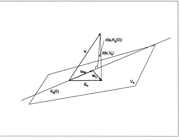
where c' is an independent constant. Figure 3-1 shows schematically the spaces and vectors involved.

1

Suppose now that c' = is not independent of h. Hence, the distance between u and Kh(0) will not decrease at the same rate as d(u, Vh). However, convergence will still occur if d(u, Vh) decreases faster than 3h, though it will not be optimal.

Note that condition (3.18) is a strong guarantee for good convergence properties of our discretization.

The inf-sup condition follows now from (3.18) (see [1] for a nice derivation),

inf sup fn qh div(vh) dQ > > (319)

qhEr~h VhEVh Ijqhjj jjVhjj1

3.1 Incompressible elasticity 25~~~~~~~~~~~~~~~~~~~~~~~~~~~~~~~~~~

If the inf-sup condition is satisfied for a sequence of finite element spaces, then our finite element discretization will exhibit the good approximation properties that we seek, namely, (3.13), (3.16) and (3.18) will all be satisfied.

Figure 3-1: Spaces considered to derive the inf-sup condition

In practice, locking will be present when the potential HI defined in eqn. (3.5) is directly used. To circumvent this phenomenon, the u/p formulation appears as a convenient alternative and the following modified potential is used,

II'(vh) =

G

j

d

+

J

(Ph(div vh))

dQ

(3.20)

d(u,Kh(O)) U

3.1 Incompressible elasticity 26

where Ph(.) is the L2_{-projector operator onto an auxiliary space Qh which we identify}

as a pressure space. The projection operator is defined by,

J(

Invoking stationarity of I'(vh) we obtain

2 G

f

--f(div

J

= f(vh)

=

and we infer from (3.23) that Ph =

Let us now redefine Kh(qh) as

--n Ph(div Uh).

Ki(qh) = {Vh e Vhl/Ph(div Vh) = qh} (3.24)

and the non-locking condition (3.16) becomes,

d(u, Kh(O)) < c d(u, Vh) (3.25)

The inf-sup condition now reads,

inf sup fV qh div(vh) dV

qhEPh(Dh) VhEVh ||qhJ |Vh ll1 (3.26)

where the space Dh in eqn. (3.19) is replaced by Ph(Dh). Therefore, in order to satisfy the inf-sup condition it is crucial how the space Ph(Dh) relates to the displacement

space Vh. Note that Qh always contains Ph(Dh). Choosing Qh smaller renders Kh(O)

larger leaving (3.25) easier to satisfy. However, taking Qh = {0}, we have that

Kh(O) = h, and nothing remains for the incompressibility constraint. According to this, the key is to reduce Qh sufficiently to avoid locking but keeping it as large

3.2 Spurious pressure modes

as possible for reasons of accuracy. On the other hand, using Ph = I (the identity operator) the displacement-based formulation is recovered and the element locks.

Once the inf-sup condition is satisfied, the following error bounds can be shown to hold [18]

IU- uhil < C [ u-uIl + 11(- Ph)(P) ] (3.27)

lip- ,

I(I-Ph)(P)l

3.2 Spurious pressure modes

In this section, we discuss some issues related to the presence of spurious pressure modes.

As mentioned above, in actual finite element discretizations we may well have

Ph(Dh) contained in but not equal to Qh. Therefore, we must consider

inf sup f n qh div(vh) dQ > 0 _ (3.29)

qhEQh VhEVh siqh|| I|Vh|l

instead of (3.26). In case Ph(Dh) = Qh, (3.26) and (3.29) are exactly the same.

In case that the space Qh is larger than the space Ph(Dh), the solution will exhibit spurious pressure modes. They correspond to (non-zero) pressure distributions p, that do not interact with the displacements. Thus, they satisfy,

JQ

Assume now that we are given a pressure distribution iPh which is proposed to be a spurious pressure mode. If Qh = Ph(Dh), there is always a vector v'h such that

3.3 The in f-sup test 28~~~~~~~~~~~~~~~~~~~~~~~~~~~~~~~~~~~~~~~~~~~~~

Ph =-Ph(diVrh) and

- Ph diVVh

dQ

-

d

dQ

> 0

Therefore, since we are testing with qh E Qh, expression (3.29) tests whether any

spurious pressure mode is present. Furthermore, when no spurious pressure modes are present, expression (3.29) tests if condition (3.26) is satisfied.

Spurious pressure modes can lead to large solution errors in case of totally incom-pressible situations or when prescribed displacements are different from zero. Further discussion on this topic can be found in [1],[11],[19].

3.3 The inf-sup test

It is not easy to determine whether a particular finite element formulation satisfies the inf-sup condition and only for a very few number of elements an analytical proof is available. See [1] for a review of existing elements. Thus, the numerical inf-sup test proposed in [11] appears as a very useful tool to predict if a certain discretization is likely to satisfy the inf-sup condition. Such a test can be applied to newly proposed elements and also to discretizations with elements of distorted geometries. However, we understand that this test, when passed, does not assure the satisfaction of the inf-sup condition, but, of course, if the numerical test is not passed that automatically means that the inf-sup condition is not satisfied.

To establish the basis of the inf-sup test, we consider the matrix problem associ-ated with eqns. (3.22) and (3.23) for finite values of ;

33Teif-su tes 29

Ah B Uh Fh

7Th] =

H

V

(3.32)

Bh Th Ph 0

Clearly, from the last equation we have

1 Ph

BhUh

-ThPh

=

=Ph

-T- BhUh

(3.33)

and it follows that -T- 1Bh is the matrix form associated with the linear operator

Ph(div(.)).

We can also write condition (3.26) in terms of nodal quantities instead of the fields. We note that having qh G Ph(Dh) it is always possible to find wh such that

qh Ph(div Wh). Thus, we obtain an all-displacement form of the inf-sup condition

WT Gh Vh inf sup W= h > (3.34) Wh Vh W Gh Wh Vh Sh Vh where

Vh

ShVh

'E

i"1

'~i9

dV

(335)

J

dV

(3.36)

with Sh a symmetric positive definite matrix and Gh a symmetric positive semi-definite matrix.

The key is the evaluation of the inf-sup value of the expression in (3.34). To do that, the following eigenproblem must be considered.

Gh Vh = A Sh Vh

3.3 The inf-sup test 29

3.3 The in f-sup test 30

Let us now call Ap the first non-zero eigenvalue. Then, the inf-sup value is simply /p (see [11]) and we require that for any sequence of meshes this value remain bounded from below by a constant oh > 0.

We can also detect the presence of spurious pressure modes in our formulation. Suppose that we have nu displacement and np pressure degrees of freedom. We should get that AnU-np+l is the first non-zero eigenvalue. Otherwise, spurious pressure modes are present in our finite element discretization.

Summarizing, to perform the inf-sup test it is necessary to design a proper analysis problem and consider a sequence of meshes to evaluate the first non-zero eigenvalue in eqn. (3.37). If the values obtained approach asymptotically a value greater than zero (and there are no spurious pressure modes) the inf-sup test is passed. Even though to pass the numerical inf-sup test does not guarantee that the inf-sup condition is satisfied in all cases, it is a very rigorous test. Results of the numerical inf-sup test applied to existing formulations can be seen in [1]. In chapter 4 we implement this test for our proposed element.

Chapter 4

Development of the element

In this chapter we present a new formulation which shows promise for general com-pressible and incomcom-pressible analysis of solids and fluids. First, we present our pro-posed element which is based on a mixed interpolation of displacements (velocities), pressure and strains (velocity strains). We implement the inf-sup test in section 4.2 and also discuss other possibilities that can be used in the selection of the interpola-tion fields in the last secinterpola-tion.

4.1 The new proposed element

4.1.1

Variational formulation

Let B be a general body in the space with prescribed displacements over the boundary

S, applied tractions over S and Su n Sf = 0. The material response is assumed

to be represented by a polyconvex stored energy function W(x, e), where x indicates material points and E denotes the strain tensor. We can always split the strain tensor into a deviatoric and spherical or volumetric part,

Is' = As t1

f =E- - tr(e)

tr(e')

0

(4.1)

3

-4.1 The new proposed element 32

e = tr(E) (4.2)

where 6 denotes the unit second order tensor.

The stress tensor and the constitutive tensor are given by

a9W(x,,)

W(x,

)

C = Oe0

_OE

0= 2W(x, E) (4.4)

Note that the tensor C as defined in (4.4) is neither isotropic nor constant. More-over, it only depends on the stored energy function W(x, e).

We now assume a physical situation in which volumetric and deviatoric response are uncoupled and by virtue of the kinematic split (4.1) and (4.2) we can rewrite W as a function of E' and E,,. Namely, W(x, c) can be written as

W(x, e) = W'(x, E') + Wv(x, ev) (4.5)

and now

=

aW'(x,

e')

C

9E' 0E'

P W (x e) _ 2Wv(x,,e) (4.7)

P= &ev n ~ =-ke~e

where Tr' is the deviatoric part of the stress tensor and p is the pressure. In the following we will refer to isotropic elasticity with constant material properties. We call C' the stress-strain matrix law and n the bulk modulus. However, because of the generality of the variational principles, our results are applicable to any solid provided the corresponding expression of the stored energy function is used. Moreover, they are also valid even if the material response cannot be uncoupled as assumed in eqn.

4.1 The new proposed element 33

(4.5).

Let us consider the following variational indicator [1]

In*(u,p) = f[

e'. C' E' +

where u denotes the displacement field. The term 7R(u) accounts for the externally applied body forces fB and surface tractions fsf,

%(u) = v U. fB dV ₊

Io

Inspired by the developments given in [51 and [14], we write the strain field as,

Ef

=

qU +

where &9u is the strain corresponding to the displacement field u and e represents an enhancement in the strain field. The deviatoric and volumetric strains are now given by,

E' = 6,U + e Ev = &e₁ + v

Substituting from eqns. (4.11) and (4.12) into eqn. (4.8), we obtain

II(u,

e,

Xp)

=

JV[

(,,

U

+ ).

C'

(u

+

')

(a, u +

Z,)]

dV

- R(u)

Note that we obtain the stress tensor r as

1 p2

2 - (PK (4.8)

(4.9)

4.1 The new proposed element 33

4.1 The new proposed element 34

r = r'

-p

6

(4.14)

where the deviatoric part is

=

C (,u +

)

(4.15)

Invoking stationarity of II we obtain the following governing variational equations,

[6u.

C' ( u +

,)

,,6u p] dV - 67Z(u) = 0

|[hi

*

(,u

)-

0

(4.16)

P (,p

EV))]dV

The first of eqns. (4.16) gives the well-known equilibrium equation and the last one gives the relation between pressure and volumetric strain. Since we know that the stress field cannot be zero under the action of externally applied loads the second equation imposes conditions to the enhanced strain field, which means that it cannot be arbitrarily selected. In fact, for the constant stress field case (patch test) the second of eqns. (4.16) becomes,

r-6EdV

0

(4.17)

which means that the integral of the enhanced strain field must vanish. We will choose our finite element interpolations of the enhanced strain field such that condition (4.17) is satisfied and will refer to this point in more detail in the following section.

4.1 The new proposed element 35

4.1.2

Implementation

The geometry and the displacement field are described using the standard 4-node isoparametric interpolations 4 x = h(r) xi (4.18) {=1 4 u =

Ehi(r)

In these equations, hi are the usual interpolation functions, r indicates the isopara-metric coordinates, and xi and ui are the nodal point coordinates and nodal point displacements, respectively. The deviatoric and volumetric strains corresponding to u are

Y

9_{,u = B'(r) fi (4.20)}

Ou = B.(r) fi (4.21)

where B'(r) and B, (r) are, respectively, the corresponding strain interpolation ma-trices and d contains the nodal point displacements.

The crucial ingredients of the element formulation are the interpolations of the pressure field and the enhanced strain field. As is well known, using the bilinear dis-placement interpolation and no enhanced strain field (that is, using e = 0), the "best"

element is the displacement/constant pressure element (the 4/1 or Q1/P0 element). Any higher order pressure interpolation deteriorates the element performance in al-most incompressible analysis, and even the constant pressure element is not reliable (unless used in certain macro-element patterns). The 4/1 element does not satisfy the inf-sup condition.

We are using the enhancement in the strain field to increase the predictive

4.1 The new proposed element 36

bility of the element in bending and enlarge at the same time the "divergence space" of the element. Based on these thoughts, we propose to use the same interpolation for the pressure as for the displacements, that is

4

p=

Zhi(r)

pi = H(r)

(4.22)

i=1

where the Pi are the nodal point pressure values.

Hence the element will yield a continuous pressure field across the element bound-aries.

With the above displacement and pressure interpolations it is now crucial to select an appropriate strain field e.

Let us define the enhanced strain field interpolation as

C = G(r) a

(4.23)

The matrix G(r) (to be defined in detail) contains functions of r and the vector a contains the internal element parameters.

Using eqns. (4.18) to (4.23) in eqns. (4.16) we obtain the following discrete finite element equations, Kuu, KUQ KU p 1

1a

0

~~K

wherepJ

4.1 The new proposed element 37

K

uu

=

B (r) C' B(r) dV

K

= -J

B

(r) H(r) dV

Kpp = J|-HT(r) H(r) dV Kap = - GV (r) H(r) dV (4.25) K = f

vGIT(r)

and R is the usual load vector.

The final stiffness matrix is obtained by statically condensing out the internal parameters xa at the element level.

The matrix G(r) must satisfy the requirement that the linear system of equations (4.24) be solvable, that is, after elimination of the physical rigid body modes. We also want that the element passes the patch test.

Of course, satisfying these requirements does not assure that we have a stable finite element discretization. However, this solvability condition is necessary and the passing of the patch test indicates whether the element will be useful. Ideally, as mentioned above, we would be able to analytically show that the element formulation satisfies the inf-sup condition for incompressible analysis.

The system of equations (4.24) will be solvable if the matrix Kaa is invertible, which is guaranteed if the columns of the matrix G(r) are linearly independent.

According to our variational principle, the integral of e over the volume of the element

must vanish. Hence, assuming a constant thickness we must have

f

/+ |/+ G(r) J(r) dr =

-

(4.26)

where J(r) is the Jacobian determinant for the transformation from the physical

4.1 The new proposed element 38

coordinates (x,y) to the isoparametric coordinates (r,s).

We will now establish the enhanced strain interpolation defined in eqn. (4.23). Let us consider first a square element of size 2x2. In this case we use G(r) = G*(r),

r 0 0 0 rs

G*(r) 0 s 0 0 0 rs (4.27)

0 0 r s 0 0

Note that the first four columns of G* define the strain interpolations that actually correspond to the incompatible displacement interpolations used in the element of Wilson [14]. The two columns that we add in G*(r) enable the element to pass the numerical inf-sup test given in section 3.3.

If the element is a general quadrilateral we need to transform the strains in the isoparametric coordinate system to the physical coordinate system and we perform this tensor transformation in matrix form,

G(r) - J(r) Xo G*(r) (4.28)

where

_-1

Xo2 Xo2l Xo1Xo21

-1

Xo = Xo2 Xo22 X012Xo22 (4.29)

2Xol 2Xoj 2Xo2 1Xo22 X0 11oX 0 2 2 + X0 12X0 21

and

9x(r)

X oar =o and Jo = Jlr=O (4.30)

Hence, we use in eqn. (4.28) the geometry gradient and determinant evaluated at the center of the element. Since the condition (4.26) is satisfied for the square element,

4.1 The new proposed element 39

the same condition is also satisfied for the element of general geometric shape. We note that, of course, higher order terms can be included in the strain inter-polation matrix G*(r) provided condition (4.26) is satisfied. However, we performed some numerical experimentation which showed that no significant improvements are obtained by including higher-order terms (see section 4.3).

4.1.3

The axisymmetric element

For axisymmetric analysis due to the hoop strain and the presence of the factor xr (r) (the radius expressed as a function of the natural coordinates) in the integrations, some extensions of the above element formulation are needed.

To include an enhancement for the hoop strain we modify the enhanced strain interpolation (4.27). Consider the 2x2 element and the interpolation matrix

G (r) =

0O r s 0 0

Using G (r) condition (4.26) is now violated due to the additional thickness factor xr(r) in the integral and a normalization of the interpolation (4.31) is required.

Let

~ * t

G*(r) = G (r) + G,

(4.32)

i- *

where G, is a correction matrix of constant elements to satisfy eqn. (4.26). Then we obtain

G*(r) = G (r)-.f

(

d

G (r) x(r) dr

(4.33)

4.2 Implementation of the numerical inf-sup test

The matrix G(r) for a general quadrilateral element is then obtained by the trans-formations defined in eqns. (4.28) to (4.30).

4.2 Implementation of the numerical inf-sup test

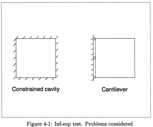
In the numerical inf-sup test we choose an analysis problem and investigate whether the inf-sup values in the finite element solutions of that problem, with increasingly finer meshes, are bounded. We choose the constrained cavity and the cantilever

problem shown in Figure 4-1 to perform our analysis.

/ f/ / / / / /

,//

/ / / / / /

Constrained cavity Cantilever

Figure 4-1: Inf-sup test. Problems considered

We use here the inf-sup condition as written in terms of the nodal quantities (eqn. (3.34)) and solve the eigenproblem given by eqn. (3.37).

The key is the evaluation of the matrices Gh and Sh defined by eqns. (3.35) and (3.36) respectively. To this end we consider the matrix problem that corresponds to

I

4.2 Implementation of the numerical inf-sup test

the variational formulation defined in eqns. (4.16),

Ah

B4

Bh - Th Ph

K

From eqn. (4.24) we can immediately identify,

(Kuu)h (Kua)h Ah = (Ku,)T (KQQ)h BT [ (Kup)h] h (Kp)h Th =

X

Uh ={

:1

Ph = {}

4.2 Implementation of the numerical inf-sup test

R(u)

Fh = (4.40)

0

Gh is now directly obtained from, [11]

Gh = B T 1 Bh (4.41)

Note that externally applied loads and material parameters do not affect the expressions in eqns. (3.35) to (3.37).

The evaluation of Sh must include the fact that we are interpolating not only the displacements but also strains. Making use of Korn's inequality [17], we therefore use instead of the 1-norm that enters in eqn. (3.26) and evaluated in eqn. (3.35), an equivalent norm defined in terms of the components of the strain tensor,

(3 1/2

lV = E II Ej 112 (4.42)

i,j=-1

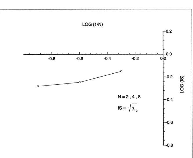
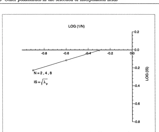
Figure 4-2 shows the results of the test applied to the constrained cavity shown in Figure 4-1. The figure shows that the test is passed. Also, the count of the number of zero eigenvalues, after removal of the physical pressure mode, shows that spurious modes are not present.

The evaluation of the inf-sup value was performed for three uniform meshes in which N=2,4,8 where N is equal to the number of elements per side. IS =

Vp,

4.2 Implementation of the numerical inf-sup test 43 LOG (1/N) I~~~~~~~~~~~~~~~~~~~~~~~~~~~~~~~~~~~~~~~~~~~~~~~ aN , I ,I I I I , , I I I ,I , I , [I I -0.8 -0.6 -0.4 -0.2 0

N=2,4,8

IS=

F/p

0

0

_{_}

Figure 4-2: Results of the inf-sup test for the constrained cavity shown in Figure 4.1. N is the number of elements per side of plate in Figure 4.1 and IS is the calculated inf-sup value

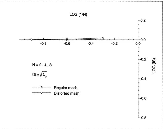
The results of the numerical inf-sup test applied to the cantilever problem shown in Figure 4-1 are shown in Figure 4-3. We performed the test over a regular and a distorted mesh. The test is passed in both cases. It can be inferred from the picture that the distortion of the elements does not affect appreciably the results.

4.3 Other possibilities in the selection of interpolation fields LOG (1/N) -UZ -0.0 0 -0.2

*

0

₀

N=2,4,8

IS =/p

Figure 4-3: Results of the inf-sup test for the cantilever problem shown in Figure 4.1. N is the number of elements per side of plate in Figure 4.1 and IS is the calculated inf-sup value

4.3 Other possibilities in the selection of

interpo-lation fields

Since we are interpolating both, the strain and pressure fields, many possibilities are open to select their approximations. Of course, once we choose the interpolations we 44

4.3 Other possibilities in the selection of interpolation fields

do not know a priori whether they will work or not. However, based on theoretical knowledge we can predict if a certain selection will fail or not. Other cases are not so obvious and their usefulness is determined by numerical experience.

We want to discuss in this section different approaches that we have investigated and the thoughts that guided us to arrive to our final results.

The main objective is to develop a new element that satisfies the relevant inf-sup condition. The numerical inf-inf-sup test presented in chapter 3 and implemented in section 4.2 when strain interpolations are used, is employed as a tool to predict whether the element is likely to satisfy the inf-sup condition. Ideally a mathematical proof is available.

To establish the approximations for our element, we focus our attention on some well-known elements like the 4/1, 4/3, 9/3 and 9/4-c elements. These elements fall in the context of the u/p formulation and analytical proofs that determine whether they satisfy the inf-sup condition are available [1],[10] . The first two do not satisfy the inf-sup condition. The 4/1 element presents spurious pressure modes under certain modeling conditions while in the 4/3 element the pressure space is too large to satisfy the incompressibility constraint. On the other hand, for the last two, the inf-sup condition is satisfied. Also, nine-node elements present an additional advantage, namely, they give exact results under bending action even if distorted elements are used.

4.3.1

The enhanced strain field interpolation

Since it is the strain field that enters in the potential II defined in eqn. (4.8), we begin our analysis by comparing the strain field obtained with the four-node and the nine-node square elements (note that the Jacobian matrix is constant in this case). Let us first construct the B matrix for the four-node square element. By inspection, we determine that it spans the same space as the column space of the following linear operator

4.3 Other possibilities in the selection of interpolation fields

1 0 0 s 0 0 0

B (r)

0 1 0 0 r 0 0

(4.43)

0 0 1 0 0 r s

We now consider the space generated by the B matrix obtained from the nine-node displacement interpolations. To obtain this space, it is necessary to add the following columns to B1

r 0 rs 0 0 s2 0 0 0 rs2 0 0 0

G1(r)= 0 s 0 rs 0 0 r2 0 0 0 sr2 0 0 (4.44)

0 0 0 0 rs 0 0 r2 s 2 0 0 sr2 rs2

We remark that in the case of distorted elements the Jacobian matrix is no longer constant and the above matrix entries are changed.

Let us now concentrate on expression (4.44). We could use G1 as our enhanced

strain field interpolation (eqn. (4.27)). However, we can immediately appreciate that G₁ does not satisfy condition (4.26) which implies that the patch test will not be passed. Clearly, the integral over the volume of the element of terms like r2 _and

s2 is not zero. Deleting the columns in G1 that contain those terms will leave us

with condition (4.26) satisfied at the price of loosing the capabilities of the nine-node ment. Therefore, we have

r 0 rs 0 0 rs2 0 0 0 ) = 0 s 0 rs 0 0 sr2 0 0 (4.45) 0 0 0 0 rs 0 0 sr2 rs2 ' -,, , 46

4.3 Other possibilities in the selection of interpolation fields

Using this operator as our enhanced strain interpolations requires the inversion of a 9x9 matrix to condense out the internal parameters a. Furthermore, exact inte-gration requires the use of a 3x3 quadrature rule which would make the element very expensive. The computational cost can be reduced further by noting that numerical results are not much affected if we neglect the last four columns in (4.45). However, the resulting enhanced strain interpolation operator still differs from the one that we have defined in (4.27). Our numerical experience showed that better results are obtained if we use (4.27) when distorted elements are present in the model. Thus, we finally use,

r 0 0 0 rs 0

G*(r) 0 s 0 0 0 rs (4.46)

0 0 r s 0 0

If the last two columns of G* are not used the incompatible element of Wilson [14] is recovered. We would like to make some comments at this point regarding the use of

r 0 0 0

G*(r) = 0 s 0 0 (4.47)

0 0 r s

First of all, the patch test is passed since G*, satisfies condition (4.26). Let us now consider the cantilever problem that we use in Section 4.2 to perform the numerical inf-sup test. We clearly have in this model, if we use (4.47), that n > np which is

a necessary condition for a discretization to be stable but not sufficient. In fact, the numerical inf-sup test is not passed. A spurious pressure mode is present and the value of the first non-zero eigenvalue is not bounded from below as shown in Figure

4-4.

4.3 Other possibilities in the selection of interpolation fields

Figure 4-4: Results of the inf-sup test using the strain interpolations defined in eqn. (4.47). N is the number of elements per side of plate in Figure 4.1 and IS is the calculated inf-sup value

4.3.2

Pressure interpolations. Internal degrees of freedom

Constant pressure interpolation

The pressure is defined to be constant throughout the element and the space Qh

defined in chapter 3 is the space of constant functions. In the context of the u/p formulation the equivalent element is the 4/1 or Q1-P0 element. We know that the 4/1 element has a spurious pressure mode. However, due to the fact that we have an

LOG (1/N) . I I I I . I I J I I I I I I I I I I I . -0.8 -0.6 - -0.2 0 N=2,4,8 IS= p -U.:, -0.0

0

0

4.3 Other possibilities in the selection of interpolation fields

enhancement in the strain interpolations, we may expect that the spurious pressure modes be filtered out in the model.

Let us define now the following operators,

1

I'

= I -

6®6

(4.48)

3

I = § 5 (4.49)

where I is the unit fourth-order tensor with components Iijkl = {6ikSjt + 6i1Sjk}.

They are linear operators that map a second order tensor into its deviatoric and spherical part respectively. Thus, we can apply these operators to each column of our enhanced strain operator (note that each column of G* is a second order tensor by itself) to obtain G' and G,.

Clearly, the resulting operators G' and Gv will both satisfy similar conditions to (4.26), namely,

+1 +1

f f

G'(r)J(r)dr =

0

(4.50)

-1 1

fJ

Jf

Although we have enhanced the strain field, we will show that, as for the 4/1 element, a spurious pressure mode will appear in certain situations and the inf-sup condition is not satisfied. To demonstrate that a spurious pressure mode is present we need to prove that given a (non-zero) pressure distribution p we have

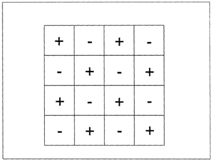
jp di Vh dQ = Vvh Vh (4.52) Let us consider a finite element discretization like the one shown in Figure 4-5 with the pressure distribution (checkerboard) indicated in Figure 4-6. In this model 49

4.3 Other possibilities in the selection of interpolation fields

all displacements along the boundary are set to zero.

Figure 4-5: Spurious pressure modes. Element discretization

Figure 4-6: Spurious pressure modes. Checkerboard distribution

Over each element we have

50 / /_{/11 1} -? / / / / / / / / / /

+ =

+ =

=

-

-

=

-

4.3 Other possibilities in the selection of interpolation fields

div Uh = v = Oev + 'ev

ev = Gv

a

fa, Pe div uhdQe = Pe Jf(aev + v) de

= e

fn,-(&cu

+

G a) de

fne

If a patch of four elements is considered, for the displacement ui shown in Figure 4-7 we have,

Jn

p div

dQ

(1) + pe)

+

The same holds true when any displacement vi is considered. Therefore, the rela-tion (4.52) is satisfied for any nodal point displacement when the pressure distriburela-tion is the indicated checkerboard pressure.

We conclude that when using strain interpolations with the pressure field constant over the element the satisfaction of the inf-sup condition is not possible.

where

and

4.3 Other possibilities in the selection of interpolation fields

Figure 4-7: Spurious pressure modes. Patch of four equal elements

Linear pressure interpolation

We now discuss the possibility of using a linear pressure interpolation with internal degrees of freedom, that means, they can be condensed out at the element level. The pressure interpolation in this case is given by

= 1 + 2 r + 3 s (4.57)

The space Qh is defined as

Qh =

{1,r,s}

We can immediately see that, according to what we have discussed for the con-stant pressure interpolation, the first column of Kap is zero. The other two columns are different from zero and they add some extra terms that contribute to improve

G1 ~~~0 p p pi p ._Pe PP4 52