Dynamic prediction of terminal-area severe convective weather penetration

Dynamic Prediction of Terminal-Area Severe

Convective Weather Penetration

by

Daniel Schonfeld

B.S., United States Air Force Academy (2013)

Submitted to the Sloan School of Management

in partial fulfillment of the requirements for the degree of

Master of Science in Operations Research

at the

MASSACHUSETTS INSTITUTE OF TECHNOLOGY

June 2015

c

Massachusetts Institute of Technology 2015. All rights reserved.

Author . . . .

Sloan School of Management

May 8, 2015

Certified by . . . .

Hamsa Balakrishnan

Associate Professor of Aeronautics and Astronautics

Thesis Supervisor

Accepted by . . . .

Patrick Jaillet

Dugald C. Jackson Professor

Department of Electrical Engineering and Computer Science

Co-director, Operations Research Center

Dynamic Prediction of Terminal-Area Severe Convective

Weather Penetration

by

Daniel Schonfeld

Submitted to the Sloan School of Management on May 8, 2015, in partial fulfillment of the

requirements for the degree of Master of Science in Operations Research

Abstract

Despite groundbreaking technology and revised operating procedures designed to improve the safety of air travel, numerous aviation accidents still occur every year. According to a recent report by the FAA’s Aviation Weather Research Program, over 23% of these ac-cidents are weather-related, typically taking place during the takeoff and landing phases. When pilots fly through severe convective weather, regardless of whether or not an acci-dent occurs, they cause damage to the aircraft, increasing maintenance cost for airlines. These concerns, coupled with the growing demand for air transportation, put an enormous amount of pressure on the existing air traffic control system.

Moreover, the degree to which weather impacts airspace capacity, defined as the num-ber of aircraft that can simultaneously fly within the terminal area, is not well understood. Understanding how weather impacts terminal area air traffic flows will be important for quantifying the effect that uncertainty in weather forecasting has on flows, and developing an optimal strategy to mitigate this effect.

In this thesis, we formulate semi-dynamic models and employ Multinomial Logistic Regression, Classification and Regression Trees (CART), and Random Forests to accu-rately predict the severity of convective weather penetration by flights in several U.S. airport terminal areas. Our models perform consistently well when re-trained on each individual airport rather than using common models across airports. Random Forests achieve the lowest prediction error with accuracies as high as 99%, false negative rates as low as 1%, and false positive rates as low as 3%. CART is the least sensitive to differences across airports, exhibiting very steady performance. We also identify weather-based fea-tures, particularly those describing the presence of fast-moving, severe convective weather within the projected trajectory of the flight, as the best predictors of future penetration. Thesis Supervisor: Hamsa Balakrishnan

Acknowledgments

I would like to thank my advisor, Professor Hamsa Balakrishnan, for her support and guidance throughout this project. Thanks to ICAT alum Yi-Hsin Lin for getting me up to speed with the data used in this thesis and answering any and all questions about her research. Thanks also to my fellow ORC students and friends, particularly Jack, Zeb, Kevin, and Virgile for their help at various stages of the project and for listening to me ramble about weather penetration and technical support. Finally, I would like to thank my family for encouraging me to pursue a graduate degree, and for cheering me on throughout the process.

Contents

1 Introduction 18

1.1 Background . . . 19

1.1.1 Convective Weather Avoidance Model (CWAM) and Weather Avoid-ance Fields (WAFs) . . . 19

1.1.2 Defining “Severe Convective Weather” . . . 21

1.1.3 Defining the “Terminal Area” . . . 22

1.1.4 Terminal Area Operations . . . 23

1.2 Thesis Contribution . . . 25

1.3 Thesis Organization . . . 26

2 Overview of Data 27 2.1 Weather Data . . . 27

2.1.1 Vertically Integrated Liquid (VIL) . . . 28

2.1.2 Echo Tops . . . 30

2.1.3 Case Days . . . 31

2.2 ETMS Database . . . 32

2.2.1 Verifying ETMS Trajectory Data for Model Dataset . . . 33

2.3 ASPM Database . . . 37

3 Feature Identification 37 3.1 Three Separate Models . . . 37

3.2 Dynamic Nature of Models . . . 39

3.3 Weather-Based Features . . . 42

3.3.1 Measuring Severity of Weather . . . 44

3.3.2 Measuring Movement of Weather . . . 45

3.4 In-Flight Features . . . 49

3.4.1 Time Spent Within Terminal Area . . . 50

3.4.2 Flight Behavior Within Terminal Area . . . 51

3.4.3 Positioning Within Terminal Area . . . 55

3.5 Behavior of Other Pilots in the Terminal Area . . . 57

3.5.1 Are Flights Ahead Penetrating Severe Convective Weather? . . . 58

3.5.2 Behavior of Flights in the Opposite Sequence . . . 59

3.5.3 Follow the Leader . . . 60

3.5.4 Feature Summary . . . 62

4 Predictive Modeling of Pilot Behavior 64 4.1 Defining the Dependent Variable . . . 64

4.2 Defining our Model Dataset . . . 68

4.3 Predictive Methods . . . 69

4.3.1 Multinomial Logistic Regression . . . 70

4.3.2 Classification and Regression Trees (CART) . . . 70

4.3.3 Random Forests . . . 72

4.4 Model Results . . . 73

4.4.1 Model 1 Results . . . 74

4.4.2 Model 2 Results . . . 76

4.4.3 Model 3 Results . . . 81

4.4.4 Summary of ORD Results . . . 85

4.5 Testing Our ORD Models on Other Airports . . . 86

4.5.1 Selecting Airport Pairings for Common Model Experiment . . . 87

4.5.2 Comparison of Results . . . 89

4.5.3 Insight from Pairings Experiment . . . 91

4.6 Sensitivity of Models . . . 92

5 Case Studies and Pilot Experience 94 5.1 Takeaways from Pilot Interviews . . . 95

5.1.1 Weather Radar and Forecasting Technology in the Cockpit . . . 95

5.1.2 Deviation from the Filed Flight Path . . . 95

5.1.3 Impact of Convective Weather on Departures . . . 96

5.1.4 Impact of Convective Weather on Arrivals . . . 97

5.1.5 Summary of Interview Takeaways . . . 98

5.2 Case Studies . . . 98

5.2.1 Theme 1: Pilots Try to Avoid Storm Cells . . . 99

5.2.2 Theme 2: Arrivals Have a Tougher “Go-of-It” . . . 101

5.2.3 Theme 3: Weather Is Unpredictable . . . 102

5.2.4 Case Study Wrap-Up . . . 104

6 Conclusions and Future Work 105 6.1 Thesis Summary and Conclusions . . . 105

6.2 Ideas for Future Work . . . 106

6.2.1 Expand Model Datasets . . . 106

6.2.2 Incorporate Weather Forecasts . . . 107

6.2.3 Additional Weather Features . . . 107

List of Figures

1.1 Example of WAF lookup table [15]. . . 20

1.2 Map of Chicago O’Hare arrival fixes. O’Hare’s TRACON is outlined in blue [14]. . . 24

2.1 Example of a VIL image from June 13, 2008, at 0000Z [14]. . . 29

2.2 Example of an ET image from June 13, 2008, at 0000Z [14]. . . 31

3.1 Terminal area intervals for Model 1. . . 39

3.2 Distribution of Penetrations by Distance from ORD . . . 40

3.3 Projected flight trajectory looking 10 km out with swath width of 55 degrees. Angles and distances are not exactly to scale. . . 43

3.4 Calculation of weather-based feature that measures severity. . . 44

3.5 Distribution of penetration entries by severe weather coverage within the tra-jectory projection. . . 45

3.6 Calculation of weather-based features that measure movement. . . 46

3.7 Example of flanking metric calculations with the number of red cells represent-ing “flankcount” and the standard deviation of the degree values representrepresent-ing “FlankingValue”. . . 48

3.8 Plot of Altitude vs. Distance from Takeoff for departure trajectories on July 2nd that penetrated severe convective weather. . . 51

3.9 Plot of Altitude vs. Distance from Takeoff for departure trajectories on July 2nd that took place during a weather impact but did not penetrate. . . 52

3.10 Plot of Altitude vs. Distance from Takeoff for departure trajectories on June 10th with no weather impact. . . 52

3.11 Plot of arrival flight executing a trombone maneuver at ORD. The red dots represent the trajectory points and the nose of the plane is represented by the red circle. . . 54

3.12 Example of Model 3 distance metric calculations with point-to-point distance measured in kilometers representing “DistfromLanding” and angular distance

measured in degrees representing “CircleDistfromLanding”. . . 57

3.13 Example of “follow-the-leader” behavior by departures in the West sector of the ORD terminal area. . . 61

4.1 Distribution of VIL and Echo Top values for arrival and departure penetra-tions within the ORD terminal area. . . 67

4.2 Model 1 ORD CART Output . . . 75

4.3 Model 2 ORD CART Output . . . 78

4.4 Model 3 ORD CART Output . . . 82

4.5 Map of Top 30 Penetration Airports . . . 87

5.1 Example of avoidance behavior by arrivals in the Southwest sector of the ORD terminal area on July 9, 2008 at 001730Z. . . 99

5.2 Example of unexplained penetration behavior by a departure in the Northwest sector of the ORD terminal area on July 8, 2008 at 061730Z. . . 100

5.3 Both departures and arrivals affected by weather in the West sector of the ORD terminal area on July 2, 2008 at 222500Z. . . 101

5.4 Ground stop is issued due to weather covering the airport on July 2, 2008 at 223230Z. . . 102

5.5 Arrivals executing approach and landing maneuvers amidst severe weather in the Northwest sector of the ORD terminal area on August 22, 2008 at 173000Z.103 5.6 Concentration of VIL level 6 pixels forms in the middle of the arrival approach path in the Northwest sector of the ORD terminal area on August 22, 2008 at 174000Z. . . 104

5.7 Arrivals begin to circumvent the storm cell as it moves west to east in order to maintain the approach path in the Northwest sector of the ORD terminal area on August 22, 2008 at 175730Z. . . 105

List of Tables

2.1 VIL Level Cutoffs . . . 29

2.2 List of severe convective weather penetration periods within the ORD terminal area during summer 2008. . . 32

3.1 Summary of Model Features . . . 64

4.1 VIL Point Assignment . . . 65

4.2 Echo Top Point Assignment . . . 65

4.3 Dependent Variable Cutoffs . . . 66

4.4 Breakdown of frequencies of each severity level for Models 1, 2, and 3. . . 68

4.5 Model 1 Performance Results . . . 74

4.6 Model 1 CART Feature Importance Values . . . 75

4.7 Model 1 Random Forests Feature Importance Values . . . 77

4.8 Model 2 Performance Results . . . 78

4.9 Model 2 CART Feature Importance Values . . . 79

4.10 Model 2 Random Forests Feature Importance Values . . . 80

4.11 Model 3 Performance Results . . . 81

4.12 Model 3 CART Feature Importance Values . . . 83

4.13 Model 3 Random Forests Feature Importance Values . . . 84

4.14 Airport Pairings . . . 88

4.15 Comparison of Model 1 performance results for the re-training vs. airport pairing methods. For predictive methods, ”MR” represents Multinomial Lo-gistic Regression, ”Tree” represents CART, and ”RF” represents Random Forests. Regarding performance metrics, “Acc” represents the prediction ac-curacy. “FN 1” represents the first false negative rate defined, “FN 2” rep-resents the second false negative rate, and “FP” reprep-resents the false positive rate. . . 89

4.16 Comparison of Model 2 performance results for the re-training vs. airport pairing methods. . . 90 4.17 Comparison of Model 3 performance results for the re-training vs. airport

pairing methods. . . 90 4.18 Comparison of Model 1 performance results for variable subsets. For

pre-dictive methods, ”MR” represents Multinomial Logistic Regression, ”Tree” represents CART, and ”RF” represents Random Forests. Regarding perfor-mance metrics, “Acc” is the proportion of interval entries for which the model predicts the correct severity level. “FN 1” examines how often the models pre-dict a severity level lower than the actual severity level that occurred. “FN 2” examines how often the models predict a severity level of 0 when in fact the severity level was greater than 0. “FP” measures the proportion of interval entries for which the model predicts a severity level greater than 0 when in fact the severity level was 0. . . 93 4.19 Comparison of Model 2 performance results for variable subsets. . . 93 4.20 Comparison of Model 3 performance results for variable subsets. . . 94

1

Introduction

The increase in demand for air travel in the United States has resulted in an increase in congestion and delays in the National Airspace System (NAS), making the system more susceptible to weather disruptions. Convective weather can close airports, degrade capacity for acceptance/departure, hinder or stop ground operations, and make operations inefficient in general [13]. These disruptions are particularly impactful during summer months, when travel demand is high and there is frequent convective weather activity (i.e. thunderstorms) across the United States [16]. Furthermore, the desire to sustain and meet air travel demand sometimes forces pilots into situations in which they are unable to avoid weather penetration, and controllers into situations in which they are unable to prevent it. When a pilot penetrates convective weather, intentionally or unintentionally, he/she not only puts those onboard in danger but also causes damage to the aircraft, resulting in lost revenue and excessive maintenance costs.

Moreover, although it is clear that convective weather reduces airspace capacity and results in inefficient flying, the degree to which capacity is reduced and air traffic flows are affected as a result of weather is not clear. The re-routing of planes within the terminal area, initiated by either the pilot or air traffic controller, reduces airspace capacity and increases controller workload. Existing research into the types and severity of weather that cause re-routing/deviation typically treats all flights as equal [14], failing to differentiate between specific aircraft types, regional vs. international flights, departures vs. arrivals, and other flight categories. This thesis takes a different approach by exploring operational factors that may differentiate pilot behavior as well as weather-based factors that indicate future penetration within the terminal area.

1.1

Background

In this thesis, we rely heavily on research previously conducted by Yi-Hsin Lin at the MIT International Center for Air Transportation (ICAT). Lins work built on the Convective Weather Avoidance Models (CWAM) developed at MIT Lincoln Laboratories. The CWAMs produce Weather Avoidance Fields (WAF), which identify the areas impenetrable to aircraft as a result of weather. The following subsections below will briefly describe the succession of CWAMs and WAF, and then explain why we chose to define severe convective weather differently than Lin.

1.1.1 Convective Weather Avoidance Model (CWAM) and Weather Avoidance Fields (WAFs)

Rich DeLaura and his team at MIT Lincoln Laboratories developed the CWAM in response to increasing delays in the NAS caused by thunderstorms. The CWAM provides decision support tools for air traffic controllers to aid them in determining the impact of weather on existing traffic, devising a tactical response to mitigate the impacts of weather, predicting the effects of a particular routing strategy, and predicting updated arrival times for flights sub-jected to regions of convective weather [7]. The CWAM achieves this by analyzing planned and actual trajectories as well as a variety of weather indicators to predict enroute flight deviations due to convective weather.

There are several versions of the CWAM. The first model (CWAM1), which focused on enroute flights, was developed in 2006 based on 800 trajectories over five different days in the Indianapolis (ZID) and Cleveland (ZOB) “super sectors” [7]. The study took into account the following three weather indicators that will be discussed in more detail in Chapter 2: VIL (measure of precipitation intensity), echo tops (storm height), and lightning strike counts. The second version (CWAM2), which also focused on enroute flights, was developed in 2008 and expanded the number of flights in the dataset to about 2,000 by adding the Washington

D.C. “super sector” [8]. It also considered additional weather factors such as vertical storm structure and vertical and horizontal storm growth to help decrease CWAM1’s prediction error rate. In 2010, the release of CWAM3 refined earlier models to improve detection of non-weather related deviations, such as shortcuts, and further expanded the dataset to about 5,000 flights [5]. Most recently, MIT Lincoln Laboratories developed a version of the CWAM specific to low-level flights within the terminal area, which typically operate below the tops of convective weather and have slightly different operational constraints [5]. The terminal area CWAM is calibrated based on historical pilot behavior during weather encounters near the destination airport.

All versions of the CWAM return the probability of deviation for a pilot encountering a particular set of weather conditions. This output, commonly referred to as the Weather Avoidance Field (WAF), is a probability lookup table: for any given echo top height and local VIL coverage, the model returns a probability of pilot deviation on a pixel-by-pixel basis [14, 15]. An example of this lookup table can be seen in Figure 1.1. The main advantage of using WAF over the raw VIL/ET metrics is that WAF eliminates much of the light rain that has little to no effect on aviation and accounts for the frequency of lightning strikes within each pixel [14].

The principal difference between the enroute and terminal area CWAMs is the primary determinant of pilot deviation. For the enroute airspace model, the difference in altitude between the flight and the echo top height served as the primary determinant [7]. In contrast, the fractional VIL coverage of Level 3 or above within a specified kernel of the flight trajectory served as the primary determinant of deviation in the terminal area model [5]. This makes sense because pilots can overfly weather during the enroute phase flight, but due to the low altitudes necessary for descent/ascent, pilots typically cannot overfly weather in the terminal area. Therefore, the WAF for enroute flights is fundamentally different than WAF for ascending/descending flights.

1.1.2 Defining “Severe Convective Weather”

A question which naturally arises is how to quantitatively define “severe convective weather”. Lin defined it as WAF levels of 80 or above. WAFs of 80 or above can be interpreted as when a pilot has a greater than 80% chance of actually penetrating Level 3 VIL or above with flight altitude below the corresponding echo top value [14]. In contrast, we chose not to use WAF to classify severe convective weather for a variety of reasons. First, WAF reflects the probability that a pilot will deviate rather than explicitly describing weather conditions like VIL and echo top do. Second, since some low-level VIL pixels will correspond to high WAFs simply because of proximity (within 4 km kernel) to higher VIL levels, it is possible that pilots flying through high WAFs are not actually penetrating severe convective weather at all. At the other end of the spectrum, WAF is low in situations where pilots have no chance of deviating because they are surrounded by severe convective weather. Third, terminal WAF does not account for each individual flights altitude relative to echo top height [14], so it is unclear whether or not the flight is above or below the storm. Lastly, WAF is not consistent: a VIL/ET combination that constitutes a WAF of 80 on one case day does not always translate to a WAF of 80 on another case day. For example, on August 4, 2008, the

WAF model fails when none of the departures that we classify as severe convective weather penetrations have WAF of 80 or above during their entire ascent. Thus, we will define severe convective weather as pixels with VIL Level 3 or above and flight altitude below echo top height.

In our analysis, penetration occurs when pilots taking off from or landing at Chicago O’Hare International Airport (ORD) fly through severe convective weather. This is an important distinction because there are several airports within or just outside the ORD terminal area, which we will thoroughly define in the following section. We do not examine penetrations that take place while departing from or landing at one of these nearby airports. Furthermore, we focus on ORD flights in our analysis because O’Hare is considered one of the worst airports in the U.S. for severe convective weather, with an average of 38 thunderstorm days per year [10]. Since the overwhelming majority of these thunderstorm days occur during the summer months, we will focus on flights that occur in June, July, and August. In the flight database used for this research, O’Hare accounts for the highest number of penetration flights as well as overall penetration entries (i.e. one flight can penetrate multiple times) of any airport in the continental U.S.

1.1.3 Defining the “Terminal Area”

This thesis focuses on pilot behavior within a region near the airport we call the terminal area. The dimensions of this region are not precisely defined, varying from airport to airport. Most major airports have Terminal Radar Approach Control (TRACON) facilities, which serve the airspace immediately surrounding the airport. Using the TRACON boundary is one possible definition. However, TRACONs can vary in size and shape just like terminal areas, and a simpler, more general definition is desirable. To devise the best definition, we must consider what characteristics define the terminal area and why pilot behavior in this region might be different from pilot behavior during the enroute portion of the flight.

The primary difference is that aircraft trajectories are far more constrained both vertically and horizontally within the terminal area. Enroute flights can frequently overfly or deviate around convective weather, whereas a flight in its ascent or descent sequence will most likely be flying below the storm with limited ability to deviate due to the high level of congestion and standardized trajectories in the terminal area.

In this thesis, we define the ORD terminal area for arrivals to be the circle of radius 180 km around the airport, and for departures a circle of radius 150 km around the airport. The specific radii of the terminal areas for arrivals and departures were determined based on when arrivals begin their descent sequence and when departures end their ascent sequences. A 180 km radius was chosen for arrivals because this is the distance at which aircraft begin to continuously decrease their altitude. A 150 km radius was chosen for departures because this is the distance at which aircraft begin to stop continuously increasing their altitude and start leveling off for the enroute portion of the flight. Within these radii, flights are below all non-negligible storm echo tops and cannot overfly the convective weather. Using a circular region simplifies analysis by allowing the region to be broken up into eight equally spaced sectors, each corresponding to cardinal or intermediate directions. At ORD, departures typ-ically take off in the four cardinal direction sectors (North, South, East, West), and arrivals typically land in the four intermediate direction sectors (Northeast, Northwest, Southeast, Southwest).

1.1.4 Terminal Area Operations

The airspace contained within the terminal area can be subdivided into sectors controlled by individual air traffic controllers. Control of aircraft as they fly between these sectors is handed off between the air traffic controllers. The controllers are responsible for maintaining the separation of aircraft, through voice radio communication and aircraft position tracking, and providing real-time information to aircraft such as weather conditions near the airport

[14]. Hence pilots must obtain approval from these controllers to deviate from their filed flight plan.

The airspace capacity of a sector can vary depending on the complexity of flow patterns within the sector or other conditions such as the presence of convective weather. Each flight must follow a Standard Instrument Departure (SID) when departing an airport and a Standard Terminal Arrival Route (STAR) when arriving [16]. These routes are specified by a sequence of waypoints, or fixes, along with rules governing the speed, heading, and altitude of aircraft at certain waypoints [16]. Each airport has multiple STARs and SIDs; the assignment of an aircraft to specific routes is a function of its origin (or destination), aircraft type, runway restrictions, and load balancing of runways [16]. One of the most common terminal area layouts, as seen at Chicago O’Hare, is the four cornerpost configuration, in which airspace is divided into four arrival sectors alternating with four departure sectors. Figure 1.2 contains a diagram of a four cornerpost configuration.

1.2

Thesis Contribution

As mentioned in the Introduction, this thesis relies heavily on the research completed by Yi-Hsin Lin during her time at MIT ICAT. In order to determine the best predictors of severe convective weather penetration, Lin employed models that predicted the maximum WAF penetrated by pilots of arriving aircraft during the descent phase [14]. Her models built upon the WAF model by incorporating operational factors, such as prior delays and existing congestion in the terminal airspace, in addition to weather-based factors. Her best model accurately predicted penetration 90% of the time [14]. She found that weather-based and stream-based features were the most predictive of severe convective weather penetration. In particular, pilots were more likely to penetrate severe convective weather when they were part of a stream following other pilots that crossed through weather and less likely when they were pathfinders leading a new stream [14]. This implies that re-routing around weather is still often based on reported events to air traffic controllers rather than preemptive action based on forecasts [14]. Furthermore, Lin found that pilots were more likely to penetrate severe convective weather closer to the airport because, intuitively, there is less ability to deviate from the flight path upon approach.

Our model is fundamentally different than Lins first and foremost in its definition of severe convective weather, as we examine the raw weather metrics that make up WAF rather than WAF itself. Applying this revised definition, our model dynamically predicts the severity of pilot penetration at several checkpoints throughout the ascent and descent phases for both departures and arrivals respectively. Thus, the features (or predictors) in our model are more specific to the trajectory of the flight and its location relative to the airport. Our best models accurately predict the severity of penetration over 98% of the time with a false negative rate of less than 1% and a false positive rate of less than 3%. Furthermore, the models reveal that the presence of severe convective weather within a specified distance from the projected trajectory of the flight is the best predictor of future penetration. Nonetheless,

the behavior of other flights nearby is still moderately correlated with penetration behavior in the terminal area. If flights close by, whether they be departures or arrivals, are penetrating, it is highly likely that the flight of interest will also penetrate severe convective weather in future time steps. Additionally, we found that the longer amount of time flights spend within the terminal area, the more likely they are to penetrate severe weather. This may seem counterintuitive at first because flights that try to deviate around weather often experience longer flight times. On the other hand, spending more time in the air subjects the flight to more opportunities for severe weather penetration. Lastly, after running our models on several U.S. airports in addition to ORD, we found that our models consistently perform well when re-trained on each individual airport rather than using common models across airports. This held true even among airports in the same region of the continental U.S.

1.3

Thesis Organization

Due to the limited number of time periods plagued by severe convective weather in our research data set, we will present a combination of predictive modeling, case studies, and pilot observation to better understand pilot behavior within the terminal area during severe convective weather scenarios. Chapter 2 discusses the data sources for this study. These include weather data from MIT Lincoln Laboratories, trajectory data from the Volpe Na-tional Transportation Center, and flight information maintained by the Federal Aviation Administration (FAA).

Chapter 3 describes the features included in our predictive models for both arrivals and departures. These features can be classified into three categories: weather-based, in-flight, and features that capture the behavior of other pilots flying in the terminal area simultane-ously.

Chapter 4 describes the three types of predictive models used in this study and the results obtained from employing them. Multinomial Regression was used for its ability to handle well

categorical, dependent variables of more than two classes and independent factor variables. Classification and Regression Trees (CART) were chosen due to their transparency/inter-pretability, applicability to relatively small sample sizes, and ability to weigh the relative importance of features. Random Forests were explored as an extension to CART with an extremely high level of randomness, facilitating the discovery of patterns not detected by CART.

Chapter 5 presents the case studies explored and commonly observed themes of pilot behavior, highlighting scenarios in which pilots penetrated severe convective weather within the terminal area. Along with observations from pilots regarding terminal area procedures during severe convective weather, these case studies will help to verify, or sometimes disprove, model results in order to determine which features truly best predict penetration.

Finally, Chapter 6 discusses the implications of this thesis and plans for future work.

2

Overview of Data

Three main data sources were used in this thesis: weather data from MIT Lincoln Labo-ratories, trajectory data from the Enhanced Traffic Management System (ETMS) database provided by the Volpe National Transportation Center, and airport information from the FAAs Aviation System Performance Metrics (ASPM) database.

2.1

Weather Data

Prior to 2006, there existed a range of competing weather forecasts for aviation that led to a great amount of inconsistencies and confusion in critical air traffic management situa-tions [14]. In response to this highly inefficient and complicated system, the FAA’s Aviation Weather Research Program (AWRP) established the Consolidated Storm Prediction for Avi-ation (CoSPA) program to integrate the different forecast systems into one reliable, accurate system [3]. CoSPA features collaboration from a variety of different organizations including

MIT, NCAR, NOAA, NWS, NASA, and DoD [3]. These organizations, collectively, aim to improve and integrate existing prototype products such as the Corridor Integrated Weather System (CIWS) and the Integrated Terminal Weather System (ITWS) [3].

MIT Lincoln Laboratory is at the forefront of this effort with its tactical (0-2 hr) storm forecasting and has successfully harnessed high-resolution, real-time weather data that ac-curately depicts the severity of storm cells [3]. Through the integration of multiple sensor data sources, including radar (NEXRAD, TDWR, Canadian), satellite imagery, and surface observations, Lincoln Labs has produced Vertically Integrated Liquid (VIL) and echo top maps of the entire continental United States with 1 X 1 km pixel resolution updated every 2.5 minutes [14]. These maps, or matrices of pixel-by-pixel values, will serve as the main weather inputs considered in this thesis and will be described in detail in the following sec-tions. MIT Lincoln Laboratories provided us with weather maps for 14 days in summer 2008. They also provided us with software scripts necessary for converting between latitude/longi-tude and matrix coordinates in each weather image using the Lambert azimuthal equal area projection.

2.1.1 Vertically Integrated Liquid (VIL)

VIL is a measure of the amount of moisture in a vertical column of the atmosphere and is typically used to indicate areas experiencing heavy rain or hail as well as identify potential supercells and downbursts [7]. VIL helps to avoid false alarms by extending to high altitudes and looking at storm cells as a whole instead of just their effect at low altitudes [14]. The raw pixel-by-pixel data provided by MIT Lincoln Laboratories measures VIL on a 0-255 scale. The VIL maps divide these raw values into 6 unequally distributed VIL levels to help with visual interpretation of the severity of convective weather cells. The levels correspond to pilots perceived threat levels with Level 3 representing a “yellow” threat level, Levels 4 and 5 representing “orange” threat levels, and Level 6 representing the most severe “red” threat

level [14]. The precise VIL level cutoffs can be seen in Table 2.1:

Table 2.1: VIL Level Cutoffs

Figure 2.1: Example of a VIL image from June 13, 2008, at 0000Z [14].

Figure 2.1 provides a useful demonstration of the common types of convective weather encountered in different regions of the United States during the summer months. Moving from left to right, first we see scattered light rain across the Northwest, consisting mostly of Level 1 VIL that has little to no effect on aviation. Next, we see a long line of severe storm

cells, associated with the strong organized convection of a cold front [19], developing across the Midwest. This line of cells, commonly referred to as a “frontal storm” [19], makes it hard for pilots flying into the wind to deviate and find pockets of airspace without weather. Lastly, we see synoptic, scattered storm cells in the Southeast associated with summer convection [19]. These isolated, smaller cells, which comprise an “air mass storm”, have short lifecycles, making them very difficult to forecast [19]. Regardless of the arrangement of storm cells and their classification, they can be greatly disruptive to aviation. It is useful to consider these different types of storms in order to observe differences in the strategies of pilots in each scenario.

2.1.2 Echo Tops

Although VIL gives us a good measure of the precipitation in a vertical column of the at-mosphere, we have no idea the height at which this precipitation begins or ends. Echo tops provide an estimate of the maximum height (in thousands of feet) of clouds containing con-vective weather [7] so that we know whether a flight is above/below the concon-vective weather. However, echo tops do not indicate the minimum height of storm cells, so we assume in this thesis that if a flight is below the echo top height then it is subjected to the weather in that pixel. Pixels unaffected by weather maintain an echo top value of 0.

Figure 2.2 shows an example echo tops image from the same timeframe as the VIL image in Figure 2.1. Comparing this image to Figure 2.1, it is apparent that echo top values are generally correlated with VIL values. For instance, areas with high VIL values will also have relatively high echo tops. This is because stronger convective cells typically extend higher into the atmosphere [7], resulting in stronger storms. However, there exist rare severe storms that occur lower in the atmospheric column (i.e. storm height of 25,000 feet) that enroute pilots at altitudes above 35,000 feet can easily overfly but cause problems for aircraft in the ascent/descent phase of flight.

Figure 2.2: Example of an ET image from June 13, 2008, at 0000Z [14]. 2.1.3 Case Days

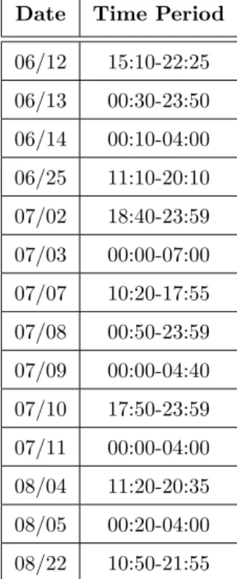
The date/time associated with each of the weather files given to us by Lincoln Laboratories is in UTC format, so we will use this convention throughout this thesis. To convert UTC to local time during the summer months, we subtract 5 from the UTC hour unit. The weather files consist of 14 days in June, July, and August 2008 in which weather, at some point, impacted the ORD terminal area. However, in this thesis, we specifically focus on time periods within these days in which severe convective weather penetrations took place in the ORD terminal area. Thus, we examine periods in which severe convective weather was present long enough to affect air traffic flows in a negative manner. These specific periods are outlined in Table 2.2.

Although there may be multi-hour gaps between penetrations within these periods, the table only includes one time period per day. Nonetheless, large time periods that last almost a full day indicate that weather impacted the ORD airspace consistently for a significant

Date Time Period 06/12 15:10-22:25 06/13 00:30-23:50 06/14 00:10-04:00 06/25 11:10-20:10 07/02 18:40-23:59 07/03 00:00-07:00 07/07 10:20-17:55 07/08 00:50-23:59 07/09 00:00-04:40 07/10 17:50-23:59 07/11 00:00-04:00 08/04 11:20-20:35 08/05 00:20-04:00 08/22 10:50-21:55

Table 2.2: List of severe convective weather penetration periods within the ORD terminal area during summer 2008.

amount of time.

2.2

ETMS Database

The Enhanced Traffic Management System (ETMS) was created by the FAA in order to monitor and react to traffic congestion in the United States using real-time trajectory data [1]. Air traffic controllers can leverage this data to direct aircraft flow and make decisions regarding Ground Delay Programs (GDP) and Ground Stop Programs (GS) [1].

The ETMS comprises a network of “hubsites” that transmit/receive trajectory data to/from several remotes sites throughout the United States using the Aircraft Situation Dis-play to Industry (ASDI) feed [1]. Trajectory data is automatically generated by transponders on aircraft and sent as real-time messages to the ASDI feed. In 2008, many aircraft, espe-cially general aviation aircraft, were not outfitted with transponders [14], so some flights

may be missing from the database. We have no way of identifying this missing flights. The Volpe National Transportation Center provided us with all ETMS data from 2008; this data consists of two main tables. The first table provides basic information about each flight such as arrival and departure airport, scheduled departure time, scheduled arrival time, actual arrival time, and aircraft type. ETMS also assigns a unique flight key to each flight so that flight information and trajectory information are linked. Several flights in the database have blank (NULL) fields, but these flights typically do not take place during the case periods.

The second table contains positional data for each flight at numerous points throughout the flight. This data includes transponder message time, latitude, and longitude. This table also includes a “smoothed” altitude that is derived using a moving average as well as an average speed that is derived from position and time data. Messages are sent from flight transponders approximately once a minute during the enroute portion of the flight and approximately once every 15-20 seconds during the ascent/descent portions of the flight. 2.2.1 Verifying ETMS Trajectory Data for Model Dataset

Like any large dataset, ETMS contains several data errors that required “cleansing” prior to analysis. Most of these errors were present in the trajectory data. One common error is the presence of gaps in trajectories because flight transponders may not transmit their position for long periods of time. Luckily, the majority of these gaps take place during the enroute portion of the flight, whereas we are concerned with trajectory gaps within the terminal area. When a flight is in its ascent or descent phase, it typically transmits its position every 15-20 seconds, if not more often. However, there are a handful of flights that have gaps much larger than 15-20 seconds. We chose to exclude flights from our model dataset that had a trajectory gap of greater than two minutes. Since the ascent/descent phases of flight last only 15-20 minutes, a gap larger than two minutes would represent a significant portion of

our observation period, during which a weather penetration may be missed. Additionally, our weather files represent 2.5 minute time periods, so gaps longer than this would skip over an entire weather file.

Another common error that occurs within approximately 30% of flight trajectories in the database is the presence of unreasonable altitude entries. For instance, consider a departure that is listed at an altitude of 2,500 feet at message two, 36,000 feet at message three, and then 4,200 feet at message four. It is apparent that there is an error in the altitude entry for message three. We corrected faulty altitude entries in different ways depending on their corresponding message number and whether they occurred within a departure vs. arrival trajectory.

All departures in the dataset record an initial altitude of zero. However, it is obvious that the initial transponder message did not take place at zero altitude because the initial position is some kilometers away from the runway or the altitude jump from the first to second transponder message is unreasonably large. Thus, we extrapolate the actual initial altitude using equations 2.1-2.3.

t1new = D1÷ δ t2− 0 (2.1) t2new = t1new+ t2 (2.2) a1new = a2 t2new ∗ t1new (2.3) where

D1 = distance from takeoff to first message

δ = distance from takeoff to first message t1new = time between takeoff and first message

t2 = original time spent in the air from takeoff to second message

t2new = new extrapolated time spent in the air from takeoff to second message

a1new = new extrapolated altitude at first message

a2 = original altitude value at second message

From these equations, we can also extrapolate an estimate for the actual takeoff time of the flight, which will be useful in the predictive models. The takeoff runway for each flight is assigned based on distance from each runway and the heading of the plane at the first message entry.

Moving on with unreasonable altitude entries with arrival trajectories, if the faulty entry took place at the first message entry within the terminal area, we would set the altitude value to the next altitude entry plus 300 feet. This ensures the trajectory will maintain a relatively smooth descent. On the other hand, if the faulty entry took place at the last message entry of an arrival trajectory within the terminal area, we would set the altitude value to the previous altitude value minus 300 feet. Similarly, for altitude misprints at the last message entry of a departure trajectory within the terminal area, we set the altitude to the previous altitude entry plus 300 feet to ensure smooth ascent. Finally, if the faulty altitude entry took place anywhere else in the trajectory, we set the new altitude to the

average of the altitude entries surrounding it. For example, if the altitude misprint took place at the 4th message, we set its value to the average of the altitudes at the 3rd and 5th message entry.

The initial and final positions of flights is also an area of concern within the data. On the departures side, as discussed above, the initial latitude/longitude of flights indicates a non-trivial distance away from ORD. Thus, the initial transponder message does not reflect the flight’s initial position at takeoff but rather some position later within the takeoff phase. Consequently, we limited the model dataset to departures with an initial position less than 10 km from the published latitude/longitude coordinates of ORD. Since the largest distance between takeoff runway and airport terminal at ORD is 3.25 km, any flight with initial position larger than 10 km has most likely been in flight for a couple minutes, representing a large gap in trajectory that we want to avoid. Moreover, it is very difficult to assign takeoff runways to flights with initial positions greater than 10 km from ORD.

Similar to departures, the final latitude/longitude of arrivals sometimes indicates a rela-tively large distance away from the published latitude/longitude coordinates of ORD. Con-sequently, we limited the model dataset to arrival trajectories with a final position less than 10 km from ORD. Beyond this distance, it was very difficult to assign landing runways, and a large portion of the flight would be left out of examination. Furthermore, the arrival trajectories often contain multiple message entries at the same altitude at the end of the trajectory. For our analysis, particularly when assigning landing runways, we assumed that the first of these message entries at the same altitude was the actual point of touchdown.

Overall, we removed approximately 5% of the flights, including both departures and arrivals, from the original model datasets due to the data errors discussed above.

2.3

ASPM Database

The Aviation System Performance Metrics (ASPM) is a FAA-built database of the National Airspace System providing airport and individual flight data for 77 airports and 22 carriers in the US [2]. This thesis accessed ASPM’s online “Efficiency Reports” to extract impor-tant airport data. The reports provide such useful information (in local time in 15-minute intervals) as runway configuration, wind speed, wind direction, visibility, and ceiling. Some of these metrics were used in preliminary models but had very weak predictive power. The metrics are accurate only within a 10 km radius of ORD rather than across the entire ter-minal area we defined. Nonetheless, the runway configuration data enabled verification of runway assignment algorithms used in the models and aided in the case studies presented in Chapter 6 by outlining airport operations in convective weather scenarios.

3

Feature Identification

When we discuss “features” in this thesis, we are referring to the independent variables in our predictive models. Our models utilize three different types of features: weather-based, in-flight behavior, and behavior of other flights in the terminal area. The following sections will discuss these three feature types in detail while presenting the different model features that fall within these groups. To make sense of these different model features, we must first discuss the three separate models examined in our research and their dynamic nature.

3.1

Three Separate Models

We first separated models by arrivals vs. departures because their behavior is inherently different in the terminal area, especially close to the airport. From a top-level perspective, the difference between them is clear: departures ascend while arrivals descend. However, the differences in their behavior can be characterized more granularly. When departures take

off, their horizontal and vertical movement is much less constrained than that of arrivals descending, making it easier to deviate around weather cells. Upon takeoff, departures are able to turn in a wide variety of directions right away, whereas arrivals on approach must follow specific landing patterns based on their assigned runway and the current wind direc-tion. Farther out from approach, arrivals are assigned to cornerposts and their corresponding streams by air traffic controllers.

In addition, there is pressure to get arrivals on the ground in a severe convective weather scenario. The situation at Chicago O’Hare adds to this pressure because diversion to its alternate airport, Midway (MDW), does not significantly improve weather conditions due to their very close proximity of less than 25 miles. Consequently, flights whose assigned runway is covered by severe convective weather may have no other option but to penetrate, as ATC rarely allows for runway reassignment. To pilots and airlines alike, this is a better option than continuing to fly around the terminal area burning fuel and subjecting the plane to further weather encounters, especially if storm cells are widespread throughout the terminal area. In contrast, on the departures side, ATC can slow or even halt departure operations altogether when severe weather is present because they are already on the ground.

We then separated the arrivals model into two separate models: one for the portion of the trajectory far from ORD and one for the portion of the trajectory close to ORD. The “close” model examines the trajectory starting 50 km out from O’Hare. We made this second model split because arrivals behave much differently within this 50 km radius from the airport. Within this boundary, arrivals are setting up their approach for landing. Based on a flight’s assigned runway, the direction it is coming from, and current wind conditions, a flight may actually have to fly past the airport in order to obtain the proper approach direction. Thus, within the 50 km radius, an arriving flight’s distance from the airport may fluctuate, making it harder to bin messages based on distance from the airport. We will discuss why this presents a problem for our original model design in the next section.

In total, we now have three separate models: one for departure trajectories, one for arrival trajectories outside 50 km from the airport, and one for arrival trajectories within 50 km from the airport. We will refer to these three models as “Model 1”, “Model 2”, and “Model 3” respectively in this thesis. Furthermore, although these three models will use many of the same features, there are some features that are unique to a particular model. We will discuss the assignment of features to models in the following sections.

3.2

Dynamic Nature of Models

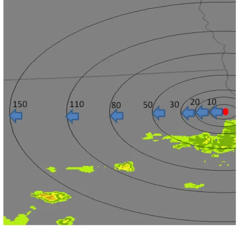
One main distinction between our models and Lin’s models is their dynamic nature, mean-ing that predictions are updated based on updated feature values at multiple checkpoints throughout a flight’s trajectory within the terminal area. The checkpoint intervals for Model 1 and Model 2 are defined based on distance from the airport and become larger as you move farther away from the airport. Figure 3.1 shows the Model 1 checkpoint intervals.

The red dot in Figure 3.1 represents the airport. The concentric half-circles represent the checkpoint boundaries. Moving outwards, penetration predictions are made at the checkpoint for the portion of the flight that takes place between the checkpoint and the next half-circle. For instance, suppose a departing flight is currently 80 km from the airport. The prediction for whether or not the flight will penetrate severe convective weather between 80 km and the next checkpoint boundary (110 km) will be made at the 80 km checkpoint. The feature values used for this prediction are calculated based on information obtained up to the current point in the flight. The final prediction in this scenario would take place at the 110 km checkpoint boundary because it is the beginning point of the last interval in the terminal area.

The Model 1 and 2 checkpoint intervals were constructed based on the distribution of penetration entries by distance from ORD, shown in Figure 3.2.

Figure 3.2: Distribution of Penetrations by Distance from ORD

Arrival and departure penetrations follow a similar distribution, with most penetrations taking place within 30 km of ORD. Some penetrations take place between 40 and 100 km

from ORD, and then very few take place beyond this point1_{. Our prediction intervals reflect}

this distribution, with more frequent, shorter intervals closer to the airport and less frequent, larger intervals farther from ORD. The intervals become larger as the flight gets farther away from the airport because behavior becomes more consistent at these farther distances and because time between transponder messages is longer2. Specifically, for Model 1, predictions are made for the following intervals: between takeoff and 10 km, between 10 km and 20 km, between 20 km and 30 km, between 30 km and 50 km, between 50 km and 80 km, between 80 km and 110 km, and between 110 km and 150 km. Model 2 predictions work almost identically except that the predictions are made in the opposite direction moving towards the airport, starting at 180 km out and ending with a prediction between 80 and 50 km.

Model 3’s prediction intervals are based on time spent within 50 km of the airport instead of distance from the airport. Model 3 is designed this way because arrivals’ distance from the airport often fluctuates within 50 km due to varying approach paths such as “trombon-ing”, holding patterns, and other maneuvers that make it impossible to create consistent checkpoint boundaries. For Model 3, predictions are made every 2.5 minutes of flight. Thus, when an arrival first enters the 50 km radius, the model predicts whether it will penetrate severe convective weather within the next 2.5 minutes of flight. This process continues until the flight lands. This time-based prediction approach is hypothetically much more difficult than the distance-based prediction approach utilized in Model 1 and 2 for two main reasons: 1) a lot can happen in 2.5 minutes of flight and 2) flight behavior is already more uncertain close to the airport. Flights that spend more than 25 minutes within the 50 km radius before landing were excluded from the model dataset. Such cases were very rare and exhibited flight behavior that often did not make sense, suggesting errors in the recorded trajectory.

In reality, the structure of our models may be better described as semi-dynamic than dynamic because we group information from multiple trajectory message entries into a finite

1_{The plot shows that there are no departure penetrations past 150 km because that is the boundary for}

our terminal area with respect to departure flights. This boundary is 180 km for arriving flights.

number of bins based on checkpoint boundaries. A purely dynamic model would, in contrast, make a prediction at each message time along the trajectory. We chose to use semi-dynamic models rather than purely dynamic models because semi-dynamic models are better able to capture overall flight behavior and traffic flows during weather impacts. Additionally, purely dynamic models would require predictions every 15-20 seconds during ascent/descent. This would necessitate not only magnitudes more computing power but could also result in “information overload” for air traffic controllers who use our prediction tool.

3.3

Weather-Based Features

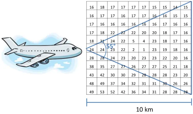
This group of features exploits the weather data discussed in Chapter 2 to characterize the current weather scenario that a flight is experiencing. For instance, if convective weather is on top of ORD and its surrounding area out to 10 km, one would assume that many flights will penetrate upon takeoff or landing. However, our model’s weather-based features do not aim to characterize the weather scenario within the ORD terminal area as a whole, but rather focus on weather in relation to a flight’s projected trajectory. This fundamental difference from Lin’s weather-based features makes sense considering the dynamic nature of our models and our interest in specific segments of a flight’s trajectory during ascent/descent. An example of the projection from which we calculate our weather-based features is shown in Figure 3.3.

The matrix shown within the projection represents the VIL values corresponding to individual pixels within the projection. These VIL pixel values are vertical columns that extend infinitely into the atmosphere. All of the pixels that are within the triangle formed by the blue lines, including those that intersected by the triangle’s edges, are considered part of the trajectory projection. The length and swath width of the projection may vary based on the current prediction checkpoint boundary. Values of 10 km and 65 degrees are typical of projections for smaller intervals closer to the airport. The length of projections

Figure 3.3: Projected flight trajectory looking 10 km out with swath width of 55 degrees. Angles and distances are not exactly to scale.

is usually equal to the interval distance, and the swath width is adjusted to account for potential horizontal movement of the flight within an interval.

The weather-based features are calculated from the VIL values associated with the group of pixels within the projection. Echo top values, however, are not considered in our weather-based features. If an echo top value exists for a pixel within the terminal area, which requires a VIL level≥3, most observed flights will be below this echo top because they are below cruising altitudes. Thus, thorough examination and manipulation of these values would be redundant. Nevertheless, these echo top values still serve as limiting criteria for penetration classification.

Furthermore, the weather-based features can be divided into three distinct groups: one group measuring the severity of weather within the projection, one group measuring the movement of weather within the projection, and a third group measuring the spatial po-sitioning of weather cells within the current prediction interval. We describe the features within each group in the sections below. Every one of these features is included in Models

1, 2, and 3.

3.3.1 Measuring Severity of Weather

This subset of weather-based features aims to capture the strength of the storm cells, if present, within the trajectory projection. Intuitively, if a flight’s projection contains a large amount of strong storm cells, there is a good chance that the flight will penetrate in that interval, unless it deviates around the weather or the weather moves. We use two different features to measure the severity of weather within a flight’s projection, with both features measuring the proportion of cells within the projection that have VIL level greater than or equal to 3 (VIL value≥133). The features differ in the set of VIL pixels they examine: the first feature (“BadWeatherPercentageBefore”) evaluates the pixels within the projection from the prior weather data time period, whereas the second feature (“BadWeatherPercent-ageNow”) evaluates the pixels from the current weather data time period. Our weather data files are broken up into 2.5 minute periods, so if the current time is 10:30:00 UTC, then “BadWeatherPercentageBefore” would look at pixel data from the 10:27:30 weather file, and “BadWeatherPercentageNow” would like at pixel data from the 10:30:00 weather file. An example calculation, independent of time, of these features for a 15-pixel rectangular projection can be seen in Figure 3.4, with severe VIL values in red.

Figure 3.4: Calculation of weather-based feature that measures severity.

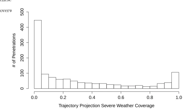
around 15% and 30%, compared to a value of 0% and 2% for non-penetrations. However, Figure 3.5 reveals that the large majority of penetrations takes place when the values for these features are below 10%. Thus, weather coverage does not have to be particularly overwhelming to give pilots trouble.

Trajectory Projection Severe Weather Coverage

# of P enetr ations 0.0 0.2 0.4 0.6 0.8 1.0 0 100 200 300 400 500

Figure 3.5: Distribution of penetration entries by severe weather coverage within the trajec-tory projection.

3.3.2 Measuring Movement of Weather

This subset of weather-based features aims to capture the movement of weather within the projection by examining how weather conditions change from one time period to the next. The first feature (“PercentBadCellsDiffVIL”) calculates the difference, between time periods, in the proportion of pixels within the projection that have VIL level ≥ 3. The second feature (“SeverityDiffVIL”) calculates the difference in overall severity score of the projection between time periods. To calculate this overall severity score, each pixel within the projection is first assigned a VIL level based on its raw VIL value using Figure 2.1. The overall severity score is simply the sum of the VIL levels for all of the pixels within the projection. The third feature (“PercentWorseningVIL”) calculates the proportion of pixels within the projection that increase in VIL value between time periods.

The next two features are very similar in the way in which they are calculated, but their output describes the weather situation within the projection in very different manners. The features calculate the sum of the difference in VIL value between corresponding projection pixels between time periods. The distinction between the features is that one (“CellDiffVIL”) calculates the raw pixel-to-pixel difference, including sign, whereas the other (“CellDiffVI-LAbs”) calculates the absolute difference before summing up all of the pixel differences. Figure 3.6 displays the calculation processes for these two features using the same initial set of pixel values extracted from the middle of the projection region in Figure 3.3.

Figure 3.6: Calculation of weather-based features that measure movement.

To obtain the final pixel value differences on the far right, we subtract the Time 1 pixel values from the Time 2 pixel values. In this example, the VIL pixel values stay the same between Time 1 and Time 2 but switch positions within the square projection. Thus, the sum of the pixel values is 12 for both time periods. However, the final feature value, or the sum of the differences, is 0 for the first feature and 12 for the second feature. Hence the first feature captures the fact that the values and their sum within the projection have not changed, whereas the second feature recognizes the movement of the values within the projec-tion. Consequently, we hypothesize that the absolute difference feature (“CellDiffVILAbs”)

captures weather movement better than the raw difference feature (“CellDiffVIL”). How-ever, it is worth noting that the raw difference feature describes how the strength of weather within the projection changes between time periods, augmenting the subset described in the previous section.

The final value used for each weather movement feature within the predictive models is the average of the feature values for two time period differences before the current time in order to best capture the situation at hand while only exploiting information that is already known at the time of prediction. For instance, if the current time is 10:30:00 UTC, we would average the feature values corresponding to the 10:22:30 and 10:25:00 weather file pairing as well as the feature values corresponding to the 10:25:00 and 10:27:30 weather file pairing. 3.3.3 Spatial Positioning of Weather

This last subset of weather-based features aims to capture the spatial positioning of weather cells ahead of the flight being observed. These features do not constrain the trajectory projection with a swath width. Instead they consider all pixels in front of the plane within the specified interval distance. The first feature (“flankcount”) counts the number of pixels in this widespread projection that have VIL level ≥ 3. The count is weighted based on the distance of the pixel within the projection from the plane’s current position, with weight decreasing incrementally as distance from the plane increases. For example, a severe weather pixel that is located 10 km from the plane’s current position is worth more than a pixel that is located 20 km from the plane’s current position. This weighting scheme makes sense because storm cells closer to the plane’s current position provide more immediate danger and are less likely to migrate out of the projection before the plane encounters them.

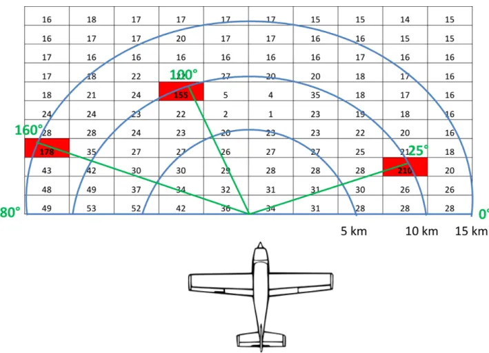
The second feature (“FlankingValue”) is a bit more complicated. It sets the nose of the plane as the common center of several concentric half circles whose radius depends on the distance of a severe weather pixel from the center. We then calculate the degree value

(between 0 and 180) of each severe weather pixel based on its position on one of the concentric half circles. The feature value is the standard deviation of the degree values of the storm cells. By using the standard deviation, we capture the span of the storm cells across the plane’s nose. If there are no storm cells within the interval ahead of the flight, then the feature value is 0. A large standard deviation hypothetically reflects that there are storm cells all across the plane’s direction of movement, making it harder to deviate around the storm cells or find pockets without weather. Figure 3.7 displays how we identify the degree values for this second flanking feature.

Figure 3.7: Example of flanking metric calculations with the number of red cells representing “flankcount” and the standard deviation of the degree values representing “FlankingValue”. The red pixels contain severe VIL values, so we include them in our feature calculations. The radii of the concentric half circles is based on the severe weather pixel’s distance from the

current flight position. The radii values matter more for the “flankcount” weighting scheme than for the “FlankingValue” feature. In this example, the “FlankingValue” feature value would be the standard deviation between 160, 100, and 25: 67.64. This value represents a fairly large spread of severe weather cells across the plane’s nose. However, it is apparent that this feature does not capture whether there is a concentration of severe weather cells in one particular region of the relaxed projection. Possible improvement of this feature will be discussed in the “Future Work” section in Chapter 6.

Since “flankcount” values differ based on the size of the trajectory projection, we will not present their summary statistics. Nonetheless, it is apparent that penetrations consistently encounter trajectory projections with a much larger “flankcount” than non-penetrations.

With regards to “FlankingValue”, the median and average values for these features given a penetration are respectively around 18 and 21, compared to a value of 0 and 2 for non-penetrations. Thus, the typical trajectory projection of penetrations not only contains sig-nificantly more severe weather pixels, but these pixels are more spread out across the nose of the plane. Nonetheless, it is worth noting that the maximum “FlankingValue” for pene-trations was approximately 40, so the severe weather pixels are still relatively concentrated within the projection.

3.4

In-Flight Features

The next set of features we will discuss deals with the behavior of the flight of interest within the terminal area and how this behavior may be correlated with severe convective weather penetration. These in-flight features are broken down into three subsections below.

In addition to features that deal with the behavior of the flight of interest, our models consider standard characteristics about the flight, for instance, whether it is an international flight (“intl”) and/or a cargo (“car”) flight. We also note whether the flight’s ascent/descent sequence takes place during darkness (“night”) between the hours of 21:00:00 and 06:00:00

local time.

Although delays hypothetically fall under in-flight features, we did not include them in our arrivals models based on their weak predictive power in Lin’s models, which exclusively examined arrivals. Exclusion of delay features makes sense on the departures side as well because most departures during weather impacts are delayed. The fact that only a small percentage of the total number of departures during these weather-impacted periods are penetrating supports this exclusion.

3.4.1 Time Spent Within Terminal Area

The first subset of in-flight features keeps track of the time that a flight has spent in the terminal area up to the current prediction checkpoint. Models 1 and 2 consider total time spent in the terminal area (“TimeinTerm”), from the time departures take off or arrivals enter the terminal area. Model 3 considers this metric as well as the time spent within 50 km (“TimeWithin50km”) from the airport, reflecting the different approach maneuvers performed by arrivals prior to landing. Rare flights that spent excessive amounts of time in the terminal area, specifically 25 minutes within 50 km or 50 minutes overall, were excluded from the model datasets due to their unexplained behavior.

One may assume that longer flight times within the terminal area would be less correlated with weather penetration since they might reflect deviation to avoid weather. However, our case studies indicate that typically pilots are unable to deviate around weather completely because blockage is too extensive. This is especially the case when weather is close to the airport and range of motion is limited. Hence longer flight times within the terminal area do not always translate to pilot deviation.

Overall, we included these features in our models due to their strong performance in Lin’s models and the notion that longer flying times translate to more exposure to weather.

3.4.2 Flight Behavior Within Terminal Area

The next subset of in-flight features aims to capture certain behavioral tendencies of flights in their ascent/descent phase. The first feature within this subset (“LevelOffORDecreasing”) applies to all three models, observing whether or not flights are leveling off within their trajectory. Although this behavior is systematic within the terminal area based on stan-dardized routes, we found that flights frequently penetrate while leveling off. This was even the case for departures, which are not commonly restricted to step-like paths like arrivals. Furthermore, flights on bad-weather days tend to level off more often than flights on days without weather. Figures 3.8-3.10 exhibit this behavior for departure flights, with leveling off maneuvers typically occurring at 5000 ft altitude beginning 15 km from the airport. Each individual trajectory curve within the plots represents a different flight.

Figure 3.8: Plot of Altitude vs. Distance from Takeoff for departure trajectories on July 2nd that penetrated severe convective weather.

The July 2nd plots (Figures 3.8 and 3.9) exhibit several cases of leveling off behavior, whereas the occurrences of level offs in the June 10th plot are much fewer. Furthermore,

Figure 3.9: Plot of Altitude vs. Distance from Takeoff for departure trajectories on July 2nd that took place during a weather impact but did not penetrate.

Figure 3.10: Plot of Altitude vs. Distance from Takeoff for departure trajectories on June 10th with no weather impact.