HAL Id: hal-00304657
https://hal.archives-ouvertes.fr/hal-00304657
Submitted on 1 Jan 2002HAL is a multi-disciplinary open access archive for the deposit and dissemination of sci-entific research documents, whether they are pub-lished or not. The documents may come from teaching and research institutions in France or abroad, or from public or private research centers.
L’archive ouverte pluridisciplinaire HAL, est destinée au dépôt et à la diffusion de documents scientifiques de niveau recherche, publiés ou non, émanant des établissements d’enseignement et de recherche français ou étrangers, des laboratoires publics ou privés.
C. de Michele, R. Rosso
To cite this version:
C. de Michele, R. Rosso. A multi-level approach to flood frequency regionalisation. Hydrology and Earth System Sciences Discussions, European Geosciences Union, 2002, 6 (2), pp.185-194. �hal-00304657�
A multi-level approach to flood frequency regionalisation Hydrology and Earth System Sciences, 6(2), 185–194 (2002) © EGS
A multi-level approach to flood frequency regionalisation
Carlo De Michele and Renzo Rosso
DIIAR, Politecnico di Milano, Piazza Leonardo da Vinci, 32, I-20133 Milano MI, Italy Email for corresponding author: [email protected]
Abstract
A multi-level approach to flood frequency regionalisation is given. Based on observed flood data, it combines physical and statistical criteria to cluster homogeneous groups in a geographical area. Seasonality analysis helps identify catchments with a common flood generation mechanism. Scale invariance of annual maximum flood, as parameterised by basin area, is used to check the regional homogeneity of flood peaks. Homogeneity tests are used to assess the statistical robustness of the regions. The approach is based on the appropriate use of the index flood method (Dalrymple, 1960) in regions with complex climate and topography controls. An application to north-western Italy is presented.
Keywords: homogeneity, multi-level approach, regionalisation, seasonality, scale invariance, similarity, tests
Introduction
The identification of homogeneity at regional scale is a basic step in the inference of the estimation of flood probabilities. This operation is traditionally carried out using statistical methods of the parametric and non-parametric type (e.g. Natural Environmental Research Council, 1975; Tasker, 1982; Potter, 1987; National Research Council, 1988, among others) with large uncertainties and a certain degree of subjectiveness mainly due to the lack of a rigorous physical basis. This deficiency has recently led to the introduction of the concept of scale invariance of annual maximum flood to identify homogeneous regions in flood frequency regionalisation (Gupta and Waymire, 1990; Gupta and Dawdy, 1994; Gupta et al., 1994; De Michele and Rosso, 1995; Robinson and Sivapalan, 1997a). Thus, the T-year flood quantile, QT, is proportional to a power law of the drainage area, A, QT(A)
∝
Am, with a scaling exponent, m,characteristic for all the river basins located in the homogeneous region. Yet the small variability of m, between 0.4 and 0.9 (see e.g. De Michele and Rosso, 1995) often does not allow a homogeneous region to be delimited and the grouping of the river basins is carried out empirically. Physical criteria have to drive this important step of the regionalisation procedure. The analysis of the mechanisms of flood production can provide useful information on the
clustering of river basins. Robinson and Sivapalan (1997b) investigated the influence of the different time scales (storm duration, catchment response time, inter-arrival time) on the hydrological regimes and the implications on the flood frequency analysis. Institute of Hydrology (1999) used the concept of similarity distance measure to judge the similarity of two catchments and identify the pooling of groups of catchments in Great Britain. Burn (1997) introduced seasonality measures as catchment similarity indices for the regional flood frequency analysis. Piock-Ellena et al. (1999) and Merz et al. (1999) considered some seasonality indices (Pardé index, Pardé (1947) and Burn’s vector, Burn (1997)) of runoff and precipitation to infer the main flood-producing mechanisms in Austria.
In this paper, a multi-level approach to flood frequency regionalisation is presented based on physical and statistical criteria. In particular, seasonality indices are used to cluster basins with the same flood production mechanism, simple scale invariance is used to verify the homogeneity of identified regions, and homogeneity tests to assess the statistical robustness of the clustered regions. The following section deals with the seasonality indices used, i.e. Pardé index (Pardé, 1947) and Burn’s vector (Burn, 1997). In the next section, the scaling invariance of annual maximum flood and regional homogeneity are discussed. Finally, the
multi-level approach is outlined, and its application to flood regionalisation in north-western Italy is reported and discussed.
Hydrological similarities: seasonality
indices
Robinson and Sivapalan (1997b) identified some temporal scales to characterise the hydrological flood regimes. They found that the combined effects of within-storm patterns, multiple storms, and seasonality have an important control on the observed scaling behaviour in empirical flood frequency curves. The effect of seasonality on the determination of hydrological similarities is investigated here. Following Piock-Ellena et al. (1999) and Merz et
al. (1999), one can take into account two seasonality indices:
the Burn’s vector (Burn, 1997) and the Pardé coefficient (Pardé, 1947). The first index characterises the seasonality on the extreme events, the second one considers the seasonality on monthly variables.
BURN’S VECTOR
This index was introduced by Burn (1997) to investigate the seasonality of annual maximum floods. It is a vector that represents the variability of the date of occurrence of a flood event; in particular, its direction is the mean date of occurrence of annual maximum flood and the modulus is the variability around the mean value. Considering the date of occurrence of the annual maximum flood event as a Julian date, where January 1 is the 1st day and December 31 is the
365th day, and converting it into an angle in radians, one has
( ) π = θi JulianDatei 3652 .
Thus, the date of annual maximum flood event can be interpreted as a vector with a unit magnitude and direction θi. The mean direction of an n-events sample is given as
= θ − x y tan1 , (1)
where θ is in radians and
∑
= θ = n i i cos n x 1 1 and
∑
= θ = n i i sin n y 1 1 .The variability around the mean value is obtained by calculating the modulus of the average vector with:
2
2 y
x
r= + . (2)
The couple ( θ , r) defines the Burn’s vector. θ is expected to be related to other important catchment characteristics
such as size, geographical location and dominating supply factor (glacier ablation, snowmelt, rainfall). r provides a dimensionless measure of the spread of the dates of occurrence. It assumes values between 0 and 1. For r → 0 there is no single dominant flood season and the time of occurrence of annual maximum flood is distributed around year; for r = 1 the annual maximum flood occurs on the same day. Thus larger values indicate greater regularity in the time of occurrence. Low values could be explained with the existence of different flood mechanisms that play an important role in the generation of annual maximum flood, such as snowmelt and rainfall precipitation.
PARDÉ COEFFICIENT
The Pardé coefficient (Pardé, 1947) considers the seasonality of maximum mean monthly flow. Let Qij denote the observed value for the month i in the year j. For each month, it is defined by the index
∑
∑
= = = n j i ij ij i Q Q n Pk 1 12 1 12 . (3)where n is the number of years. The Pardé coefficient is given by the couple
( )
(
imax,Pk=Max Pki)
, (4)where imax is the month in which Pk occurred. The sum of
Pki is always equal to 12. Pki equal to 1 for all i corresponds to a constant value of monthly flow in the year. If all maximum mean monthly flows occur in month imax, then
Pki = 0, for i ≠ imax, and Pk = Pkimax = 12. Thus Pk varies in the range 1 to 12. In the same way as Burn’s index, the Pardé coefficient can be represented by a vector with modulus proportional to Pk and direction proportional to imax.
Regional homogeneity and scale
invariance of annual maximum flood
The definition of a homogeneous region is a basic requirement in flood frequency regionalisation according to the index flood method. Following Gupta et al. (1994) and Robinson and Sivapalan (1997a), a group of basins is homogeneous if the annual maximum flood scales is a function of its drainage area. Let Q(A) be the annual maximum flood in a river as parameterised by its drainage area A. Let Ai and Aj be the areas of two basins in a particular region Ω. It is homogeneous if( )
[
Q Ai]
F[
g(
Ai,Aj) ( )
QAj]
A multi-level approach to flood frequency regionalisation
where g(.) is a random or not random function and F(.) is the cumulative distribution function. Note that Eqn. (5) represents also the spatial scale invariance of Q(A) with drainage area.
Lamperti (1962) provided the analytical form of the scale function, g(Ai, Aj) = (Ai/Aj)m, where the exponent m is a
fundamental parameter representing the aggregation or the disaggregation of the underlying physical process from one scale to another. Inverting Eqn. (5) and taking Ai = A and
Aj=1, the flood quantiles parameterised by area scale is
( )
( )
m TT A Q A
Q = 1 . (6)
The scaling exponent m is an important function of the complex interactions between climate and surface hydrology producing flood flows; it allows the scaling of a specified flood quantile for any basin from that for a basin with unit area. Note that the ratio QT1
( )
A /QT2( )
A between two flood quantiles with return periods of T1 and T2, respectively, is independent of area.Equation (6) defines the property of statistical simple scaling in a strict sense according to Gupta and Waymire (1990). In the same way, the k-th order statistical moment of flood flows, with respect to the origin, scale with the drainage area as
( )
[
Qk A]
AkmE[ ]
Qk( )
1E = , k = 1, 2, ... (7)
where E[.] denotes the expectation operator. Gupta and Waymire (1990) used Eqn. (7) to define statistical simple scaling in a wide sense, because Eqn. (7) is derived from Eqn. (6), but the circumstance that Eqn. (7) holds does not prove that Eqn. (6) holds automatically. From Eqn. (7) the dimensionless coefficients of variation, skewness and kurtosis are independent of drainage area.
Combining Eqn. (6) with Eqn. (7) for k = 1, Gupta et
al. (1994) showed that the T-year flood quantile normalised
by its mean is the same for all subcatchments included in the homogeneous region. This is the principal assumption of the index flood method for regional flood frequency analysis. Because of the complexity of the underlying physical processes, and insufficient sampling of random processes describing extreme events, it is rather difficult to verify Eqn. (6) by investigating the scaling exponent of QT with varying basin area A. Therefore, wide sense simple scaling as represented by Eqn. (7) can be accepted as an indication of self-similar flood probabilities in a river system or in a geographical region.
Questions about the existence of statistical moments of extreme flood probabilities were raised by Turcotte and Greene (1993) in the analysis of ten annual maximum flood
series in the United States. Their fractal model accommodating the given data has vanishing moments for
k ≥ 2 for seven out of ten series. This also occurs when modelling the annual maximum flood series by the general extreme value distribution, GEV, for increasingly high negative values of its shape parameter. Therefore, the use of sampling statistical moments may contrast with the underlying flood frequency distribution and alternative methods must be used to assess simple scaling. Kumar et
al. (1994) approached scale invariance in geophysical
processes using the probability weighted moments (henceforth referred to as PWMs). Accordingly, wide sense simple scaling of flood probabilities occurs if
( )
[
Q A]
A k[ ]
Q( )
1 m k = β β , k = 0, 1, 2, ... (8) where( )
[
]
{
( )
[ ]
k}
Q k Q A =E Q A F β (9)is the k-th order PWM as parameterised by its area A, and
FQ is the cumulative distribution function of Q(A). The PWMs provide an efficient method for estimating extreme value distributions as shown by Greenwood et al. (1979) and Hosking (1986).
The concept of multiple scale invariance, or multifractal, was introduced to explain the variability of the exponent m in the power law (6), or in Eqn. (8), in which it varies with return period T, or with the order of statistical moment (Gupta and Waymire, 1990; Waymire and Gupta, 1991). If
n(k) is the value of the exponent in the scaling equation
between the k-th order statistical moment or PWMs and basin area, the convexity of n(k) with k implies multiscaling of the underlying process, as opposed to linearity characterising simple scaling or self-similarity of the process. Alternative methods to discriminate between simple and multiple scaling are reported by Schertzer and Lovejoy (1987) and Lovejoy and Schertzer (1990), among others. However, these methods can hardly be applied to relatively short samples as those provided by annual maximum flood series. Therefore, Eqn. (7) is used here to test the regional homogeneity of the clustered regions identified by seasonality analysis. In addition, the PWMs are also computed because of possible inconsistencies in the statistical moment approach due to non-existing high order moments of the parent probability distribution.
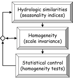
MULTI-LEVEL APPROACH
The multi-level approach to flood frequency regionalisation includes seasonality, scale invariance and appropriate statistical tests for homogeneity. This approach
Fig. 1. Schematic representation of the multi-level approach
Fig. 2. Study area Fig. 3. Pardé index for monthly precipitation uses seasonality indices to cluster catchments with the same
flood production mechanism, in other words, to capture hydrological similarities and thus to identify the potential homogeneous regions. It then considers the scale invariance of annual maximum flood, as parameterised by basin area, to check the regional homogeneity of clustered catchments. Finally, statistical homogeneity tests, L-moment ratio plots (Hosking and Wallis, 1993) and the Wiltshire test (Wiltshire, 1986) are used to assess the statistical robustness of the clustered regions. Figure 1 gives a schematic representation of the proposed methodology.
Case study
DESCRIPTION OF THE STUDY AREA
North-western Italy includes Lombardia, Piemonte, Valle d’Aosta, Liguria, and Emilia-Romagna regions (see Fig. 2). Climate is highly variable in the study area, through the
multifaceted controls by the atmospheric fluxes from the Mediterranean Sea, and the complex relief including the southern range of the western and central Alps and the northern Apennines range. In north-western Italy 344 gauging stations provide consistent records of monthly precipitation and annual maximum daily precipitation, with a mean length of sample of 35 years. In addition, there are 80 gauging stations providing consistent records of monthly stream flow and annual maximum flood with a mean length of sample of 28 years and with drainage areas ranging from about 10 to 2500 km2. Additional flood gauging station are
available for river sites with larger drainage areas but these data are not included in the present analysis because they are strongly influenced by the effects of river regulation and training works.
SEASONALITY ANALYSIS
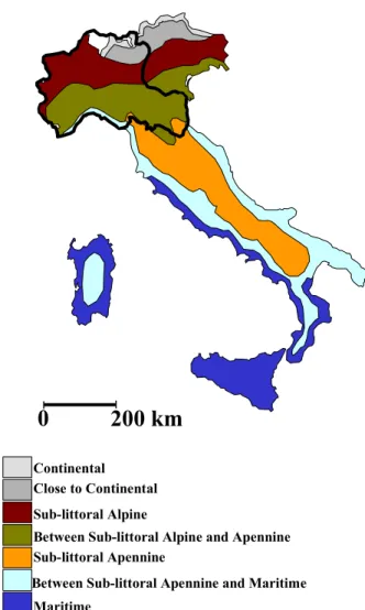
Seasonality of rainfall, floods and streamflow is investigated to understand the causes of flood production and thus the catchment similarities. To this aim we consider the Pardé index and the Burn’s vector. Figure 3 shows the Pardé index for the monthly precipitation. Clearly, there are two distinct regions. Both are rather uniformly distributed around the year and Pk is everywhere lower than 2.5. However, in Alpine catchments (upper part of the graph), the annual maximum monthly precipitation occurs from June (western basins) to September (eastern basins), while in the Apennines catchments (lower part of the graph), Pk occurs later, from November to January. This result is in agreement with the map of the season of the greatest monthly precipitation in Europe reported by Sumner (1988, p.341) and also with the spatial distribution of precipitation regimes in Italy as first introduced by Bandini (1931) and reported in Fig. 4. These regimes were determined by annual precipitation totals and by the distribution of monthly
3 4 5 6 7 8 x 10⁵ 4.80 4.85 4.90 4.95 5.00 5.05 5.10 5.15 5.20 5.25x 10 6 East UTM Nor th UT M . Oct July April . Jan 1 1 1 1 ↓ ← ↑ → Hydrologic similarities (seasonality indices) Homogeneity (scale invariance) Statistical control (homogeneity tests)
A multi-level approach to flood frequency regionalisation
precipitation within the year. Accordingly, these range between the continental and maritime regime in Italy. The first is characterised by a maximum of monthly precipitation in summer (July and August) and a minimum in winter (January and Febrary). Conversely, the second has a maximum of monthly precipitation in winter (between November and January) and a minimum in summer (July and August). Between these two there are five other intermediate precipitation regimes, namely close to
continental, littoral alpine, intermediate between sub-littoral alpine and sub-sub-littoral apennine, sub-sub-littoral apennine, and intermediate between sub-littoral apennine and maritime. All these regimes are characterised by two
maxima and two minima in the distribution of monthly precipitation. In particular, the sub-littoral alpine regime has the absolute maximum in autumn and a second one in spring (or vice versa) and the absolute minimum in winter. The intermediate between sub-littoral alpine and sub-littoral
apennine regime has the absolute maximum in autumn and
two minima of equal magnitude in summer and winter. The sub-littoral apennine regime is characterised by the absolute maximum in autumn and a minimum in summer. The close
to continental regime has intermediate characterisics
between the continental and sub-littoral alpine regimes. In a similar way, the intermediate between sub-littoral
apennine and maritime is a transitional regime between the
sub-littoral apennine and maritime regimes.
Comparing Figs. 3 and 4, note that the region of the Alpine catchments (upper part in Fig. 3) includes the following regimes: continental, close to continental, sub-littoral alpine and intermediate between sub-littoral alpine and apennine, all characterised by the maximum of monthly precipitation in the seasons summer–autumn in agreement with the results in Fig. 3. The region of Apennine catchments (lower part in Fig. 3) includes the intermediate between sub-littoral alpine
and apennine, sub-littoral apennine, the intermediate between sub-littoral apennine and maritime, and maritime
regimes, all characterised by the maximum of monthly precipitation in the period autumn-winter.
The same information presented in Fig. 3, but not as pronounced, is given by Burn’s vector for annual maximum daily precipitation, shown in Fig. 5. This is due to the greater variability of the quantity considered in the Burn’s vector. A more explanatory identification of clusters with different behaviour patterns can be obtained by analysing the seasonality indices for the monthly stream flows. Figure 6 shows the Pardé index for the maximum mean monthly stream flow. In Fig. 6, the region of Apennine catchments is divided into two with different behaviours. In the first one, Pk occurs from November to December and in the other from January to March. Conversely, in the region of Alpine catchments, Pk occurs from June to August.
Additional information is given by Burn’s vector of annual maximum flood (see Fig. 7). It distinguishes two Alpine clusters according to different values of θ. Burn’s vector
Fig. 5. Burn index for maximum annual daily rainfall
Fig. 4. Precipitation pattern in Italy and boundaries of the study area.
0
200 km
Continental Close to Continental Sub-littoral Alpine
Between Sub-littoral Alpine and Apennine Sub-littoral Apennine
Maritime
Between Sub-littoral Apennine and Maritime
3 4 5 6 7 8 x 10⁵ 4.80 4.85 4.90 4.95 5.00 5.05 5.10 5.15 5.20 5.25x 10 6 East UTM Nor th UT M . Oct July April . Jan 1 1 1 1 ↓ ← ↑ →
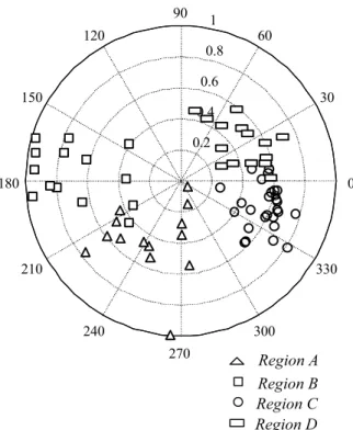
supports the discrimination of the two Apennines clusters. Figure 8 shows the polar representation of Burn’s index for the four identified regions (two Alpine and two Apennines clusters). It is important to note that the clustered groups occupy quite distinct sectors of the diagram. Thus the seasonality analysis identified four regions (two in the Alps and two in the Apennines) for north-western Italy, namely: z Region A or Central Alps and Prealps, that includes
Po sub-basins from Chiese to Sesia river basin, z Region B or Western Alps and Prealps from Dora Baltea
river to Rio Grana,
z Region C or North-Western Apennines and Thyrrhenian
basins that includes Ligurian basins with outlet to the
Thyrrhenian sea and Po sub-basins from Scrivia river basin to Taro river basin,
z Region D or North-Eastern Apennines from Parma to Panaro river basin (including Adriatic basins from Reno to Conca river basin).
The seasonality analysis of annual maximum flood identifies
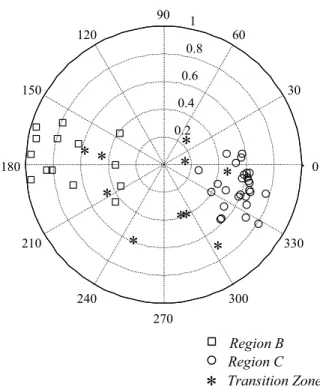
also a transition zone (the shaded area in Fig. 7). The transition zone (also referred to as TZ) is defined as one or more catchments, generally geographically located on the boundaries of the homogeneous regions that cannot be attributed effectively to any group, due to anomalous behaviour. Such anomalies could be ascribed to either local micro-climatic disturbances or superimposition of the different behaviours characterising the neighbouring regions. The transition zone identified corresponds to the Tanaro catchment. Some of its tributaries rise in the Alps, others in the Apennines. A gradual passage from the behavior of Region B to that one of Region C characterises this catchment. Figures 9 and 10 show the polar representation of the Burn’s vector for rainfall and flood of Region B, C and TZ, in which the anomalous behaviour of the transition zone is evident.
STATISTICAL SELF-SIMILARITY OF ANNUAL MAXIMUM FLOOD
Table 1 shows the estimated values of the scaling exponent of the k-th order statistical moment of the maximum annual flood with the relative standard errors, s.e., and the coefficient of determination R2 for the four regions
identified. Because of the short length of some data series, a maximum value of k = 4 is considered. Performing linear regressions on the observed data in the log E[Qk(A)] – log[A]
plane it is possible to estimate the scaling exponents of the Fig. 6. Pardé index for maximum mean monthly stream flow.
Fig. 7. Burn’s index for annual maximum flood.
Fig. 8. Polar representation of Burn’s index for annual maximum
flood for the homogeneous regions.
3 4 5 6 7 8 x 10⁵ 4.80 4.85 4.90 4.95 5.00 5.05 5.10 5.15 5.20 5.25x 10 6 East UTM Nort h UT M . Oct July April . Jan 1 1 1 1 ↓ ← ↑ → 3 4 5 6 7 8 x 10⁵ 4.80 4.85 4.90 4.95 5.00 5.05 5.10 5.15 5.20 5.25x 10 6 East UTM No rt h UT M
A
B
C
D
TZ
. Oct July April . Jan 1 1 1 1 ↓ ← ↑ → 0.2 0.4 0.6 0.8 1 30 210 60 240 90 270 120 300 150 330 180 0 Region A Region B Region C Region DA multi-level approach to flood frequency regionalisation
Fig. 9. Polar representation of Burn’s index for rainfall for region B,
region C and transition zone TZ.
Fig. 10. Polar representation of Burn’s index for annual maximum
flood for region B, region C and transition zone TZ.
statistical moments. From Table 1, the variability of the scaling exponents of the statistical moments is practically negligible for all the regions identified. The sample variability of the scaling exponent m with the order of the moment k is < 0.02 except for Region D where the difference [m(4)–m(1)] is 0.04; in all the cases the variability of the scaling exponent with the order of the moment, k, is included in a standard deviation. It is seen that the explained variance (i.e. 100R2 in percentage) by the power law of Eqn. (7) is
between around 57% and 90%. It is important to note that for Region B and C only the first three statistical moments were computed. It was mentioned in the previous section that the sampling moments cannot reflect the properties of the parent distribution. If one fits the GEV distribution to the normalised annual maximum flood of Region B and C (see De Michele and Rosso, 2001) one finds that the fourth order moments do not exist. Therefore, one must analyse the scaling of the PWMs to get more reliable results. By performing linear regressions on the observed data in the log βk[Q(A)] – log[A] plane it is possible to estimate the
scaling exponents of the PWMs. Table 1 gives the scaling exponents for the PWMs with the relative standard errors,
s.e., and the coefficients of determination R2 for the four
identified regions. The analysis of PWMs confirms the results obtained using the statistical moments. The sample variability of the scaling exponent m with the order of the moment k in Eqn. (8), is < 0.01 except for Region D where the difference [m(4)–m(1)] is 0.03. However, in all the cases, the variability of the scaling exponent with the order of the moment is included in a standard deviation. Although the evidence of statistical simple scaling still remains unclear for Region 4, where basin area explains 89% of the variance of the mean annual flood, one can take simple scaling as a reasonable assumption to represent the spatial variability of flood probabilities for Regions A, B and C in north western Italy and, thus, consider the identified regions to be homogeneous.
HOMOGENEITY TESTS
Two standard homogeneity tests are used, namely, L-moment ratio plots (Hosking and Wallis, 1993) and the Wiltshire test (Wiltshire, 1986) to assess the statistical robustness of the clustered regions. The first measures the distance, Di, in the space of the L-moments, between the average-group point and the value for the site i within the considered region. Di is compared to a critical value Dcrit equal to 3 according Hosking and Wallis (1993). If Di≤ Dcrit
for all sites within the clustered region then it satisfies the homogeneity test. Table 2 gives the maximum value of the distance Di for each region. From Table 2, it is evident how
*
*
*
*
*
*
*
*
*
*
*
*
*
*
**
*
*
0.2 0.4 0.6 0.8 1 30 210 60 240 90 270 120 300 150 330 180 0*
*
*
*
*
*
*
* *
*
*
*
*
*
*
*
*
Region B Region C Transition Zone*
*
0.2 0.4 0.6 0.8 1 30 210 60 240 90 270 120 300 150 330 180 0*
*
*
*
*
*
*
*
*
Region B Region C Transition Zone*
Table 1. Scaling parameters of E[Q k] and β
k[Q] of the AFS in North-Western
Italy as clustered into four regions according to seasonality analysis. REGION A E[Q k] β k[Q] k n(k) ± s.e. mk=n(k)/k R2 m k ± s.e. R2 1 0.799±0.183 0.799 0.61 0.797±0.190 0.59 2 1.581±0.379 0.791 0.59 0.793±0.192 0.59 3 2.350±0.579 0.783 0.58 0.789±0.193 0.58 4 3.119±0.781 0.780 0.57 0.786±0.194 0.58 REGION B E[Q k] β k[Q] k n(k) ± s.e. mk=n(k)/k R2 m k ± s.e. R2 1 0.901±0.148 0.901 0.76 0.903±0.155 0.74 2 1.779±0.312 0.890 0.73 0.899±0.159 0.73 3 2.643±0.496 0.881 0.70 0.895±0.163 0.72 4 - - - 0.892±0.165 0.71 REGION C E[Q k] β k[Q] k n(k) ± s.e. mk=n(k)/k R2 m k ± s.e. R 2 1 0.750±0.079 0.750 0.78 0.745±0.081 0.77 2 1.479±0.162 0.739 0.77 0.743±0.082 0.77 3 2.213±0.252 0.738 0.76 0.743±0.082 0.77 4 - - - 0.744±0.082 0.77 REGION D E[Q k] β k[Q] k n(k) ± s.e. mk=n(k)/k R2 m k ± s.e. R2 1 0.772±0.072 0.772 0.89 0.746±0.074 0.88 2 1.478±0.145 0.739 0.88 0.733±0.074 0.87 3 2.204±0.235 0.735 0.86 0.723±0.075 0.87 4 2.896±0.262 0.732 0.85 0.715±0.075 0.86
Region B, C and D satisfy the homogeneity test. In Region A, only one catchment, the Olona at Ponte Gurone, exceeds the critical value, Di = 3.28 > 3, but this is due to the brevity of the flood record (only nine years of data). The Wiltshire test verifies the matching between the regional distribution proposed and the local distribution of the recorded dataset. It compares the R statistic with a critical value Rcrit χ2 distributed (Wiltshire, 1986). Table 2 gives,
for each region, the value of R and the critical value, Rcrit with a level of significance a = 1%. Regions C and D pass this test while Regions A and B fail. The failure of Region A is due to the Sesia catchment. It is located in the western part of the region A, adjacent to Region B. Wiltshire’s test seems to recognise that these regions are not homogeneous, but this is not confirmed by the other criteria and thus one can accept the four identified regions as homogeneous.
Table 2. Homogeneity tests for the four identified regions.
Region Hosking and Wallis test Wiltishire test Max[Di] Dcrit R Rcrit(a = 1%)
A 3.28 3 47.3 27.7
B 1.48 3 40.5 27.7
C 0.99 3 51.4 52.2
D 1.05 3 29.7 30.6
Figure 11 shows the locations of the identified homogeneous regions and the transition zone in north-western Italy and Table 3 gives their description and the range of applicability in terms of area.
A multi-level approach to flood frequency regionalisation
Conclusions
The paper presents a multi-level approach to flood frequency regionalisation. It considers physical and statistical criteria to cluster homogeneous regions in a geographical area based on observed flood data. It combines (i) the seasonality measures as the discriminating method for regionalisation, (ii) simple scaling as the validation technique to link physical with statistical properties of regionalisation, and (iii) statistical methods for homogeneity testing to assess the robustness of regionalisation. Its application to north-western Italy allows four geographical regions to be identified in which the simple scaling conjecture is capable of accommodating the spatial variability of flood probabilities and where the index flood method can be
justifiably applied. A transition zone is also found where the index flood method does not properly apply. This area is a suitable candidate for a different approach based on for example the pooling method (Reed et al., 1999).
Acknowledgements
This research was jointly supported by the European Commission through contract ENV-CT97-0529 (Framework project) and by the National Research Council of Italy, through CNR-GNDCI contract n.00.00545.PF42.
References
Bandini, A., 1931. Pluviometric regimes in Italy, Il Servizo
Idrografico Italiano, Ministero dei Lavori Pubblici, Roma. (in
Italian).
Burn, D.H., 1997. Catchments similarity for regional flood frequency analysis using seasonality measures. J. Hydrol., 202, 212–230.
Dalrymple, T., 1960.Flood frequency methods. U.S. Geol. Surv.
Water Supply Pap., 1543-A, 11–51.
De Michele, C. and Rosso, R.,1995. Self-similarity as a physical basis for regionalisation of flood probabilities, Proc. Int.
Workshop on “Hydrometeorology Impacts and Management of Extreme Floods”, Perugia, November 13–17.
De Michele, C. and Rosso, R., 2001. Guidelines for flood frequency estimation in North-Western Italy, FRAMEWORK
Final Project, edited by R. Rosso, Milano.
Greenwood, J.A., Landwehr, J.M., Matalas, N.C. and Wallis, J.R.. 1979. Probability weighted moments: definition and relation to parameters of several distributions expressable in inverse form,
Water Resour. Res., 15, 1049–1054.
Gupta, V.K. and Waymire, E., 1990. Multiscaling properties of spatial rainfall and river flow distributions. J. Geophys. Res.,
95(D3), 1999–2009. Region A Region B Region C Region D TZ
Table 3. Homogeneous regions and transition zone in Northern Italy with indication of the range of applicability in terms
of catchment area.
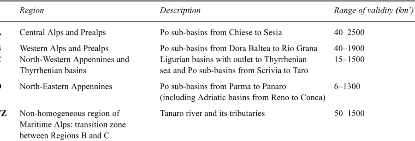
Region Description Range of validity (km2)
A Central Alps and Prealps Po sub-basins from Chiese to Sesia 40–2500
B Western Alps and Prealps Po sub-basins from Dora Baltea to Rio Grana 40–1900
C North-Western Appennines and Ligurian basins with outlet to Thyrrhenian 15–1500 Thyrrhenian basins sea and Po sub-basins from Scrivia to Taro
D North-Eastern Appennines Po sub-basins from Parma to Panaro 6–1300 (including Adriatic basins from Reno to Conca)
TZ Non-homogeneous region of Tanaro river and its tributaries 50–1500 Maritime Alps: transition zone
between Regions B and C
Fig. 11. Homogeneous regions and transition zone in north-western
Gupta, V.K. and Dawdy, D.R., 1994. Regional analysis of flood peaks: multiscaling theory and its physical basis. In: Advances
in Distributed Hydrology, R. Rosso, A. Peano, I. Becchi and G.
Bemporad (Eds.). Water Resources Publications, Highlands Ranch, Colorado. 149–168.
Gupta, V.K., Mesa, O.J. and Dawdy, D.R., 1994. Multiscaling theory of flood peaks: regional quantile analysis. Water Resour.
Res., 30, 3405–3421.
Hosking, J.R.M., 1986. The theory of probability weighted
moments. Research Report RC 12210, IBM Research, Yorktown
Heights. 1–160.
Hosking J.R.M. and Wallis, J.R., 1994. Some statistics useful in regional frequency analysis. Water Resour. Res., 29, 271–281. Kumar, P., Guttarp, P. and Foufoula-Georgiu, E., 1994. A probability weighted moment test to assess simple scaling. Stoch.
Hydrol. Hydraul., 8, 173–183.
IH (Institute of Hydrology), 1999. Flood Estimation Handbook (five volumes). Institute of Hydrology, Wallingford, UK. Lamperti, J., 1962. Semi-stable stochastic processes. Trans. Am.
Math. Soc., 104, 62–78.
Lovejoy, S. and Schertzer, D., 1990. Multifractals, univesality classes and satellite and radar measurements of cloud and rain fields. J. Geophys. Res., 95, 2021–2034.
Merz, R., Piock-Ellena, U., Blösch G. and Gutknecht, D., 1999. Seasonality of flood processes in Austria. In: Hydrological
Extremes: Understanding, Predicting, Mitigating, Gottschalk et al. (Eds.). IAHS Publ. no. 255, 273–278.
National Research Council, 1988. Estimating the Probabilities of
Extreme Floods: Methods and Recommended Research. Nat.
Acad. Press, Washington, D.C.
Natural Environmental Research Council, 1975. Flood Studies
Report, Vol 1, NERC London.
Pardé, M., 1947. Fleuves et rivières. 2 edn. rev. et corr. Colin, Paris.
Piock-Ellena, U., Merz, R., Blösch G. and Gutknecht, D., 1999. On the regionalization of flood frequencies - Catchment similarity based on seasonalitry measures. XXVIII IAHR
Proceedings, CD-Rom, 434.htm.
Potter, K.W., 1987. Research on flood frequency analysis: 1983-1986. Rev. Geophys., 25, 113–118.
Reed, D.W., Jakob, D., Robson, A.J., Faulkner, D.S. and Stewart, E.J., 1999. Regional frequency analysis: a new vocabulary. In:
Hydrological Extremes: Understanding, Predicting, Mitigating,
Gottschalk et al. (Eds.). IAHS Publ. no. 255, 237–243. Robinson, J.S. and Sivapalan, M., 1997a. An investigation into
the physical causes of scaling and heterogeneity of regional flood frequency. Water Resour. Res., 33, 1045–1059.
Robinson, J.S. and Sivapalan, M., 1997b. Temporal scales and hydrological regimes: implications for flood frequency scaling.
Water Resour. Res., 33, 2981–2999.
Schertzer, D. and Lovejoy, S., 1987. Physical modelling and analysis of rain clouds by anisotropic scaling multiplicative processes. J. Geophys. Res., 92, 9693–9714.
Sumner, G., 1988. Precipitation: process and analysis. Wiley, Chichester, UK.
Tasker, G.D., 1982. Comparing methods of hydrologic regionalization. Water Resour. Bull., 18, 965–970.
Turcotte, D.L. and Greene, L., 1993. A scale-invariant approach to flood frequency analysis. Stoch. Hydrol. Hydraul, 7, 33–40. Waymire, E. and Gupta, V.K., 1991. On lognormality and scaling in spatial rainfall averages. In: Non-linear variability in
geophysics. Scaling and fractals, D. Schertzer and S. Lovejoy,
(Eds.), Kluwer, Dordrecht, The Netherlands. 175–183. Wiltshire, S.E., 1986. Regional flood frequency analysis I:
![Table 1. Scaling parameters of E[Q k ] and β k [Q] of the AFS in North-Western Italy as clustered into four regions according to seasonality analysis.](https://thumb-eu.123doks.com/thumbv2/123doknet/14771500.591443/9.892.206.676.156.747/scaling-parameters-western-clustered-regions-according-seasonality-analysis.webp)