DOPPLER RADAR OBSERVATIONS OF AN OKLAHOMA DOWNBURST
by
Marilyn Mitchell Wolfson
B.S., University of Michigan (1979)
Submitted to the Department of Meteorology and Physical Oceanography in partial
fullfillment of the degree of Master of Science
at the
Massachusetts Institute of Technology
February 1983
0 Massachusetts Institute of Technology 1983
Signature of Auth
VI
DepartmenY of Meteorologyand Physical Oceanography January, 1983 Certified by FF Accepted by Kerry Emanuel Thesis Supervisor T S$flTUTEMT
U-'='dam
Ronald Prinn Chairman, Departmental Commitee on Graduate StudentsDOPPLER RADAR OBSERVATIONS OF
AN OKLAHOMA DOWNBURST by
Marilyn Mitchell Wolfson
Submitted to the Department of Meteorology
and Physical Oceanography on February 18, 1983 in partial fullfillment of the requirements for the degree of
Master of Science in Meteorology
ABSTRACT
Detailed Doppler radar observations of a thunderstorm along a cold front in Oklahoma on 13 April 1981 reveal the existence of at least one
"downburst". They indicate that the downburst, a small scale intense downdraft which hits the surface and causes high winds, is a strictly low level phenomenon. The distinctive "bow" radar echo appears to be caused by cyclonic rotation of the storm and the "spearhead" echo appears to be due to cell formation along an occluded gust front ahead of the main storm cell.
A new hypothesis for the thunderstorm downburst is suggested which differs from previous theories that rely largely on thermodynamic arguments. It is proposed that increased low level convergence due to
the thunderstorm outflow intensifies the ambient cyclonic vorticity which, in turn, induces the dynamic vertical pressure gradient responsible for the downburst.
Also, a technique for deriving the horizontal vector windfield from radial velocity measurements, using the constraints of irrotationality or nondivergence, is developed and tested. While the derived winds are not meant to indicate the real windfield, preliminary results show that they are more useful in inferring storm structure than simple contour maps of the Doppler velocity field.
Thesis supervisor: Dr. Kerry Emanuel
CONTENTS
1. Introduction...4
2. Review of Past Work on Downbursts...6
3. Overview of the Synoptic Situation...13
4. Doppler Radar Data Analysis...18
A. Plan View...18
B. Side View...36
5. Two Dimensional Wind Field from Single Doppler Radar...49
A. Three experiments...51
B. Discussion of derivedwinds...69
6. A New Hypothesis...75
7. Conclusions and Future Work...80
APPENDIX A...82
APPENDIX B...89
APPENDIX C...93
Acknowledgements...96
1. Introduction
The subject of this thesis is the downburst, a small intense downdraft at very low levels in a thunderstorm. Downbursts and the outflow of wind they cause at the surface are known to be responsible for several jet airplane crashes in the last ten years and there is some speculation that the July 1982 accident in New Orleans may also have been caused by winds from a downburst. The destructive nature of
downbursts and the high risk they pose to the safe operation of aircraft near thunderstorms make their accurate prediction a very desirable
goal. This will not be achieved, however, until the theoretical understanding of downbursts improves.
The 1982 Joint Airport Weather Studies (JAWS) observing experiment was organized in an attempt to gather data and learn more about
downbursts. The JAWS project took place around the Denver, Colorado airport where, in 1975, a downburst related aviation accident occurred. Many downbursts were detected but most of them were of the type now
being called "dry" or "cumulus" or "virga" downbursts. A distinction must be made between these and the "wet" or "thunderstorm" downbursts which are the subject of this study. The two phenomena are very
different. They are easy to distinguish: the former come from benign looking cumulus clouds over the high plains and fall through a very deep and dry subcloud layer and the latter are associated with
thunderstorms. Thunderstorm downbursts have been detected throughout the Great Plains and the Midwest, on the east coast, and in Florida, while the cumulus downbursts have only been reported over the high
5
In Chapter 2 of this thesis I review some of the past work on
downbursts including observations and proposed theoretical
explanations. Chapter 3 contains a brief overview of the synoptic situation leading up to the formation of the thunderstorm investigated here, and Chapter 4 contains a detailed analysis of Doppler radar data gathered while the downburst was occurring. Ten separate views of the storm at times no more than 7 and as few as 3 minutes apart during a 50 minute period represent better resolution than is available in any of
the past observational downburst studies. In Chapter 5 a new technique is tested for estimating the horizontal windfield from single Doppler radar measurements, and in the second section of that chapter some
features of the estimated windfields are discussed. Using the
observations as a guideline, a new hypothesis for the downburst is
developed in Chapter 6. Conclusions and suggestions for further work are presented in Chapter 7.
2. Review of Past Work on Downbursts
The word "downburst" was introduced in a paper by Fujita and Byers (1972) to describe the situation in which a thunderstorm downdraft becomes hazardous to the operation of jet aircraft. If the downdraft has a speed of at least 12 fps at 300 feet above the surface, which is
comparable to that of a jet transport following the usual 3* glideslope on final approach, and an aerial extent 800 m or larger, which is big enough to have a noticeable effect on the aircraft (Fujita and Caracena, 1977), then it qualifies as a downburst.
One may rightly wonder what the difference is between the downburst and the well known, well researched thunderstorm downdraft. At first Fujita (1979) thought that they were essentially the same but that, in
the same way a funnel cloud aloft is not called a tornado, a mid-level downdraft in a thunderstorm would not be called a downburst. The
definition was later refined when it was decided that the downburst must induce "an outburst of damaging winds on or near the ground" (Fujita and Wakimoto, 1981) where "damaging winds" refers to winds that can be
estimated on the F-scale (for which the minimum threshold is 18 m/s). These damaging winds can be either straight or curved but they must be
highly divergent (Fujita, 1981). Thus, even in its most recent and more meteorological definition, the term "downburst" is meant to signify a potential human hazard. Whether or not it also signifies a distinct phenomenon in the atmosphere is a matter of some debate, and one which will be investigated in the current work.
Much effort has been spent relating specific radar echoes to ground In the course of his
investigation of the airplane accident at JFK airport in June, 1975
Fujita (1976) associated damaging downburst winds on the ground with a
"radar echo with a pointed appendage extending toward the direction of the echo motion" which he called a "spearhead" echo. "The appendage
moves much faster than the parent echo which is being drawn into the
appendage. During the mature stage, the appendage turns into a major echo and the parent echo loses its identity."
After further observational work a more general type of echo with which downbursts were associated was identified by Fujita (1978) as the
"bow" echo which then takes the shape of a "spearhead" echo during the strong downburst stage and which sometimes develops a weak echo channel
in the area of strongest winds. There is some question as to whether
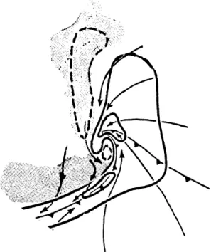
the downburst is simply associated with or actually causes these distinctive echo configurations. A schematic drawing of the bow echo evolution as proposed by Fujita is presented in figure 2-1 and radar
images of a confirmed downburst thunderstorm in Illinois are shown in
figure 2-2. Notice the cyclonic circulation north of the spearhead and
downburst where Fujita has indicated a tornado. An extensive ground damage survey of that downburst thunderstorm on 6 August 1977 in
Springfield, Illinois by Forbes and Wakimoto (1981) revealed many
downbursts, microbursts (downbursts with dimensions less than 4 km), and tornadoes. Their results consistently show the strong cyclonic
curvature and tornado paths to be on the north (left) side of the diverging wind pattern of the downbursts.
A study of radar intensity data associated with reports of
tornadoes by Nolen (1959) led to the identification of the Line Echo Wave Pattern (LEWP). The LEWP was defined as a "configuration of radar
Figure 2-1
Figure 2-2
Evolution of bow echo proposed by Fujita in 1979. In his model a bow echo is produced by a downburst thunderstorm as the downflow cascades down to the ground. Finally the horizontal flow of a weakening downburst induces a mesoscale circulation which distorts the initial line echo into a comma-shaped echo with a rotating head. From Fujita(1981)
W54
Radar pictures showing a bow echo which turns into a spearhead echo and then into a comma echo. During its spearhead stage,
this bow echo produced a cluster of 10 downbursts near Springfield, Illinois on 6 August 1977.(25 n mi range markers)
From Fujita, (1981)
TALL ECHO
BOW ECHO0 STAGE
COMMA ECHO STAGE
TOND SPA
' . OOWIMS '
echoes in which a line of echoes has been subjected to an acceleration
along one portion and/or a deceleration along that portion of the line
immediately adjacent, with a resulting sinusoidal mesoscale wave pattern in the line." There is a definite similarity to the bow echo and, in fact, Nolen found many examples of the LEWP which had associated reports of high winds but not tornadoes. Hamilton (1970) was able to deduce a
meso-low surface pressure area associated with the crest of the LEWP from the shape of the squall line as depicted on radar.
Fujita (1978) has documented downbursts associated with hook echoes, a distinctive configuration known to be a good indicator of at
least a mesocyclone and often a tornado. He has documented a series of
downbursts which all occurred on the south side of a mesocyclone moving
from northwest to southeast across the Kansas-Missouri border, he has
documented many twisting downbursts which show rotational as well as
divergent wind patterns, and he has even inferred the existence of a
downburst from the damage pattern left by a hurricane over land. It is
difficult to ignore these coincidental occurrences of downbursts with
strong cyclonic rotation. Yet most explanations for the downburst do exactly that.
Fujita (1976) and Fujita and Byers (1977) developed a model of the downburst thunderstorm which accounted for the spearhead echo. They proposed that the downburst is caused by the collapse of an overshooting
top on a large tall cell. The potential energy of the cloud top is converted into kinetic energy of the descending air which, by virtue of its large horizontal momentum, moves faster than neighboring parts of
The main downdraft in a mature thunderstorm is a result of the
cooling of dry mid-level air within the storm and/or the cooling of
sub-cloudbase air by evaporation. The downdraft produces an outflow of air beneath the storm, but the vertical velocities are weak when the cooled air reaches the surface. There is often a gust front at the edge of the outflow with associated wind shear and a dramatic temperature drop. The similarity between Fujita's proposed mechanism for downbursts and the mechanism known to produce the thunderstorm downdraft led some
scientists to the conclusion that Fujita was observing ground damage
caused by the gust front itself. As observations accumulated, it became clear that the gust front was one of the key ingredients but that the downburst was a smaller scale, separate phenomenon. Caracena (1978) suggests that a large downdraft may naturally contain an ensemble of small impulsive components of various intensities, and that downbursts and microbursts may simply be the stronger ones of these. He also notes
that they may occur more commonly than one might expect from the relatively few published case studies.
A study was done by Caracena and Maier (1979) of a microburst
associated with a thunderstorm which passed over the Florida Area Cumulus Experiment surface mesonetwork. They concluded that the
spearhead echo associated with that storm was "symptomatic of strong boundary layer forcing and moisture flux convergence". This, however, did not explain why or how microbursts occurred. The authors noted that a technique by Foster (1958), based on moist adiabatic descent of
downdraft air consisting of a mixture of midlevel air and updraft air, failed to account for the strength of the observed winds. They suggest
unmixed entrainment of environmental air into the rain shaft and/or the melting of a large quantity of precipitation".
Although downbursts come in many different sizes (Caracena, 1978; Fujita and Wakimoto, 1981) ranging from 1 km to 40 km with extremes of
0.1 km and 200 km, most documented thunderstorm downbursts are on the
order of 5 km across and are much smaller and stronger than the main downdrafts. This discrepancy led Emanuel (1981) to speculate that downbursts may be due to a dynamically distinct mechanism. He suggests
that downbursts are manifestations of the "penetrative downdraft" which
could account for their strength and small scale. The potential for penetrative downdrafts inside a thunderstorm exists when cool dry air overlies cloudy air of high liquid water content. The updraft
-downdraft configuration in a supercell thunderstorm may provide this setting. Emanuel is the first theoretician to suggest some connection between the storm rotation and the downburst although, in his scenario,
the rotation serves only to trap air of high liquid water content and small vertical velocity directly below a region of inflowing potentially cold air, thus setting up a conducive environment for the penetrative
downdrafts.
None of the aforementioned mechanisms have been demonstrated to be the actual cause of downbursts although they are all plausible. They do provide some suggestion of what to look for in the observations.
In summary, the recurring parts of the puzzle appear to be: a particularly strong cell within a line of thunderstorms; a bow echo or
LEWP in the mature stage of the cell; a gust front; some small scale rotation; decay of the parent cell as the echo shape begins to resemble
12
and a possible weak echo trench in the vicinity of the strongest winds. In these latter stages, the storm is decaying rapidly. The rest of this work will be concerned with trying to recognize these phenomena in the
radar observations of an Oklahoma thunderstorm and with understanding just how they combine to produce the downburst.
3. Overview of the Synoptic Situation
On 13 April 1981 during the National Severe Storms Laboratory
Spring Program a warm humid southerly airflow was present over Oklahoma, with a cold front oriented southwest to northeast moving into the state
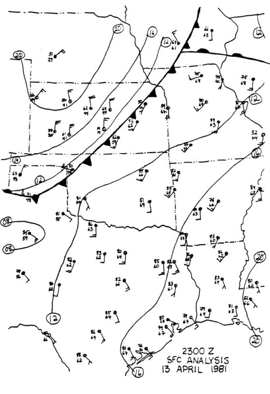
from the northwest. The surface analysis for 2300Z (1700 CST) or
approximately five hours before the front came into the Norman, OK area is presented in figure 3-1.
Temperatures in the warm sector were in the low to mid-eighties while dew points were between 60*F and 70*F. Temperatures in the air behind the cold front were considerably lower, ranging from about 70*F close to the front to the lower fifties well back into the cold high pressure region. Dew points in the cold air were correspondingly lower,
between 30*F and 45*F.
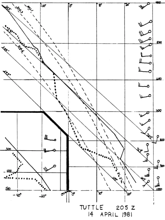
A sounding taken at Tuttle, OK (Tuttle is marked with a triangle in figure 4-2) shows warm moist surface air, a slight capping inversion at 850 mb and an approximately dry adiabatic lapse rate up to 500 mb
(figure 3-2). This sounding was taken at 2005 CST, an hour before the thunderstorm arrived, and is representative of the pre-storm
environment. The surface winds are light from the southwest but at slightly higher levels a southerly low level jet is present. The winds turn gradually to become more westerly and stronger with height.
The enhanced IR GOES-EAST satellite picture (figure 3-3) taken at 300Z (2100 CST) shows strong convection along the cold front. The most vigorous tall thunderstorms are located in Texas and on the Texas -Oklahoma border, while the cloudtops over -Oklahoma are basically
'0 2300 Z
SFC
ANALYSIS
15 APRIL
(981Figure 3-1 Surface map with all available stations plotted according to the conventional model. Temperatures and dewpoints are in OF. Isobars are labeled as the excess
(in mb) over 1000 mb. This map was an-alyzed and kindly made available by
TUTTLE
205 Z
14
APRIL 1981
Figure 3-2 (Plotted by
John DiStefano)
Tuttle sounding. The solid unlabeled line is the temperature sounding and the dotted line is the dewpoint sounding. Horizontal solid lines are pressure labelled in millibars and vertical solid lines are temperature in *C. Solid sloping lines are dry adiabats labelled in K and dashed
Figure 3-3 Enhanced IR satellite photo (MB curve) taken by the GOES - EAST satellite at 300Z on 14 April 1981
17
storm is blanketing and obscuring the tops of the weaker line of storms in Oklahoma. There is, however, some suggestion of a second point
source in OK where the anvil appears to bulge out and then become narrow again to the northeast. Because of the obscuring "blowoff" from the Texas storm there is no evidence of extreme cloud top warming (8*C, Fujita, 1978) during the downburst or cooling afterward, nor is there evidence of any large rapid changes in the areal extent of the anvil.
4. Doppler Radar Data Analysis
Much information can be gained by examining the reflectivity and radial velocity fields observed by the Norman, OK Doppler radar (NRO) while the downburst was occurring. A preliminary overview of the
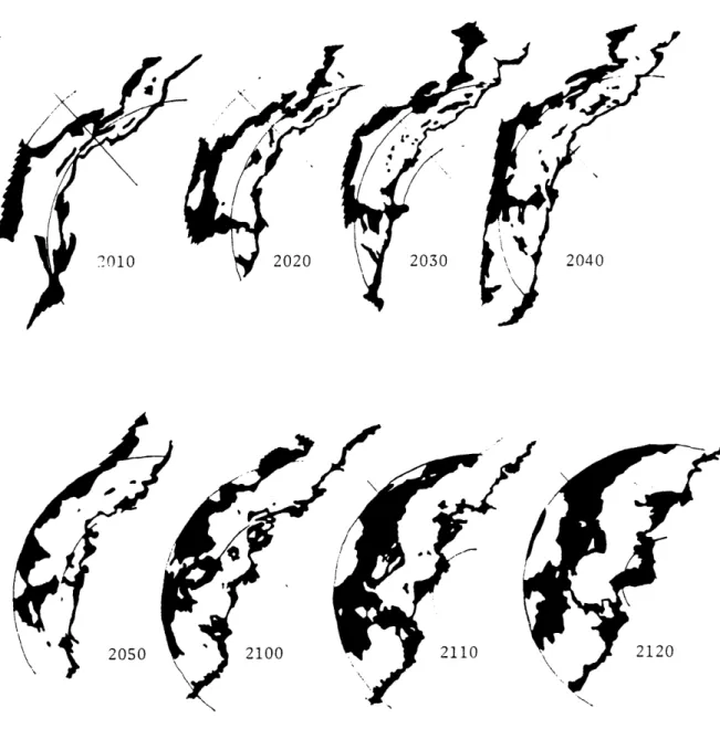
evolution of the line echo can be obtained from the Norman WSR-57 radar images (figure 4-1). This information is valuable because it often represents the only radar coverage of a storm and much of the literature on downbursts relies on this type of representation.
Notice that at 2100 CST a strong circular cell is present and the line has begun to protrude south of that cell. The echo has reached the "bow" echo stage. By 2110 the echo has entered the "spearhead" stage and the LEWP is evident.
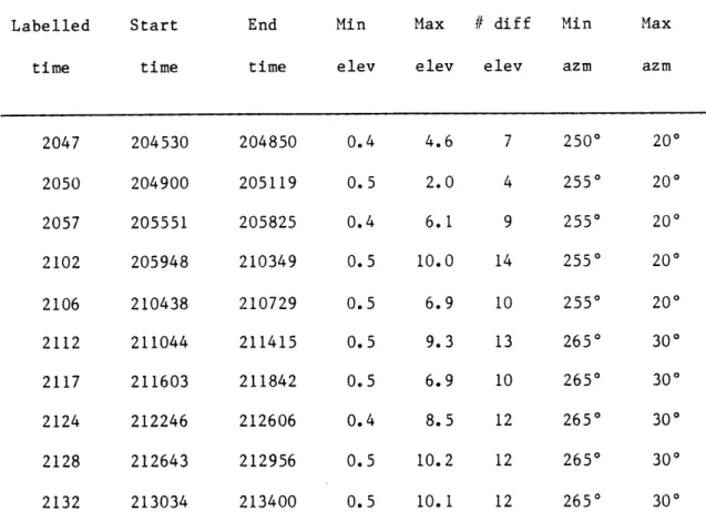
The results from NRO are extremely detailed in comparison with those from the WSR-57 radar. Ten tilt sequences were recorded during the fifty minutes between 2045 and 2135 CST and the rapidly changing nature of this storm required that all of them be analyzed. Details of
the available coverage and the data analysis are contained in Appendix A. The results are plotted on a 50 km2 grid in a Cartesian coordinate
system with the origin at NRO. Both the Cartesian and radial (radar) coordinate systems as well as the location of the storm at various analysis times are shown in figure 4-2.
A. Plan View
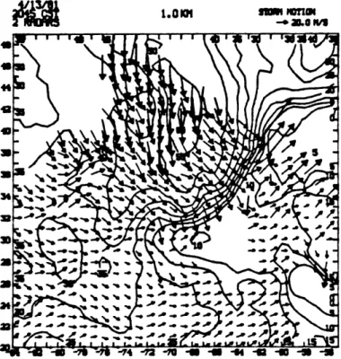
A series of maps showing the evolution of the reflectivity and Doppler velocity fields at 1.0 km above the ground is presented in
/A
2110 2120
(
Figure 4-1 Norman WSR-57 integrated received power at the times shown (CST) on 13 Anril 1981. These are
PPI displays at 00 elevation. The large arc in each picture is the 120 km range ring and the thin straight line is the 320' radial.
Figure 4-2 Depicted on the following page is the Norman, OK radar coordinate system used in displaying the analyses. The origin is at the Norman Doppler radar (NRO) and coordinates are labelled in km. The radials are labelled in degrees with 360* at duI north. The lower left hand corner of each 50 km box is marked with the time (CST) shown in that box in the following figures. The I symbol represents a Doppler radar, one of which
(NRO) is located at the origin and the other of which is Cimarron (CIM) located at 310* and 41 km from the origin. The two dashed boxed show the spaces for which the 2-Doppler analyses were at-tempted. The left box, 30 square kilometers in area, was chosen for the 2045 CST analysis and the right box, 15 square kilometers, was chosen for the 2130 CST analysis. The small dots located between NRO and CIM are the surface mesonetwork stations.
3150 3450
~80
70 300 - 60 so K) 40-.20
2047 205b 2C57 2002 2\)022102
- lo i10o s90 -s- -- 7 ~-0 -3'o -zbradial motion toward the radar.
The storm is very strong at 2047 CST and 2050 CST (figures 4-3 and 4-4) when reflectivity values greater than 55 dBZ can be found. Based upon analyses of much larger extent (not shown here) it is clear that there is a very well defined gust front oriented in approximately the east-west direction, as evidenced in figure 4-3 by the east-west line or arc of enhanced reflectivity which intercepts the right border at y=35. The gust front curves to become more parallel with the cold front
slightly farther to the east. This thin line echo is thought by
Wakimoto (1982) to be due to a "precipitation roll" which begins in the head of the cold outflow current. It may also be due to dust, insects, or a thermal discontinuity at the outflow edge. It is not clear which thunderstorm cell has produced the outflow responsible for this
east-west oriented gust front but it is probably a cell to the northeast of the one depicted in figure 4-3, or perhaps it is a number of
different cells along the front whose outflows have merged. There is another gust front present which is definitely due to the outflow from the depicted cell. It is oriented northeast to southwest and is
evidenced by the tight reflectivity gradient from 15 to 40 DbZ
(Wakimoto, 1982) on the southeast side of the high reflectivity core. In the following discussion I refer to these as two separate gust fronts although, as the cell evolves, this distinction becomes somewhat
artificial.
At 2047 CST there is a closed 15 dBZ contour on the east-west gust front. By 2050 this has grown to a 25 dBZ closed contour and at 2057 CST (figure 4-5) there is no longer any distinction between this region
considerably. The rapid growth of this cell was probably due to the increased convergence of inflowing air near the junction of the gust fronts. In a less detailed view, this behavior might suggest the
formation of a spearhead echo with the parent echo being drawn into the appendage. At the same time there is a southward protrusion and a
suggestion of cyclonic turning of the outflow air behind the north-south gust front. This motion is particularly evident in the -25 m/s "isodop"
(line of constant Doppler velocity) and in the increasing velocity gradient between 2047 and 2057 CST.
By 2102 CST (figure 4-6) the cell looks very different. The east-west gust front is still present and a new closed 15 dBZ contour has appeared. A "hole" has developed in the 45 dBZ contour behind the north-south gust front which corresponds to an increased area of maximum velocity toward the radar. The eastern portion of the -25 m/s isodop has become more rounded and extended southeastward while the northern edge has been deflected strongly southwestward suggesting a substantial increase in the cyclonic rotation. Note that the reflectivity field is less than 20 dBZ at the western edge of the depicted domain around y=25 and that a cell of greater than 45 dBZ is evident on the southern edge of the domain around x=-68.
At 2106 (figure 4-7) the "hole" in the 45 dBZ contour is still evident but the 40 dBZ contour has now protruded southeastward, and a small bullet shaped region of high radial velocities has developed in the same place. The east-west gustfront is characterized by a
reflectivity cell of greater than 25 dBZ. The outflow air behind the gust fronts appears to be merging, suggesting an occlusion process. The
grown and has curved in an anticyclonic sense, although this does not appear clearly in the Doppler velocity field. Notice, also, the anticyclonic "hook" in the 40 dBZ contour.
The downburst, .characterized by low 4e and maximum wind gusts, is known to have hit the surface mesonet station just south of CIM
(coordinates -30, 25) at 2110 CST (DiStefano, 1983). I suggest that the velocity maximum and 40 dBZ protrusion at 2106 are due to the
downburst. The reflectivity minimum or "hole" at 2102 appears to be related to the downburst and may be an indication of a newly formed updraft. Note that these features are quite distinct horizontally from
the dry region in the southwest.
At 2112 CST (figure 4-8) there is continued dry intrusion from the west and a suggestion of a "weak echo trench" or "spearhead trench" with
the spearhead being the deflection of the reflectivity contours probably due to the downburst. It is not at all clear that the dry air to the west and the spearhead are causally connected. The storm has weakened
greatly and even the 50 dBZ region is breaking up and shrinking in size. The lobe of high reflectivity extending southeastward with dry
(less than 5 dBZ) air behind it is the old east-west gustfront. There may actually be another downburst occurring at this time at x=-33, y=35 where the reflectivity minimum exists in approximately the same place
relative to the core of the storm and the gustfronts as did that at 2102 CST.
In the series of pictures from 2117 to 2132 CST (figures 4-9 to 4-12) the southeastern portion of the Doppler velocity field clearly
2047 CST -85 -88 -75 -78 -65 -REFLECTIVITY (DBZ) 2047 CST 1.0 KM -90 -85 -80 -7S -70 -65 -60 -55 -SO -45 DOPPLER VELOCITIES (M/S) 1. 0 KM
2050 CST -96 -85 -80 -75 -70 -65 -68 -55 -SO -45 -40 REFLECTIVITY (DBZ) 2050 CST
1.0
KM
-80 -75 -70 -65 -60 -55 DOPPLER VELOCITIES (M/S) 1.0 KM2057 CST
REFLECTIVITY (DBZ)
2057 CST 1.0 KM
IIII ldilil III pI I . .
-70 -65 -6e -55 -50
DOPPLER VELOCITIES (M/S)
2102 CST REFLECTIVITY (DBZ) 2102 CST 1.0 KM -6S -68 -SS -SO -45 -40 -35 -30 DOPPLER VELOCITIES (M/S) 4-6 i.0 KM
2106 CST -65 -66 -55 -50 -45 -40 -35 -30 -2S REFLECTIVITY (DBZ) 2106 CST 1.0 KM DOPPLER VELOCITIES (M/S) 1.0 KM
2112 CST 1.0 KM -65 -60 -55 -50 -45 -40 -REFLECTIVITY (DBZ) 2112 CST 1.0 KM -60 -55 -50 -45 -40 -35 -30 -25 -20 DOPPLER VELOCITIES (M/S)
2117 CST
-60 -55 -S -45 -46 -35 -30 -2S -20 -IS
REFLECTIVITY (DBZ)
2117 CST 1.0 KM
-50 -45 -40 -3S -30 -as -ae -is
DOPPLER VELOCITIES (M/S)
2124 CST
-Se -45 -40 -35 -30 -ES -20 -IS -10 -S
REFLECTIVITY (DBZ) 2124 CST 1.0 KM -50 -45 -40 -35 -30 -2s -20 -IS -10 -S DOPPLER VELOCITIES (M/S) Ie'L. -SS 1.0 KM
2128 CST -40 -3S -30 -25 -29 -IS -10 REFLECTIVITY (DBZ) 2122 CST 1.0 KM -45 -40 -3S -30 -2S -20 -iS -10 -S DOPPLER VELOCITIES (M/S) 1.0 KM
2132 CST -45 -40 -35 -30 -25 -20 -15 -10 -5 REFLECTIVITY (DBZ) 2132 CST 1.0 KM -45 -40 -35 -30 -25 -20 -IS -10 -5 DOPPLER VELOCITIES (M/S) 1.0 KM
4/13/81
2130 CST 1.OCKM' STORM MOTION
2 RADARS 20.0 M's 31 30 -. -- -191 28 40 N ttt
~
~
~
A A 27 - -1 - - - -26 - AA"AA 25HORIZONTAL~" F[L/WFET ,LW ,:-0;a 24 40 23 22 '0 21 A A--20ar A wins i 18 17 0 9 1 1 1 13 3G--21 -20 -19 -18 -17 -16 -15 -14 -13 -12 -11 -10 -9 -8 -7
HOPRIZONTAL FLCOA FEEID'?;L.CT .:: - Z
Figure 4-13 The 2-Doppler wind and reflectivity analysis for 2130 CST. The winds in the lower left portion of the domain could not be calculated accurately due to geometric factors.
in the partial wind field from the 2-Doppler radar analysis at 2130 CST shown in figure 4-13. (Details of that analysis can be found in
Appendix B). The weak reflectivity region in the west continues to grow and, by 2128 CST, appears to have infiltrated in an anticylonic manner what was the main core of the cell. The strong echoes in the southern region at 2102 (figure 4-6) have merged with the 40 dBZ region of the remnants of the main cell by 2124 (figure 4-10) and have become part of the "bow". Also, by 2124 the gust front structure is pretty much
destroyed. The cell along what was the east-west gust front has grown to 35 dBZ and merged with the main storm fragments by 2128 while the strong reflectivity gradient associated with the north-south gustfront has spread out completely.
B. Side View
Figures 4-14, 4-15, and 4-16 are displays of reflectivity and Doppler velocities on vertical east-west oriented surfaces through the storm at three times (2102, 2106, and 2112 CST) during the occurrence of the downburst. The surfaces are 5 km apart in the north-south direction from y=20 to y=50 with two extra surfaces added in the vicinity of the downburst (y=27 and y=33). The isolines intersect the lower surface vertically because the z=0 data is taken to be exactly the same as that at z=0.5 km.
At 2102 CST (figure 4-14) the storm is still strong, and
reflectivities aloft are greater than 55 dBZ at y=40 and y=45. The northeast-southwest orineted gust front is very clear in the lowest two kilometers from y=25 to y=40. At y=33 the vertical gradient of radial velocity is extremely intense at the front edge of the gust front. Note
the depression in the isodops between x=-45 and x=-50; the depth of the outflow layer is less at y=33 than to the north or to the south of that line. It was in this area that the "hole" appeared in the 45 dBZ
contour (refer to figure 4-6).
At y=40, north of the gust fronts, the outflow layer is very different. Notice the intense kink in the isolines of both plotted variables at z=2.5 km on the eastern edge of the high reflectivity core. This suggests the existence of a strong updraft around which I believe there to be cyclonic motion (see Chapter 5, section B).
Also of interest in figure 4-14(B) are the intrusions of dry air aloft into the storm from the west. These appear at very regularly spaced intervals in the vertical (every 2'km) and suggest a possible wavelike structure. This dry air certainly appears to be furthering the decay of the storm.
At 2106 CST (figure 4-15) a quick glance shows that the storm has noticeably decayed in the last 4 minutes. There are now no areas of reflectivity 55 dBZ or greater. At y=35 (figure 4-15(B)) the "head" of the outflow current is very pronounced. This is the area of the
occlusion where the gust fronts are merging and also appears to be a region of strong upward vertical motion, as evidenced by the Doppler velocities away from the radar. The downburst has hit the ground by this time as can be seen by the -25 m/s isodop at y=27 between the x-coordinates -40 and -35.
This picture at y=27 is interesting for another reason. Both it and the picture for y=25 below it show a distinct downward protrusion of
this stage the downdraft appears to penetrate to the 2 km level.
Judging just from the reflectivity contours, this formation looks very much like the vertical crossection from which Fujita (1979) postulated the descent of air from a caved-in overshooting top all the way to the ground. It is also possible that this is an example of the "penetrative downdraft" of Emanuel (1981). At any rate it is clearly separate from the downburst at the leading (eastern) edge of the storm and it appears to be aiding greatly in the rapid decay of this cell.
At 2112 CST (figure 4-16) the original downburst is evidenced by the -25 m/s isodop at y=25 and x=-35. From the surface analysis
(DiStefano, 1983) the downburst is known to have crossed x=-30,y=25 at 2110 CST. The time discrepancy is due to the use of the midpoint in time to characterize this entire tilt sequence. I suspect that another downburst has occurred at x=-33, y=35 because of the strong vertical isodop gradient, the accelerated patch of low level air centered around x=-30, and the "hole" or "notch" that has developed in the 40 dBZ
contour (refer to figure 4-8).
At this time as well there are downward protrusions of the
reflectivity contours, perhaps due to downdraft activity, occurring in every picture from y=20 to y=33. Notice at y=30 there might be a dry thermal (versus a plume) centered around x=-45, z=4.5. There is also evidence that some of this dry air has arrived at the surface.
The dry intrusion from the west is clear at the left edge of figures 4-16(A) and 4-16(B). Judging from these pictures this air is moving into the storm cell not only horizontally from the west but vertically from above as well.
Figures 4-14 through 4-16 each consist of 3 separate pages, each with 3 side views of the storm at the specified time. Heavy solid lines are isodops labelled in meters/sec. Negative values signify motion toward the radar. Shading represents the reflectivity field in DbZ according to the code below. The abscissa represents the east-west
direction and the ordinate, the vertical. Both axes are labelled in km in the NRO coordinate system. The y-coordinate of each picture is noted at the top of each frame.
REFLECTIVITY SHADING CODE
55 Db 50 DbZ 45 DbZ 40 DbZ 35 Db: 30 DbZ 25 DbZ 20 DbZ 15 DbZ 10 DbZ 5 DbZ
2102
CST
-80
-75
-70
-65
-60
-SS
-S
-4S
-40
-35
-30
2102 CST
Y =
25
-80
-75
-70
-65
-60
-S5
-S
-45
-40
-35
2102
csT
Y=
20
-30
I I I q 8-to ' , ' - -; 0-80
-75
-70
-65
-60
-55
-50
-45
-40
-35
-30
V = 27
2102
CST
V = 2710
8
6
4
2
0
10
2
6
4
2
0
-80
-75
-70
-65
-60
-55
-50
-45
-40
-35
-30
2102 CST
Y=
20
-80
-75
-70
-65
-60
-55
-50
-45
-40
-35
-30
2102 CST
Y = 25
-80
-75
-70
-65
-60
-55
-50
-45
-40
-35
-30
2102
OST
2102 CST
Y
=33
2102 CST
V
=30
2102 CST
-80
-75
-70
-65
-60
-SS
-S
-45
-40
-35
-30
2102 CST
Y
=45
2102 CST
y = 402
10
6
4
2
0
10
8
6
4
2
0
Y = 502106
CST
Y
= 27
10
4
6
4
2
0
10
8
6
4
2
10
6
4
2
0
-75
-70
-65
-60
5
-50
-45
-40
-35
-30
-25
2106
CST
Y =
20
-to-75
-70
-65
-60
-55
-50
-45
-40
-35
-30
-25
2106
CST
Y
=25
2106
CST
2106
CST
2106 CST
V = 33 Y =30
-75
-70
-65
-60
-55
-50
-45
-40
-35
-30
-25
10
6
4
2
0
10
10
6
4
2
0
V = 352106
CST
Y =
50
2106 CST
Y
= 45
-75
-70
-65
-60
-55
-50
-45
-40
-35
-30
-25
2106 CST
'/40
-75
-70
-65
-60
-55
-50
-45
10
8
6
4
10
8
6
4
2
0
10
8
6
4
2
0
2112 CST
-70
-65
-60
-55
-50
-45
-40
-35
-30
-25
-20
2112 CST
Y
=25
2112 CST
Y
=20
10
8
6
4
2
0
Y = 27
2112 CST
Y
=
10
4 .. ... 0.-5-4
4
-70 -6
-6-SO5
-45
-40
-3
30
-25
-20
2112 CST
Y=
33
10
-15
4
-1 -- - 2 - -1 - -- -- 2 -; -7-0*-70
5-5
2112 CST
V
3
10
0
2
;-w
40
0Zo -20--70
-65
-60
-55
-50
-45
-40
-35
-30
-25
-20
2112 CST
-70
-65
-60
-55
-50
-45
-40
-35
-30
-25
-20
2112 CST Y = 45-70
-65
-60
-55
-50
-45
-40
-35
-30
-25
-20
2112 CST
Y
= 40
-70
-65
-60
10
8
6
4
2
0
Y = 505. Two Dimensional Wind Field from Single Doppler Radar
In the last fifteen years, Doppler radar has proven to be a very useful tool for investigating storm scale meteorological phenomena. Horizontal wind fields have been successfully and accurately derived using two or more Doppler radars simultaneously. A single Doppler radar can only detect the radial component of the wind field; it does this, however, very accurately and with a resolution of better than one kilometer. Yet it is often the case and will more often be the case when NEXRAD is fully implemented, that data from only one Doppler radar is available for a storm. Since it is very desirable to obtain the full vector windfield it is not surprising that quite a few studies have been done which try, using various additional assumptions and hypotheses about the flow, to derive the two dimensional windfield from detailed single Doppler velocity data.
By far the most common assumption made is that the flow varies linearly around its value at a given point. If the data are collected around a full circle at each elevation angle (Velocity Azimuth Display) the magnitude and direction of the horizontal wind (Lhermitte and Atlas,
1961) as well as the mean convergence and stretching and shearing
deformations (Caton, 1963; Browning and Wexler, 1968) can be derived. These techniques have been extended to conical sectors (Easterbrook,
1975) and full volumes (conical sectors or circles at more than one
elevation angle) of radar data (Waldteufel and Corbin, 1979), but always the analysis involves the simplifying assumption of linearity or of harmonic variation in space, in which case a highly truncated Fourier series is used to represent the mean wind. These approximations may be
applicable to stratiform rain situations but not to small scale severe
storms. The extreme smoothing inherent in those assumptions removes exactly the features of interest.
Another assumption that can be made is that the flow is unchanging in a reference frame attached to the storm. Then scans at different
times can be treated as simultaneous scans of the storm by two or more Doppler radars. This could only work if the storm was extremely fast moving so that the time separation between scans was small but the
difference in the mean direction of the storm from the radar was large.
This technique could not work for a rapidly evolving, rather slowly
propagating storm such as the one presented here.
In this thesis a different approach will be taken in deriving the two dimensional horizontal wind field. It can be easily shown
(Holton, 1972, Appendix C) that any vector V can be written as
where V is a nondivergent vector satisfying
V
V
0
(2)
and V is an irrotational vector satisfying
The radar measures the radial velocity component in spherical
coordinates. This is converted to the radial velocity in cylindrical coordinates by first taking at every point the horizontal component of the Doppler velocity (very close to what is actually measured at low
elevation angle) and then interpolating the measurements onto surfaces of constant height. (See Appendix A for more details). Thus the
horizontal wind field in cylindrical coordinates is
AA
V
Ve)
ke
4+
V
k
R.(4)
where VR is the known radial component, Ve is the azimuthal
A A
component to be derived, and ke and kR are unit vectors in the azimuthal and radial directions, respectively.
Expanding the right hand side of (1) into polar coordinates:
V
V"
er
X
[4
vK
(5)
A. Three experiments
Three different experiments have been performed. The first
experiment makes the assumption that the observed flow is irrotational
(VND=O). Thus
R -
Va(6
VZOSEKED R k(6)
R
(7)Now the angular derivative of V can easily be calculated at all
points in R and 8. Since only the radial derivative of the unknown VX appears in (7) the partial derivative will be an ordinary derivative along a line of e=constant. Multiplying by R, (7) can be rewritten
~~R
LR6
( i
(8)
along
9=-@
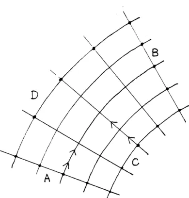
, where 80 is a radial line and is the known angular derivative of V. which can be thought of as a forcing function. The integration is a simple "marching" problem and requires only oneboundary condition. I have chosen to specify V at the inner line of constant radius, labelled C in figure 5-1, and integrate away from the radar. Alternatively, one could specify Vg on line D in figure
5-1 and integrate toward the radar, although because the flow appears to
be more quiescent along C it may be easier or less crucial to guess at the boundary condition there.
The second experiment makes use of the assumption that the observed windfield is nondivergent (Vn =O). Now the observed radial flow is defined as the radial component of the nondivergent flow. This flow will satisfy (2) which, with an assumed boundary condition, defines V Following a similar line of reasoning to that used in deriving (8), the equation to be integrated in this experiment is
Figure 5-1 The polar grid used in deriving Vg. Integration proceeded from A to B along lines of constant radius and from C to D along radial lines.
where R0 is a line of constant radius. V was specified along A in figure 5-1 and the integration was done clockwise along lines of constant radius. Again, the integration could have been started along B and proceeded counter clockwise.
The boundary condition used at all altitudes shown in both experiments was a 6 m/s southerly wind chosen to correspond to the synoptic scale flow in the prestorm environment. This condition was imposed on V. only; in all cases the observed V was used.
Calculations of the horizontal divergence and the vertical vorticity of the 2-Doppler derived winds at 1.0 km are presented in figure 5-2 for the 2045 CST windfield (figure 5-4) and in figure 5-3 for the 2130 CST windfield (figure 4-13). They show that the low-level
flow, at least at these times, is both rotational and divergent; the
vorticity and divergence of the actual windfields are roughly
comparable. Calculations by Ray (1976) of the vorticity and divergence in tornadic storms also show this to be the case. Thus the assumptions that the observed flow is either irrotational (experiment 1) or
nondivergent (experiment 2) are clearly both wrong. The premise behind
the third experiment is that they are wrong by roughly the same amount, that is, that they represent two extremes between which the real flow
lies.
The third experiment, then, combined the first two to make a more
2045 CST N>o -84 -82 -80 -78 -76 -74 -72 -70 -68 -66 -64 -62 -60 -58 -56 -54 DIVERGENCE (10-3 S-1) 2045 CST 1.0 KM 48- 46-44 42- 40- 38- 36-34 38-30 -00 28 24-0 -84-82 -80 -78 -76 -74 -72 -70 -68 -66 -64 -62 -60 -58 -56 -54 VORTICITY (10-3 S-) 1-0 KM
1.0 KM
!1-29-19-18-17-16-15-14-13-12-11-10 -9 -8 -7 -6
DIERGENCE (10-3 S-')
! -28-19-18-17-16-15-14-13-12-11-1S -9 -8 -7 -6
4-
VR
V
6.
-
/
LV
(10) Actually, this windfield is not realistic either; a windfield simulated in this way would correspond to the actual windfield only if the flow were everywhere constant. (In that case the division of the flow intoirrotational and nondivergent components would be nonunique and basically useless.)
Features of the "NONDIVERGENT" and "IRROTATIONAL" windfields shown in figures 5-6 through 5-13 will not be discussed in detail although I do think they are worth examining. The windfields derived in the third experiment are presented and discussed in section B of this chapter. Even though they are known to be unrealistic, I believe that the results
of the third experiment are more useful for recognizing characteristic flow patterns and inferring storm structure than simple contour maps of Doppler velocities, and that they qualify as valuable observational
tools. Before the discussion of these windfields, however, a few more comments on the accuracy of these experiments are in order.
Accuracy
It is very difficult to get an estimate of the accuracy of the irrotational versus nondivergent assumption. A very rough qualitative comparison can be made at 2047 CST, at 1.0 km, between the partial
windfield from the 2-Doppler analysis (figure 5-4) and the derived winds from single Doppler radar (figure 5-6). Notice that these latter wind fields are shown in 50 km2
boxes while the 2-Doppler winds are shown in 30 km2 boxes. (Appendix B contains more information on the
2-Doppler analysis.) Also, the reflectivity field is contoured every 10 dBZ but is unlabelled in the displays of the single Doppler winds. The values of reflectivity can be found by referring to the figures in chapter 4.
At least in this limited area it appears that the nondivergent approximation is somewhat more realistic than the irrotational approximation. It captures small scale (5 km) wavelike changes in
windspeed and direction which are probably real. However, the divergent outflow and in particular the northerly component of the wind is better captured in the irrotational windfield. Figure 5-5 is included for comparison although it is known to contain unacceptably large errors in all but the lowest third of the diagram. Again, the resemblance to the nondivergent flow is qualitatively stronger than to the irrotational flow. This may be partly because the synoptic scale flow itself is quasi-nondivergent.
The accuracy of the boundary condition and of the numerical
integration scheme also needs to be considered. As was stated earlier, the sensitivity of the derived windfield to the boundary condition on Ve is small. A boundary condition of Ve=0 was imposed and the flow was compared with that derived using a boundary condition of Ve=6 m/s. The influence of the boundary condition was apparent close to the boundary but was negligible more than 10 to 15 km away. Thus the
boundary condition will not cause large errors if it can be applied where the flow is either known accurately or where it is basically featureless. There is, however, a trade-off. Removal of the boundary from the vicinity of the depicted flow lengthens the path along which
4/13/81 204S CST 2 RADARS I ' ' ' ' 40 ' 1.00KM
q
- A5
\~ ~-~E ,p - - ~ -. - -STORM MOTION - 20.0 M/SIQ--A .- --84 -82 -80 -78 -76 -74 -72 -70 -68 -66 -64 -62 -60 -5 -56
HORIZONTn, FLOW F1EL0/REFEECT'T7y (08Z
Figure 5-4 The 2-Doppler wind and reflectivity analysis for 2045 CST. The winds in the upper portion of the domain could not be calculated accurately due to geometric factors.
1.00M sum MonM
-0 -0 P . 3.0 "NAl
tot!ZmWL
nL.0 FIE./RErCTIvT toz)Figure 5-5 The 2-Doppler wind and reflectivity fields from a trial run. All but the lower third of the diagram contains errors known to be unacceptably large. This picture is included for qualitative consideration only.
IT I I .NI \41\ 4IlQ N) K:D UD) : C t t ' ' 4 I t
11
TT' rt' TlI i tt-ir i \ -IJ~ I T I, 61t,v~
'o
4ILr fttN
'00 110 in in q U U2106 CST -ss -e -s -se-4S -40 IRROTATIONAL WIND 2106 CST 1.0 KM -+0 20 M/S as
K:Z--7s -70 -6s -e - -5e -4S -40 -3s -3o NONDIVERGENT WIND 1.0 KM -*0 20 M/S
1.0 KM -0 20 M/S -- a 6 -- & "a '_ I 30- -N- 25- 0-70 -65 -60 -55 -50 -45 -40 -35 -30 -25 -20 IRROTATIONAL WIND
i.e KPI -. 20 II'S
'is '~Ih ~5 'is". \ '~ Na Na ~' ~ Na "IS "S "S -~ ~ ~ Na Na N -' ~-m-~-'--- -'--U .-...- -.. ' .-- e--4--+ -.. ....- ..- V..* -55 -5O -45 -40 -35 -30 -25 -20 NONDIVERGENT UIND 2112 CST 2112 CST
2102 CST 2e -' 14 1 'a "~ a "a '~Ns "a -80 -75 -70 -65 IR 2102 CST 1.5 KM -- 20 I/S -60 -55 -50 -45 -40 -35 -3 ROTATIONAL WIND 1.5 KM -- 20 o'S 60 . . - - -. ... -.. "a " a - - +---- -' . -. -. --.-S-.-. - -' -45 3s5--0 - - -7 -es -60 -s5 -se -45 -40 -35 -30 NONDIVERGENT WIND e -% % % , Y,
-,. --..
%2112 CST 1.5 KM - 20 M/S cc %a %4 %4 ' 6No 5- -
~
N-
'
-45 40- --Na N N,' \6 1% ' 35- -a 30- I.& a -A 25 "a 20 -70 -65 -60 -55 -50 -45 -40 -35 -30 -25 -20 IRROTATIONAL UIND 2112 CST 1.5 KM -+ 2 M/S 5 35 -" ' "'a.A ' 5 - - 1' 1' 1~ 1' 1S 1 (1 a i- ' ' " ill r[ -t " L. I 50 - - --""~ ~
- wA 2 - - - - .--- -- S"a- . -Figure 5-11 'm Az -~~
-* ''S -. "s A 35 -' '.---* -. - -W -4P -W -. 15 Lj I"' I I I I - 7 -70 -65 -60 -55 -50 -45 -40 -35 -30 -25 -20 NONDIVERGENT U.INDai0 CsT 2.5 KM -- 20 /S 60-,
~
. se 45 40-3S -aso "e- 'a a a a a a a- a ' ' a 4 0 . . .U .a .a ' . '.. is- I . --30 -7s -70 -6s -6e -55 -50 -45 -40 -3S -30 IRROTATIONAL. IND ssF'
.~-.
--- 9pt 4 S 40--- ' * -- A 4. 0. -.-30' 0- E5--8e -7S -70 -GS -6 -SS -se -4S -40 -3S -20 NONDIVERGENT ,IND2112 CST 2.5 KM -+ 20 M/S -t * -60 -S -50 -45 -40. -35 -30 -25 IRROTATIONAL WIND 2112 CST 2.5 KM 2- ao s - * -lb? -65 -60 -55 -50 -45 -40 -35 -30 -2S NONDIVERGENT WIND 15 La -70 30 -25 20 -70 -20 -4
Accuracy in this numerical integration is indicated by how close the derived flow is to being either irrotational or nondivergent as the case may be. A test was performed using the radial component of a known divergent windfield and the constraint of irrotationality to derive the azimuthal velocity field. As one would expect, the errors were all in the azimuthal direction and they increased approximately linearly away from the boundary. The magnitude of the error was- 20% of the magnitude of the wind at the end of the integration path.
If the boundary conditions are known fairly accurately, then the numerical accuracy can be improved by integrating first in from one boundary and then in from the opposite boundary. The results could be
combined using the integrated value with the least numerical error as the true value at each point. This procedure has not yet been tested.
Before any real assessment of this entire technique can be made it must be tried on radar observations of a windfield that is known in detail from a multiple-Doppler analysis so that an extensive and quantitative comparison can be made.
B. -Discussion of derived winds
Although the results from the "nondivergent" experiment at 2047 CST appear closer to the actual winds from the 2-Doppler analysis than the "irrotational" winds, my best estimates of the actual wind fields are those from the combined irrotational and nondivergent experiment and they are the only ones that will be discussed here. These are meant simply to give a qualitative picture of the flow and features mentioned below must only be considered heuristically. It is somewhat instructive to turn back to the pictures in the previous section showing the