Development of utility system simulation model : progress report no. 2

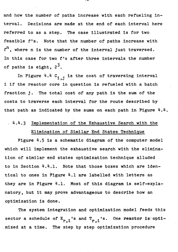
Progress Report No. 2

DEVELOPMENT OF UTILITY SYSTEM SIMULATION MODEL Period Covered: January 1, through June 30, 1971

Edward A. Mason Paul F. Deaton Joseph P. Kearney Terrance A. Rieck

DEPARTMENT OF NUCLEAR ENGINEERINO MASSACHUSETTS INSTITUTE OF TECHNOLOGY

CAMBRIDGE, MASSACHUSETTS

MIT DSR Project 72107

Work Performed for

COMMONWEALTH EDISON COMPANY CHICAGO, ILLINOIS

MITLbr-res

DISCLAIMER OF QUALITY

Due to the condition of the original material, there are unavoidable flaws in this reproduction. We have made every effort possible to provide you with the best copy available. If you are dissatisfied with this product and find it unusable, please contact Document Services as soon as possible.

Thank you.

The images contained in this document are of

the best quality available.

Section Title Page 1.0 Summary

2.0 Introduction 3

2.1 Background 3

General Direction of Work Accomplished and 3 and Planned

3.0 System Integration and Optimization 9

3.1 Introduction 9

3.2 SYSGEN, MIT's Version of the Booth-Baleriaux 9

System Model

3.3 Comparison of SYSTEN and SYSSIMUL 12

3.4 Optimization Model 18

3.5 Compatibility 21

3.6 Sensitivity Study 26

4.0 The Nuclear In-Core Simulator and Optimizer 2B

4.1 Introduction 2

4.2 The MOVE Code .31

4.3 The Proper Selection of Refuel Enrichments 36

4.4 The Optimization Procedure 37

4.4.1 Introduction 37

4.4.2 The .Nature of the Problem 38

4.4.3 Implementation of the Exhaustive Search 42 with the Elimination of Similar End

States Technique

4.5 Summary 45

5.0 The Engineering Feasibility and Fuel Cost 46 Analysis of Variable Nuclear Fueling Intervals

5.1 Summary of Proposed Work 46

5.2 Present Progress 47

6.o Methods -for Evaluating Worth and Marginal Costs 49 of Nuclear Fuel

7.0 Fuel Depletion and Costs During the Transient 52 Period of. the Zion Reactor

Appendices

A Thesis Prospectus - T.A. Rieck 65

B Thesis Prospectus - H.Y. Watt 72

C SYSGEN Code 80

D MITCOST Code

Considerable progress has been in the last six months of work sponsored by the Commonwealth Edison Company at MIT in the development of information and models useful for nuclear utility systems planning.

The present work is mainly divided between four doctoral candidate graduate students, three of whom are working

specifically on development of scheduling, physics, and

economic models. Together with maintenance scheduling model-ling work underway at Edison, these models will form a

complete system for multi-year planning for both Edison system generation schedules and nuclear fuel purchasing for existing nuclear units. The fourth student has started a technical and economic sensitivity study of various means of achieving variable length irradiation periods between reactor refuelings.

The first version of a rapid, versatile, multi-unit, multi-period generation scheduling computer code, SYSGEN,

employing probabilistic treatment of load forecasts and

forced outages has been prepared and tested. The code compu-tes expected energy production, capacity factors, fuel require-ments, and production costs for each unit for each period and also predicts the expected system non-serviced energy and loss-of load probability.

Detailed three dimensional calculations of the performance of the Zion Reactor, assembly-by-assembly, for the first nine

irradiation cycles from startup to equilibrium, have been

were compared to the results calculated using the CELL-MOVE fuel depletion and management code. CELL-MOVE, which has been developed on a period of years at MIT, has been under study and modification as part of the Edison project at MIT. CELL-MOVE is a rapid, simple code which will form part of the in-core simulator model to which forms pait of the over-all system model under development at MIT.

A rapid fuel cycle cost calculation code, MITCOST, has been developed. Cost calculations for the nine cycles (17

fuel lots) of the Zion approach-to-steady-state were performed using MITCOST, and several sensitivity studies of the Zion Reactor using CELLMOVE were performed.

Work on nuclear utility fuel and systems analysis con-tinues to be a growing area of graduate student interest in the Department of Nuclear Engineering at MIT. Work connected with the Edison contract now serves as a focal point for

much of this interest.

In addition to sections describing each of the major work areas, code descriptions and FORTRAN listings of SYSGEN and MITCOST are included as appendices.

2.0 INTRODUCTION 2.1 Background

This is the second progress report on work carried out for Commonwealth Edison Company.under a research contract with the Department of Nuclear Engineering at the Massachusetts Institute of Technology.

The objective of this research program is to assist Commonwealth Edison in developing techniques and information useful in the optimal planning and operation of the nuclear generating units in. their system. The work is accomplished by-graduate students, carrying of by-graduate thesis research, under

the supervision of Professors Edward A. Mason and Manson Benedict.

The results of the first year's work (calendar 1970) were summarized in Progress Report No. (1), by thesis reports

(9, 102, 11, 12, 15) copies of which have been sent to Edison and by two papers presented in November 1970 (13 ,14).

2.2 General Direction of Work Accomplished and Planned

The work carried out in the first half of 1971 and propo-sed for the coming year will be outlined using reference to Figure 2.1, Nuclear Power Management Multi-Year Model. The work has concentrated on developing a multi-year model (5-10 year planning horizon). Edison personnel have been working on the development of a sub-model for maintenance and refuel-ing schedulrefuel-ing of conventional and nuclear units subject to the -various system constraints, Blocks (1) and (2) on Figure 2.1.

Figure 2.1 Nuclear Utility Management -Multi-Year Model

To facilitate simultaneous development of several of the sub-models required by the various function blocks represented on Figure 2.1, the work has been divided into several areas with one graduate student working in each area. Linking between the various areas (and blocks) is accomplished by

careful definition of the type and form of information to be transferred into and out of each of the functional blocks. Not only does this facilitate independent development of sub-models at MIT, but will permit the use of sub-sub-models which may be developed by others (such as Edison and others in the

Joint Systems Analysis Task Force) and the replacement of the original sub-models with improved versions when produced by anyone.

MIT has been working for varying degrees of time in developing models and information useful for the remaining blocks on Figure 2.1. Paul F. Deaton, who has been supported by a Hertz Fellowship, is developing models fpr system inte-gration and optimization consisting of: a means for schedul-ing the production of all units, Blocks (3) and (4); calcula-ting total system costs, Block (9); and seleccalcula-ting the schedule with minimum total cost, Block (10). Refer to Section 3.0 of

this report for a summary of the progress on this part of the MIT program.

Joseph P. Kearney, who is supported as a Research Assis-tant under the Edison contract with MIT, is developing rapid nuclear in-core simulation and optimization models to be used

to accomplish the functions indicated by Blocks (6), (7), (8), and (9) of Figure 2.1. A summary of his progress is contained in Section 4.0. It is presumed that the actual nuclear fuel cost data,. Block (5), fuel cycle cost data, Block (7), will be supplied by Edison; for model development purposes fuel and cost data previously developed at MIT will be used in the form generally employed by reactor vendors and analysts. For simulation model checkout and sensitivity studies, Edison reactors are being employed as the examples.

Block (8) will use REFCO, a fuel cycle cost calculation code developed by Oak Ridge National Laboratory (16) and MITCOST a similar code recently developed at MIT by D.F. Martin and

J.C. Conklin (7). J. Conklin is in the process of completing a master's thesis, supervised by M. Benedict and E.A. Mason. His study has developed information concerning the fuel burn-up and core power distribution, assembly-by-assembly in the Zion 1 Reactor for the various cycles from startup to steady

state. Fuel cycle costs have also been calculated. The results of his work are of interest in showing how the Zion fuel can be operated to remain within the license restrictions

regarding power density and the fuel cost structure during the approach to steady state. In addition MITCOST is a very rapid

code for calculating batch-by-batch or period-by-period fuel cycle costs. A summary of Conklin's results is presented in Section 7.0. A description of MITCOST and a FORTRAN listing is included in Appendix D.

A comparison of the features and time and cost of operation of REFCO and MITCOST for calculation of fuel cycle costs will be made at MIT in the near future.

Another graduate student, Terrance A. Rieck, who is supported by an AEC Fellowship, has recently started thesis research associated with the Edison program at MIT. He will be making a detailed study of the engineering feasibility and fuel cost analysis of variable nuclear fueling intervals for a PWR. A summary of his plans and work to date is given in

Section 5.0; a copy of his Thesis Prospectus (3) is included as Appendix A. This work will provide a fast multi-group

depletion code which will be very useful in checking, and normalizing, the faster but more approximate in-core simula-tor under development by J.P. Kearney. Rieck's code could also be used as an in-core simulator if and when greater

accuracy and detail than proceeded by Kearney's model are re-quired. Furthermore, Rieck's work is aimed at defining the limits of feasibility, both economic and engineering, for the use of variable batch enrichments and size in achieving variable

irradiation times between required nuclear refuelings.

It should be noted that the work undertaken by Rieck was originally included in the general scope of the original thesis

prospectus of J.P. Kearney (2). However, as discussed in Sec-tion 4.0, Kearney's work on the development of an in-core

simulator precludes his carrying out detailed sensitivity studies as well.

A fourth doctoral candidate, Hing Yan Watt, who hopes to be supported as a Research Assistant under the Edison

con-tract, beginning September 1, 1971, has proposed to undertake the development of methods for evaluating worth and marginal costs of nuclear fuel. A brief summary of his research area is given in Section 6.0; a copy of his Thesis Prospectus (4) is included as Appendix B. Successful completion of this proposed study would probably lead to modification of the present concept of Blocks (6) and (8) on Figure 2.1 resulting in much more efficient and rapid optimization of nuclear fuel reload design and selection. Watt's work will be more in the area of the application of economic and reactor theory than in detailed model development; in this source the work, and results are expected to be similar to those of Hans Widmer (15), but with the simplifying restrictions of Widmer's pione-ering work removed.

In addition to the plans outlined above, an Italian engineer, Alessandro Ovi, will be entering the Department of Nuclear Engineering at MIT this fall with the express purpose of taking courses in operation analysis and doing research in nuclear power systems planning with E.A. Mason. He has a master's degree in nuclear engineering and has

worked for over a year in industry performing simulation and optimization studies. He will be supported by a Fullbright Fellowship.

Interest in the area of nuclear fuel and power manage-ment at MIT is growing, and it is expected that other

graduate students will elect to work in this area during the coming year.

3.0 SYSTEM INTEGRATION AND OPTIMIZATION (P. F. Deaton) 3.1 Introduction

As discussed in the first progress report (1), the System integration and Optimization module of the nuclear power manage-ment multi-year model will perform those tasks illustrated in Figure 3.1. The model's purpose will be (1) to integrate the plant characteristics of the utility into a viable model which meets the necessary operating constraints and (2), apply

optimization techniques to this model to yield minimum total system cost.

During the past six months, considerable progress has been made at MIT in establishing a first-generation integrated system model. Furthermore, a great deal of crystallizing of thought has occurred in the area or system optimization, but the real work of implementing those ideas is the major task that lies

ahead.

3.2 SYSGEN, MIT's Version of the Booth-Baleriaux System Model In mid-February, the Commonwealth Edison Company sent MIT a letter (5) strongly advocating the inclusion of the

Booth-Baleriaux model as "a firm part of the multi-year model". Later, a copy of SYSSIMUL, the TVA-ORNL computer model adapted from Booth's work (6) while with TVA, was sent to MIT for evaluation and comment. Even the preliminary evaluation indicated that the Joint System Analysis Task Force's interest in the Booth-Baleriaux model was wholly justified. The Booth-Baleriaux probabilistic approach to simulating utility operation was far and away the best model available.

NUCLEAR POWER MANAGEMENT MULTI-YEAR MODEL 7t

F-7

-Refueling and-- Sc eduling Constraints MaintnanceMai nt. Requir'ements

u

Alternat. Fu1Cost Estimates

Fo eced Outage Rates - -Valve-Point Info-.

Startup & -Shutdown Cps s Fuel Contract- Cons'tr.

TtlNudl Sched.. Nuc es

--Production Feas ib le Ener. Re d. Sch _ an Check_-for -Each.Faiblt Period -7 : -r i l Z i 4_- No-ucear EEstimate

-- Minimu YeBove detter Set.

Oper.- Cost _{of E IS.}

No eleect- Scheaule sIth Minimum Total Cost E s & T's, Energy- & -Length of. Each Cycler -4 *~1

* 1.2

2

4±j

IH

K

Iuclear Fuel Cost Data

- 7

Core lSimulation to

Optimize Nuclear Fuel Des igns

C C Optimum Reload Fuel: - Enr.chment Batch Size Min.'Tot.Cost

-

L2j7z

I Non-Nuclear !. Minimumi Fue Requirements Oper.. Cost, j mer, _{n g.} Purc rl-, - 7-e Total Syst-en Cost More Alternatives -? Total Cost

for -Each STO

The detailed evaluation that followed pointed out, however, that the TVA-ORNL adaptation of the model had many shortcomings. SYSSIMUL was:

(1) incorrectly coded, e.g., wrong loading chosen for the plants and costs calculated improperly,

(2) inefficiently coded, e.g., processed much zero or near-zero data,

(3) poorly coded, e.g., subroutine too long and performed too many functions (not modularized) and indexing ambiguous , and

(4) grossly misrepresenting loads and equivalent loads as being alternately flat and non-continuous ("stair-step"

shaped).

With these and other shortcomings in mind, a completely new version of the Booth-Baleriaux model was written here at MIT, and named SYSGEN (for SYStem GENeration) to distinguish it from SYSSIMUL. SYSGENts characteristics include:

(1) correct and efficient programming,

(2) loads and equivalent loads are treated as linearly continuous functions,

(3) calculation proceeds in a forward direction as opposed to SYSSIMUL's backward direction,

(4) allowance for up to 5 valve points per unit,

(5) inclusion of startup and shutdown costs and emergency power purchases to cover energy not served directly,

(6) inclusion of a spinning reserve requirement as it

costs and starts them up according to the input startup order,

(7) modularized input (See Figure 3.2) allows one computer run to perform calculations for up to 100 consecutive periods, under any number of complete beginning-to-end refueling and maintenance strategies (that is, 100 periods under Strategy 1 followed by same 100 periods under Strategy 2, etc.) and,

(8) more complete output (See Figures 3.3, 3.4, and 3.5)

giving not only gigawatt-hours of electricity produced, but also millions of BTU (MEGABTU's) energy consumed by each unit.

Later versions will also include forecasting errors, peak-shaving with a scarce resource (hydro), pumped-storage and

sensitivity statistics. Appendix C is a SYSGEN listing.

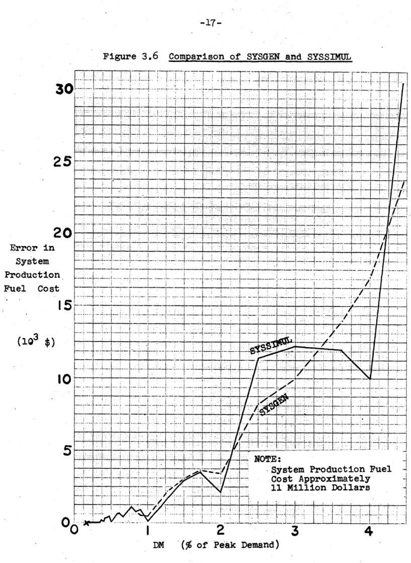
3.3 Comparison of SYSGEN and SYSSIMUL

In order to test the purely numerical round-off differences between SYSGEN and an MIT-corrected version of SYSSIMUL, a

typical one month period with a 9000 Mw peak was repeated, varying only the spacing DM (the size in Mw of the equivalent load

steps). All valve points were chosen as multiples of 30 Mw so that DM = 30 yielded a numerically exact solution.

The following conclusions were drawn firom the comparison: (1) Both codes show error harmonics at factors of 2% of the

peak. (See Figure 3.6). This is due to the fact that two sources contribute to the errors. The first is

101"- 1 F 51U. 1024- 2 F b4.U 201i- I F 680. 2023- 2 F 100. 203: - 3 F 3b09 3OIL- I F 34+0. 302.-- 2 F 1460. 303u- 3 F 1750. 401- 1 F 2:50. 402J- 2 F 4?J. 1501 t- 1. F 500. 502c- 2 F 700. 503.- 3 F 1130. 601r- 1 F 69o. 602'- 2 F 2boo. 603r: 3 F en20. 701X.- I F f3o0. 7026- 2 F 4200. 801m- 1 F 4160. 9R2mi 2 F 5980. No MLIZED SUSD AA .02 .09 .69 e4 04 .02 - LOAD tYPES 6 .9955 .7105 .415; .9810 .675 .3795 .67 5 10 26800 '45 12500 65 13420 90 13700 100 14540 .94 5 3s 12610 40 10790 55 11130 75 11160 120 12120 .90 4 30 12760 70 10640 110 12180 120 13400 .'0 5 3Q 12770 80 10500 100 14100 110 1135t0 120 11950 4 5 380 19550 120 11610 ol435 e10 40 106 0 78 1988 0 12480 .09 4 60 9450 180 8020 210 d260 220 870 .81 5 140 9q70 180 7'A90 260 t120 310 b460 320 8860 .o6 4 30 12380 90 9860 120 10140 140 11340 .92 5 35 13360 11 8750 145 9230 15, 9400 160 9850 .94 5 30 13190 75 9080 100 120 125 9350 140 95j0 .94 5 45 11040 80 7950 3 0 6410 150 8610 160 87 0 .90 5 45 11030 75 8260 15 8430 150 8480 Ib 9590 .91 S 25 13220 90 9470 10 10040 135 10610 160 11560

.o7 5 100 9o40 130 8490 260 6540 29o0 8660 320 8920

.92, 6550 1 00 10410 140 Q0.408600 5j 7118 218Q .7998 3158f 95 60 288796 .95 0 0 400 37 .od 5 200 10 20 400 6600 540 9090 970 9510 600 9670 .87 5 200 9760 390 7930 530 d270 580 bb60 600 8740 9 5 270 9660 450 7940 650- 6310 750 8510 800 8710 .4 .56 .70 .79 .85 .89 .76 .64 .50 .32 .16 .08 .9565 .642 .348 .9235 .6045 .3145 .8835 .5715 .27--b .1335 .1105 .0655 585 4 .3 .0 PRINT MIDI

T;. 5 IS A SAMPLE SYSGEN RUN FOR ONE PLRIOD

50nn - 1i0 720 15 .8325 .5295 .2335 . 27 7 ; .787 .4835 .1960 . 135 50 n .7505 .4505 .1625 . 7 SUSD DATA 9 6 -0 203 3032 02 502 602 606 701 102 801 802 63 3 8 8 3 0b-1 303 8u1 802 50-- 303 60U 60 802 602 701 702 50-2 08 60 8 801 402 603 502 602 303 302 30t 302 302 503 503 503 503 501 6 701 702 501 501 402 202 203 501 203 402 401 601 301 701 702 5 ?O3 _0e 503 _10R 201 ₁₀₄ 701 _{02 41} Z82, 402 11 401 _{b0 042?} T01 401. 202 61 301 _{20 0}

₀₀

PROPOSED FOSSIL PLANTS TO BE USED IN SENSITIVITY STUDY (SECTION 3.6) MAINI. DATA ?01 21 4 14 202 22 5 15 203 23 6 10 301 31 7 17 302 32 8 16 19 303 33 11 27 401 41 9 24 402 42 14 34 501 51 15 35 601 61 17 3n 602 62 27 51 .03 3 2Z37 .7 272 5 -801 81 21 45-802 82 15 45-COmPJTE S AVr

UUTPJT PRINT MINI COMPJTE

STOP

01

0*1

PLANT DATA FOR 20 STATIONS

INDEX IDNO NAME MAXAW

1 2 3 4 5 6 7 8' 9 10 11 12 L3 14 15 16 17 18 19 20 101 102 201 202 203 301 302 303 -401 402 50-1, 502 503 601 602 603 701 702 801 802 A- B- 8- C- D- E- F- G- H-1 2 1 2 3 1 2 3 1 2 1. 2 3 .1 2 3 1 2 .1 2 100 120 120 120 120 120 220 320 140 160 140 160 160 160 320 320 600 600 600 800

TYPE SUSDHT(MEGABTU) PNOM NPTS MWPF(I,INDEX),HTRAT(IINDEX),I=1,NPTS MWPT IN MW & HTRAT IN BTU/KWH

F F F F ~ F F F F F F F F F F F F F F F F 510.00 640.00 850.00 1050.00 .360.00 340.10 1460.06 1750.00 250.0O 420.00 500.00 700.00 1130.00 690.00 2600.00 2820.00 3360.00 3200.00 4160.00 5980.00 0.87000 ~0.943000 0.90.030. C. .93000 0.*85000 0.91000 C. 89000 0.87000 0.85000 0.92000 0.94000 0.94000 0.90000 0.91000 0.87000 0.92000 0.85000 0.88000 0.8700.0 0.89000 10 35 30 30 35 35 60 140 30 35 30 45 45 25 100 100 200 200 200 -270 26800. 12810. 12780. 12770.-11620. 12410. 9450. 9670. 12380. 13360. 13190. 11040. 11030. 13220. 9840. 10410. 10320. 10320. 9760. 9860. 45 40 70 80 80 40 180. 180 90 115 75 80 75 90 .130 140 400 400 390 450 125C 01 10790. 10640. 10500. 9310. 10620. 8020. 7890. 9860. 8750. 7950. 8260. 94-70. 8490. 7110. -8600. 8600. 7930. 7940. 65 55 110 100 90 70 210 280 120 145 100 130 115 110 260 210 530. 530 53C 650. 13420. 11130. 12180. 11100. 9380. Ic980. 8260. 8120. 10140. 9230. 9120. 8410. 8430. 10040. 8540. 7990. 9050. 9050. 8270. 8310. 90 75 120 110 105 120 220 310 140 155. 125 150 150 135 290 305 570 570 580 750 13700. 11180. 13400. 11350. 9550. 12480. 8570. 8460. 11340. 9400. 9350. 8610. 8480. 10610. 863-0. 8470. 9510. 9510. 8680. 8510. 100 14540. 120 12120. 120 1195*. 120 11610. 320 8883. 160 9850. 140 9520. 160 8750. 160 9590. 160 11560. 320 8920. 320 8750. 600 9670.. 600 9670. 600 8740. 800 8710.

MAINTENANCE STRATEGY BY PERIOD AND INDEX (0=NON-EXISTENT;1=DOWN;2=N-LINE)

1NDEX IDNO 101 102 201 202 203 301 302 303 401 402 501 502 503 601 602 603 701 702 801 802 1 2 3 4 PERIOD 5 20000 20000 20000 20000 20000 20L00 20000 20000 20000 20000 20COO 2C000 20000 20000 20000 20030 20000 20000 20000 20000 6 7

- NORMALIZED STARTUP & SHUTDOWN FUNCTICN :

0.09,J00 0.340000- 0.56060 0.700000 9.79C000U 0.a40000 0.760000. 0.640C00 0.500000 0.3200300 0.020000 0.010000 0.0 0.85000 0.890000 C.160000 0.080000 1 2 3 4 '.5 6 7 8 9 10 11 12 13 14 15 16 17 18 19 20 8 9 1 0 I, 0.0200 00 -0.890000 0. C4( 0CC Figure 3,3

STRATEGY 10 = PERIOD NUMBER = PKMW 50C0.00 1* 1

TITLE :"PROPOSED FOSSIL PLANTS TO BE USED IN SENSITIVITY STUDY (SECTION 3,6) "

TITLE :"1THIS IS A SAMPLE SYSGEN RUN FOR ONE PERIOD

OT(HRS) 720.00. LDTYPE I DM= 100.0000 PROB K) ,K=1,EMAX 1 .0c3000000 1.000000000 1.ooooooo O 1.00000oco 0.883500000 0.832500000 0.483500000 0.450500000 0.133500000 0.110500000 0.0 IEMAK = 51 1.000000000 1.0000000.0 0.787000000 0.415000000 0.085500000 1.000000000 1.010000000 0.75050V0000 0.379500000 0.058500000 PEMAX . 5100.0010 1 .000000000 1.000000000 0.710500000 0. 348000000 0.041500000 1.000000000 1.000000000 0.675000000 0.314500000 0.027000000 1.000000000 0.995500000 0.642)000000 0.275000000 0.013500000 1.003000000 0.981000000 0. 6045)0000 0.23350000 .0.007000003 1.000000000 0.956500000 0.571500000 0,196000300 0.0030C.0000 1.00000.0 CO 0.923500000 0.529500000 0.16250000, 0.0

COST OF EMERGENCY POWER = 7.5000 $/MWH

INDEX IDNO NAME MAXMW TYPE STAT.AVLBTY CSTBTU SUPCST ENERGY NPTS (MWPTMRGCST) IN UNITS OF (MW,$/MWH)

1 2 3 4 .5 - 6 7 8 9 10 11 12 '13 14 15 16* 17 18 19 20 101 102 201 202 203 301 302 303. 401 402 501 502. 503 601 602 603 701 702 801 802 A- B- C- D- E- F- E- F- G- H-1 2 3 1 2 3 I 2 3 2 2 3 1 2 3 1 2 1 2 100 120 120 120 120 120 220 320 140 160 140 160. 160 160 320-320 600 600 600 800 F F F. F F F F F F F F F F F F F F F F F LOADING ORDER BY (1000*NP 1002 3012 3007 1006 3004 1005 1008 4008 4016 4007 1013 4017 4018 3002 4002 1010 1012 2015 4020 2013 3013 5011 4005 4004 4009 87.000 94,000 90.000. 90.000 85.000 91.000. 89.000 87.000 85.000 92.OCO 94.000. 94.000 90. 000 91.000 8 7. 000 92.000 85.000. 88.000 87.000 89.000 50.0-00 50.000 50.000 50.000. 50.000 50.000 50.000 50.000 50.000 50.000 50.000 50.C000 50.000 5C.0 00 50.000 50.000 50.000 50.0003 50.000 50.000 255. 320. 425. 525. 180. 170. 730. 875. 125. 210. 250. 350. 565. 345. 1300. 1410. 1680. 1600. 2080., 2990. 0.0 0.0 c.0 0.0 090 0.0 0.0 0.0 0.0 0.0 C.0 0.0 0.) 0.0 0.0 C.3) 0.0 C.0 0.0 0.0 5 5 4 5 5 4 -4 5 4 5 5 5 5 5 5 5 5 5 5 5

T + INDEX) I.E., NORDER(I),[=1,NNORD

1015 1016 1017 1018 1019 1020 2016 200j 3015 2017 2018 4012 4019 4015 5C2) 501 4013 1011 1014 3017 3018 2011 3C11 301 10 35 30 3a 35 35 60 140 30 35 30 45 45 25 100 1 OC 200 200 200 270 13.400 6.405 6.390 -6.385 5.810 6.205-4.725 4.835 6.190 6.680 6.595 5.520 5.515 6.610 4.920 5.205 .5.160 5.160 4.880 4.930 45 .40 70 80 80 40 180 180 90 115 75 80 75-90 130 140 400 400 390 450 WITH NNORD = 96 B 2019 2020 9 2010'5016 ) 1004*2005 6 .250 5.395 5.320. 5.250 4.65.5 5.310 4.010 3.945 4.93) 4.375 4.540 3.975 4.130 4.735-4.245 3.555 4.300 4.303 3.965 3.970 2U12 3016 3008 5012 5015 5008 4011 3005 4010 5013 1003 5017 5018 5010 1001 2009 3014 3009 2004 4014 2006 2003 5014 5005 5004 5002 3003 '4006 2001 4003 3001 4001 5001 65 55 110 100 90 70' 210 280 120. 145' 100 130 115 110 260 210 530 530 530 650 3019 1007 1009 2002 6.710 90 5.565 75 6.090 120 5.55) 110. 4.690 105 5.490 120, 4.130 220 4.060 310 5.070 140 4.615 155 4.560 125 4.205 -150 4.215 150 5.020 135 4.270 290 3.995 305 4.525 570 .4.525 570 4.135 580 4..155 750 6.853) 5.590 6.700 5.675 4.775 6.240 4.285 4.230 5.670 4.700 4.675 4.305 4.240. 5.305 4.340 4.235 4.755 4.755 4.340 4.255 100 7.270 120 6.060 ******** *** 120 5.975 120 5.805 320 4.440 * ** ******* 160 140 160 160 160 320 .320 600 600 600 800 4.925 4.760 4.375 4.795 5.780 4.46) 4.375 4.835 4.835 4.370 4.355 3020 2007 2014. 3006 / INDEX I F-J 1 2 3 4 .5 6 7 8 9 10 11 12 13 14 15 16 17 18 19 20

PERIOD NUMBER = 1 TITLE :"THIS IS A SAMPLE SYSGEN RUN FOR ONE PERIOD INDEX ID I 1' 2 1 3 2 4 2 5 2 6 3 7 3 8 3 9 4 10 4 11 5 12 5 13 5 14 6 15. 6 16 6 17 7 18. 7 19 8 20 8 NO 01 02 01 02 Q3 01 02 03 01 02 01 0~2 03 01 02 03 01 02 01 02 NAME LD FACT A- B- C- D- E- F- G- H-Ha 1 2 1 2 3 1 2 3 1 2 1 2 3 1 2 3 2 1 2 0.047136 0.321493 0.081873 0.116620 0.359161 0.091880 0.404130 0.833049 0.111392 0.501317 0.250933 0.817176 0.340752 0.159768 0.682332 0.844545 0.545903 0.539992 0.810960 0.809516 OPER HRS 82.4256 676.8000 96.0441 156.6045 612.0000 119.9870 309.5443 626.4000 127.4397 662.4000 247.9156 676.8000 267.9585 233.9119 626.4000 662.4000 612.0000 633.6000 626.4000 640.8000

STARTUPS & SHUTDOWNS

NUMBER MEGABTU COST($)

7..4379 0. 00 9.9324 20.3006 0.0000 14.5732 25.7082 0.0000 17.4917 0.0000 25.8913 0.0000 26.7000 25.6682 0.0000 0.0000 0.0000 0.0000 0.0000 0.0000 3793. 1897. 0. 4221. 10658. 0. 2477. 18767. 0. 2186. 0. 6473. 0. 15086. 8856. 0., 0. 0. 0. 0. 0. 0. 8443. 21316. 0. 4955. 37534. 0. 4373. 0. 12946. 0. 30171. 1-7711. 0. 0. 0. 0. 0. 0. EXPECTED PRODUCTION ELECT(GWH) 3.39379 27.77701 7.07381 10.07594 31.03149 7.93843 64.01421 191.93450 11.22829 57.75169 25.29401 94.13866 39.25459 18.40529 157.20931 194.58318 235.83003 233.27653 350.33484 466.28122 MEGARTU' COST($) ,28030. 1754CY2. 42277. 59063. 170106. 47822. 271683.. 848129. 61098. 307973. 131059. 431891. 181245.. 100644. 714095. 860059. 1127653. 1120027. 1526820. 2058441.. 56061. 350803. 84554. 118127. 340211. 95645. 543366. 1696258. 122196. 615946. 262118. 863782. 362490. 201287. 1428190. 1720117.-2255307. 2240055. 3053641. 4116882. TOTALS

MEGABTU COST($) INDEX

59854. 350803. 92996. 139442.. 340211. 1.00600. 580900. 1696258. 126569. 615946. 275064. 863782. 392661. 218999. 1428190.. 1720117. 2255307. 2240055. 3053641. 4 116882. 29927. 175402. -46498. 69721. 170106. 50300. 290450. 848129. 63284. 307973. 137532. 431891. 196331. 109499. 714095. 860059. 1127653. 1120027. 1526323. 2058441. 1 2 3 4 5 6 7 8 9 1) 11 12 13 14-15 16 17 18 19 20 P O W E R INSTALLED ON-LINE PEAK LOAD CAPACITY CAPACITY FORECAST

LOSS-OF-LOAD PROBABIL ITY

E N E R G Y:

EXPECTED DEMAND EXPECTED PRODUCTION EXPECTED EMERG PURCH

(UNSERVED BY DIRECT CALC

C 0 S T:

PRODUCTION FUEL

STARTUPS & SHUTDOWNS EMERG.PURCH.@ 7.500 $/MWH TOTAL MEGAWATTS 5400 5400 5000 0.041888 GWH 2237.8320 2226.8268 11.0052 .11.1447) DCLLARS 10 263517.-70621. 82539. 10416677. H a-' Figure 3.5 SYSGEN Period Output

Figure

3.6

30

2.0

O

(103

$)

10

hit

System Production Fuel

Cost Approximately 11 Million Dollars

DM2

3

4

code attempts to represent varying plant sizes as multiples of a single step size, DM. The first error obviously goes to zero at steps that are factors of

2% (e.g., 0.5, 0.67, 1.0%) while the second error continues to grow as DM increases.

(2) SYSGEN gives much smoother behavior with increasing step size (Again, see Figure 3.6).

(3) SYSGEN is about four times faster than SYSSIMUL and (4) Steps on the order of 1 to 2% of the peak provide

consistent. results in reasonable amounts of computer time. (A system containing 70 plants can be simulated by SYSGEN over a single time period in under 3 seconds on an IBM 360/65 computer).

3.4 Optimization Model

For the sake of completeness in explaining the optimization scheme, the system integration model will first be restated

(See Figure 3.1).

Taking due account of initial conditions and various

re-fueling and maintenance constraints, the Rere-fueling and Maintenance model determines feasible sets of nuclear refueling dates and

associated fossil maintenance schedules that are stored as "Possible Alternatives" to be investigated further.

Choosing these alternatives one at a time, the 5 to 10

year horizon of the multi-year study is divided into equal periods (on the order of 1 to 4 weeks) during which the availability,

of production is done for each of these time periods using the Booth-Baleriaux model.

The startup order used in the model is arrived at by

noting two important points. First, on a time scale where fuel is being designed, nuclear units are not energy-limited.

Therefore, nuclear production should not be scheduled as a scarce resource. Secondly, since the best-plant fossil

incremental costs are presently higher than even the highest nuclear average costs, nuclear power should be operated so as

to displace maximum fossil energy. Thus, after starting up

and raising to minimum power those fossil plants that will not be shut down, all nuclear plants are started up and loaded to full power. Finally, all the remaining fossil power is utilized

in order of increasing incremental cost.

The output of the model at this stage is minimum fossil total cost and maximum expected system nuclear energy ("nuclear potential") that is to be generated in each period to meet the given loads. Repetitive use of the Booth-Baleriaux model for each time period of the study has thus separated the fossil and nuclear portions of the system. Now the optimization task is to meet the resulting nuclear potential at minimum cost. In other words, now it is strictly nuclear marginal cost versus nuclear marginal cost to determine which nuclear plant generates which portion of the nuclear potential.

Still referring to Figure 3.1, nuclear optimization begins by utilizing the initial fuel cost estimates to schedule

model. These production requirements are then passed to the Core Simulation and Optimization model which designs the fuel reload batches (batch size and enrichment) to meet the production schedule and refueling dates at minimum cost. Information

returned to the System Integration and Optimization model is just minimum total system nuclear fuel cost (for later summation

of total costs) and the pertinent nuclear marginal cost of each reload batch. Nuclear production is then tentatively rescheduled so that all nuclear plant reload batches are designed at the same marginal cost. A convergence check is made to determine if the new production schedule differs "significantly" from the previous

one. If it does differ, a feasibility check must then be made to determine if the new schedule can physically be carried out to meet the nuclear potentials. An infeasible schedule is

discarded and another new schedule tentatively proposed, while a feasible schedule is again passed to the Core Simulation and Optimization model for the next iteration in the design.

When such a rescheduling produces no "significant" changes in the production schedule, overall system-core operation has been optimized for the particular "Possible Alternative"

maintenance schedule chosen. Total nuclear and total fossil costs are then added to give total system cost for that alternative.

When all the "Possible Alternatives" have been so investigated, the one resulting in minimum total system cost is chosen.

1_{Network Programming (NP) is a specialized case of linear}

programming which leads to large savings in both computer storage and execution time.

A single NP model will be used for both the initial produc-tion schedule and the feasibility checks. A three reactor-24 period example of the proposed network configuration is shown in Figure 3.7. Numbers are shown for the nuclear

potential to emphasize that this is the fixed constraint through-out one Possible Alternative. The notation E in the bottom row represents energy produced by the r th nuclear plant between the two refuelings representing the i th cycle (i.e., refueling interval). For example, Plant 1 generates an amount of energy E from Cycle 1 until it is refueled in Period 14; then Cycle 2 begins leading to an ultimate energy production by Plant 1 of

E before the next refueling in Period 24. Note that the sum 1,2

of any column must equal the energy extracted during that particular reactor-cycle. Note also that for this three plant example,

the sum across any row represents at most three plants contributing energy such that the total production equals the nuclear potential for that period.

This network configuration is essential to determining if generation can be shifted from one reactor-cycle to another. For example, can E2,3 be increased by A and E3,1 be decreased by A and still meet the nuclear potential constraints?

3.5 Compatibility

As implied in the previous section, the System Integration and Optimization model will be designed to be compatible

with core simulation and optimization modules whose only

requirement is to take a given set of E's and T's (i.e., energies and cycle lengths) and return two specific types of information:

Figure 3.7 Sample Network Configturation

Reactor Reactor 2 eactor 3 Nuclear Period Cycle: Oycle Cyc

1 2 1 2 3 2 Potential --- ---2020 Gwh 2 ₁₉₄₀ 3 1336 4 1828 5 94< 6 2020 7 2071 8 2020

9

2020

1940

18

1

(1) the minimum total system nuclear fuel cost and

(2) a set of nuclear marginal costs for each reactor reload batch (partial derivative of (1) with respect to

each E ).

r!

Note that with the multi-year model of Figure 3.1, specific

information about the fuel designs is not needed by the System

Integration and Optimization model. It doesn't even matter whether the reactors are PWR's, BWR's, HTGR's or fast breeders.

All that is needed by the system optimizer are minimum total

cost and marginal costs. (Of course., management personnel

need fuel design information and it should therefore be available in the computer output from the Core Simulation and Optimization

model).

No absolute dependence on any other work here at MIT will be required. The idea is to make the modules easily hooked together like the boxcars of a train, not nailed together like the track.

To ensure this compatibility and permit concentration on the development of the System Integration and Optimization model, an unsophisticated fuel cost simulator (Figure 3.8)

based on purely empirical relationships will be used to temporarily complete the nuclear power management multi-year model. For

example, no on-line depletion runs will be made, just an adjustable polynomial giving unit fuel purchase cost or

salvage value as a function of initial enrichment and burnup. Reload batch fuel cost will then be calculated using the simple,

Core Simulation and Optimization

Model

REPLACED BY.

Nue1

Initial Conditiont Nuclear Fuel Cost

Data Core Simulation, to Optimize Nucle]a Fukel Design Optimum Reload Fuel: Enrichment Batch Size Mil.Tot .Coat Marginal Coots

f

Data Fiuel Cost Simulator Total Nuclear Fuel Cost Marginal Cost of Each Reload Batch

Compatibility of the Fuel Cost Simulator

1>

Batch Revenue Requirement Batch Initial

Present Valued to Investment

J

(

- Salvagee 1 - y(t"+ ) (3.1)

Value

where y = average cost of money, before taxes t total in-core time

= pre-irradiation payment date t= post-irradiation receipt date

All batches will then be present-valued to the study's base date to yield total nuclear fuel cost. The partial derivative of this total with respect to each E gives the pertinent marginal

costs.

As other fuel cost simulators are developed and evaluated, they can, and will, be used in place of this temporary cost model to supply the System Integration and Optimization model with its required information.

Several reasons preclude immediate utilization of any core simulation or cost calculation modules already developed here at MIT or by the Joint System Analysis Task Force:

(1) avoidance of delays inherent in linking the input/output of the various modules,

(2) verification of the Booth-Baleriaux-Network Programming approach to the problem would be greatly hindered if any problems were -encountered in the work of others,

(3) program size and speed would suffer if a more

sophisticated core simulation or fuel costing code were used in this early experimental phase of

development, and

(4) a "completed package" appeal ought to be avoided in order to encourage others to fill any gaps with their own models and to emphasize areas of development

substantially completed.

Furthermore, in the long term the temporary simulator may be good enough to allow subsequent work merely to

calibrate the constants in the model. In any case, the System Integration and Optimization model itself will not be

invalidated as other simulation and costing models are developed.

3.6 Sensitivity Study

With the nuclear power management multi-year model loop completed (albeit in an ad hoc sense), a sensitivity study will be undertaken to investigate model behavior with respect to

fuel costs, startup costs, cycle lengths and, in particular, replacement energy cost incurred during refuelings. The

tentatively proposed hypothetical utility system will consist of about 20 fossil plants (Figure 3.3), 5 nuclear plants and 15 peaking plants with a capacity mix similar to the Commonwealth system in the late 1970's. Normalized load-duration curves also typical of the Commonwealth system will be used. An 8 year

(96 month) horizon will be studied under 10 to 20 strategies.

Such a study will be useful in pinpointing important research areas and accelerating model improvement. Beyond this, it is

hoped that several operating "rules-of-thumb" can be deduced which, though not perfect for all circumstances, might result in near-optimal decisions.

4.0 THE NUCLEAR IN-CORE SIMULATOR AND OPTIMIZER (J. P. KEARNEY)

4.1 Introduction

It was initially the objective of this part of the over-all study (which will form the basis for Joseph Kearney's the-sis (2)) to perform both the necessary sensitivity studies on nuclear refueling scheduling options and develop the nuclear in-core simulator to be used by the entire system integration and optimization model. As time proceeded, however, it

be-came increasingly obVious that attempting to achieve both goals would require the resolution of two distinct problems. Namely,

the development of the rapid nuclear computer models to be used in a simulation is an entirely different task from that of developing the more accurate nuclear models to be used in in-core sensitivity studies. As a result, it was decided that Kearney would concentrate on the former problem -- development of a nuclear in-core simulator to be used in the MIT utility simulation model. In this way an entire simulation model could be in operation at an earlier date in order to ascertain its operating characteristics. The sensitivity analysis, which will provide very valuable information to the simulator, will be carried out by Terrence Reick (3).

The areas numbered 5, 6, 7 and 8 on Figure 1.1, Nuclear Power Management Multi-Year Model, display the function this simulator and optimizer plays in the overall system simula-tion. This problem is to choose for each reactor the correct,

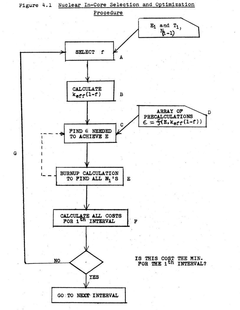
i.e. minimum cost, method of producing the required. amounts of energy in the time intervals specified by the system inte-gration and optimization model; see Section 3 of this report. The in-core simulation and optimization problem is out-lined in more detail in Figure 4.1. In short, a schedule of E _ri 's and T _r,i's, the energy and time in each refueling

in-terval, i, for each reactor, r, is generated by the system simulator. The nuclear in-core simulator and optimizer must find the schedule of e 's the enrichment of the fuel to be

fed into each reactor at the beginning of refueling interval i, and f r'a, the fraction of the core into which fresh fuel

will be placed at the beginning of refueling interval i, that minimizes the cost of electricity from that nuclear plant

over the entire planning horizon of about five years.

The scope of this work will be described in three por-tions. First a nuclear in-core model that would adequately describe the neutronic and material characteristics of nuclear fuel as a function of time has to be developed' Block E on Figure 4.1. The majority of work on the in-core simulator and optimizer has been carried out in this area since Pro-ject Report No. 1 of January 1971 (1). The second portion of the task is to develop a method of selecting the refuel enrichment required to produce a specified amount of elec-tricity, Er, assuming the refuel fraction is known. Block C in Figure 4.1 indicates where this function is performed

Figure 4.1 Nuclear In-Core Selection and Optimization Procedure A B

ARRAY

CALCU E ALL COSTS

FOR i VuINTERVAL

IS THIS COST THE MIN. FOR THE ith INTERVAL?

G

A) arbitrarily from a set of feasible f's and with the use of a set of precalculations (Block D) the enrichment re-quired to produce Z. is odnd. This-procedure _{will be} de-scribed in Section 4.3. The third area of concern is in developing an optimization procedure to find the set of E

and f 'sthat satisfy Ei and T at minimum cost. Very sim-plistically, this procedure is indicated by the feedback loop

designated G in Figure 4.1.

4.2 The MOVE Code

As was mentioned, the work to date has been concentrated in the area of selecting a nuclear in-core model. The charac-teristics of any computer code to be used in this capacity are that it must be fast, sufficiently accurate, and flexi-ble, since it will be required to handle many different com-binations of enrichments and refuel batch fractions at each refueling. Simplified input is a requirement for the same

reason.

A mesh point sensitivity analysis was carried out using the MOVE code (8) and the San Onofre reactor as a model. Table 4.1 presents the results of this study. Assuming that the discharge burnup of 33,450 MWD/T given by Combustion Engi-neering (9) for the San Onofre reactor utilized a more accu-rate calculational technique than we have available to us, this value was used as a basis for comparison as the number of mesh points was varied. Note that there is no

signifi-Table 4.1

Sensitivity of MOVE to Number of Mesh Points*

Steady State Cycle (3.3 w/o = e) = 33,450) Number of Mesh Points 270 [18x15] 144 [18x8] 100

ClOx10]

e CPU Time Deviation in E [mils/kwhr] [min/cycle] [%] 1.8531 1.8432 1.8492 1.8446 1.20 0.83 0.55 0.44 1.56 2.28 1.51 1.90 *San Onofre Reactors 2 and 3 (9)

cant loss of accuracy as the number of mesh points decrease, but there is a large savings in computer time. This

demon-strates that the MOVE code satisfies the first two characteris-tics mentioned above, speed and sufficient accuracy. There-fore, the MOVE code with the 10 x 8 mesh point arrangement will be used as the in-core simulator.

Table 4.2 is a tabulation of the MOVE and FLARE results for the Zion reactor from initial core loading to steady state operation. Note the very minimal differences in all of the burnups for the Zion reactor. More importantly (notes 1 and 2 in Table 4.2) observe the savings to be gained by using the MOVE code. This savings can be further increased by decreas-ing the number of mesh points used in MOVE. As was previously shown going to a 10 x 8 mesh point arrangement does not sig-nificantly effect the accuracy of MOVE. This is even further substantiated in Table 4.3 where the Zion results for this and a 15 x 15 mesh point arrangement are tabulated.

The third characteristic that any in-core simulator that is to be used in an optimization procedure must have is flexi-bility. The simulator must be able to consider any number of refuel enrichments automatically and must be able to refuel with any specified batch size. The MOVE code has been

modi-fied to consider fuel of differing initial enrichments. It can store the necessary CELL code information for five dif-ferent enrichments and can at the command of the operator place variously enriched fuel into any zone in the reactor.

Table 4.2

Comparison of MOVE and FLARE3 _{Results for Zion Reactor} Approach to Steady State

Initial Core Enrichments 2.25, 2.8 and 3.30 w/o Refueling Enrichment 3.2 w/o

Cycle No . 1 2 3 4 5 6 7 8 9

Average Discharge Burnup, MWD/T MOVE1 14,906 25,050 30,173 29,766 29,901 29,896. 29,896 29,896 29,896 FLARE2 14,980 24,812 30,014 29,286 29,422 29,340 29,616 29,486 29,548

Core Average Burnup MWD/T MOVE1 15 ,073 8,668 10,044 10,038 9,933 9,965 9,965 9,965 9,965 FLARE2 12,950 10,200 9,719 9,360 9,799 9,798 9,800 9,849 9,852

1) Preparatory CELL run - IBM 360/65 First 6 cycles with MOVE

Total 2) Preparatory LEOPARD and PDQ-5 runs

-IBM 360/65

First 6 cycles with FLARE

Total $9.00 34.00 $43.00 $153.00 102.00 $255.00 MIT IBM 360/65 cost $1.90/minute at low priority.

Table 4.3

Sensitivity of Zion Results to the Number of Mesh Points for MOVE

Zion PWR Approach to Steady State Initial Core Enrichments

Refueling Enrichment 2.25, 2.80, 3.3 w/o3.2 w/o

Cycle No. 1 2

3

Average Discharge Burnup [15x15] Meshi [1Ox8] Mesh2

14,906 25,050 30,173 29,766 29,901 29,896 15,427 25,182 30,828 29,190 29,396 29,368

1) Cost for first six cycles on IBM 360/ $1.90/minute

Average Core Burnup

[15xl5] Mesh [10x8] Mesh 15,023 15,896 8,668 8,881 10,044 9,787 10,038 9,893 9,933 9,749 9,965 9,794 65 $34.00

2) Cost for first six cycles on IBM 360/65

Furthermore, it can now select any one of these enrichments to be used for the fresh fuel at each refueling, or the

opera-tor could specify a long series of refuel enrichments to be used automatically by the code at each refueling.

During the optimization procedure the in-core simulator will be used many times. Each time the simulator is called

the results it generates will be transferred out of the MOVE code and stored, see Figure 4.5. Due to this transferring

and storing, the information that characterizes-the state of

the reactor must be kept to a minimum in order to conserve computer storage space and computer time. In the case of the MOVE code there are only three pieces of data that need be preserved to completely describe the state of the reactor at

any time. These are the number of zones in the reactor, the initial enrichment associated with each zone and the burnup of the fuel at each mesh point.

4.3 The Proper Selection of Refuel Enrichments

The second major area of concern in the development of a nuclear in-core simulator and optimizer will be the selec-tion of refuel enrichment given the refuel batch size and the required energy output for the reactor during the next refueling interval, Blocks B, C and D of Figure 4.1. As indicated in Figure 4.1, a set of precalculations will be

made which will describe the relationship between refuel batch size, enrichment and required energy production. Basically,

deriving this relationship depends upon finding an adequate index of the reactivity, or energy producing capacity, re-maining in the core after a fraction, f, of the core has been removed. The complication arises in that the energy pro-duced in the remainder of the core, (1-f), during the next refueling interval will depend on the refuel enrichment, be-cause the flux experienced by the inner region (the (1-f) region) of the core is very dependent on the enrichment of

the outer region, the new fuel region. Consequently some account must be made for the flux shape in the (1-f) region of the core if the index is to be an accurate measure of the energy producing capacity in that region. As indicated in Figure 4.2,Block B, the first index which shall be tested is keff of the remainder, (1-f), region of the core. This work is commencing now using the MOVE code and the Zion reac-tor.

4.4 The Optimization Procedure 4.4.1 Introduction

There are three characteristics of any optimization

procedure selected for use in finding the minimum cost scheme for refueling the reactors in a utility system. It must (1) be successful, i.e. it must find the optimum scheme, (2) elimi-nate some alternatives as it proceeds -- an exhaustive search of all alternatives is not acceptable in this case, and (3)

be flexible. With respect to flexibility the optimization technique selected must have the facility to accept new in-formation which might radically change the procedure as more information about utility system simulation is generated. Typically as refueling scheduling sensitivity studies (3)

begin to generate information, it must be incorporated into this optimization. Furthermore, when a method for evalua-ting the worth of reactor fuel at any point in time is de-rived (4) the optimization procedure is simplified tremen-dously, and the procedure selected now must have the flexi-bility to optimize using this information later.

4.4.2 The Nature of the Problem

The nature of the optimization problem can be described using Figures 4.2, 4.3, and 4.4. For the reactor in question a schedule of E r,i's and T 's is given. Furthermore, the material densities, N i's, of the fuel at the beginning of the planning period are given. This is shown'in Figure 4.2, Input Variables to the Optimizer, for a five interval plan-ning period. Each refueling interval is the time period be-tween the start of two fuelings.

For a reactor, whose state is defined by the spatial distribution of nuclide concentrations, the selection of a reload batch fraction f uniquely defines the reload enrich-ment required to produce the energy Er'i during the next

fueling interval. Therefore, f was chosen as the variable to optimize.

OPTIMIZING f GIVEN N (i) S Er,l Tr 1 Interval 1. Er,2 r., 2 2. Figure 4.2 0.4 0.3 0.2 0.1

Input Variables to the Optimizer

t EACH Ci IS MINIMIZED.

5

BUT E C IS NOT MINIMIZED!

5

MUST WE CALCULATE E C FOR ALL POSSIBLE PATHS? ial

Figure 4.3 A Typical Optimized Path of' f's Er 3 Tr.,

3

1. 2. 3. if 0.3 0.2 if 0.3 0.2

Total No. of Paths = 4

1. 2. 3.

INTERVAL STEP III

Total No. of Paths = 8

Figure 4.4 Nuclear Fuel Management Decision Tree INTERVAL

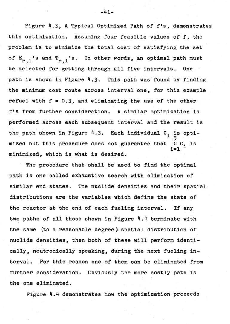
Figure 4.3, A Typical Optimized Path of f's, demonstrates this optimization. Assuming four feasible values of f, the problem is to minimize the total cost of satisfying the set of E r,'s and T 's. In other words, an optimal path must be selected for getting through all five intervals. One path is shown in Figure 4.3. This path was found by finding the minimum cost route across interval one, for this example refuel with f = 0.3, and eliminating the use of the other

f's from further consideration. A similar optimization is performed across each subsequent interval and the result is the path shown in Figure 4.3. Each individual C is

opti-5

mized but this procedure does not guarantee that E C is i=l

minimized, which is what is desired.

The procedure that shall be used to find the optimal path is one called exhaustive search with elimination of similar end states. The nuclide densities and their spatial distributions are the variables which define the state of the reactor at the end of each fueling interval. If any two paths of all those shown in Figure 4.4 terminate with the same (to a reasonable degree) spatial distribution of nuclide densities, then both of these will perform identi-cally, neutronically speaking, during the next fueling in-terval. For this reason one of them can be eliminated from

further consideration. Obviously the more costly path is the one eliminated.