Dynamics and NMR implementation of controlled-NOT gates for quantum computing

Dynamics and NMR Implementation of Controlled-NOT Gates

for Quantum Computing

by

aMy e dunlop

A.B., Chemistry and Physics

Harvard University, March 1996

Submitted to the Department of Nuclear Engineering in Partial Fulfillment of the Requirements for the Degree of

Master of Science in Nuclear Engineering at the

Massachusetts Institute of Technology

June 1998

© 1998 Massachusetts Institute of Technology. All rights reserved.

Signature of Author

aMy

e

dunlop

Department of Nuclear Engineering

18 May 1998 Certified by

0" ' David Cory Associate Professor of Nuclear Engineering

f' Thesis Supervisor Accepted by 14- ' !!VbWW i,

b~':$

1 i

Chairman, Department Committee on Graduate Students

scawe"

-Dynamics and NMR Implementation of Controlled-NOT Gates

for Quantum Computing

by

aMy

e

dunlop

Submitted to the Department of Nuclear Engineering on 18 May 1998 in Partial Fulfillment of the

Requirements for the Degree of Master of Science in Nuclear Engineering

ABSTRACT

NMR experiments implementing two-bit controlled-NOT logic gates on alanine (JAB = 35.1 Hz) and 2,3-dibromothiophene (JAB = 5.6 Hz) were performed. Spectra were collected at a variety of tip angles (angles between the spin and the axis of magnetization) by applying a selective RF pulse of constant power and variable duration. From this collection of spectra, the effective Hamiltonian of the spin system was derived and found to contain an internal Hamiltonian. In a spin system with weak coupling, the internal Hamiltonian contains spin-spin coupling terms. The effective Hamiltonian gives a more complete description than the currently used transition Hamiltonian.

Understanding the dynamics of a spin system not only furthers the field of NMR but has application in the subject of quantum computing. NMR pulse sequences for four-, eight- and 16-spin controlled-NOT logic gates were developed. A pattern is evident and the pulse sequence for any number of spins can be derived. Disregarding the differences in the spin-spin coupling constants of different spin systems, these results suggest that the total time to implement a controlled-NOT logic gate in NMR does not increase exponentially with the number of spins in the system.

Thesis Supervisor: Title:

David Cory

The computational speed of the classic computer is limited by the size of the computer's

components and the speed at which they can be driven. Eventually, computer components will be so small that quantum effects cannot be ignored. A computer that relies on quantum coherence

may permit a future generation of computers to have capabilities that far outreach their classic predecessors, which adhere to the laws of classical physics.

However, a quantum computer of a size greater than six-bits has yet to be built and the physical realization of such a quantum computer is still many years away. These machines will perform reversible, unitary computations on a system including quantum superpositions. The reality of being able to create an efficient, user-friendly two state system with coherence times that are long enough to do multiple computations is a formidable goal. Quantum computing systems are being researched. The ion trap method uses the quantized energy levels of an atom as the states of the bit [Cirac95]. Computations are performed using lasers to impart detectable energy and momentum to the system. An extension of the ion trapping idea uses high-Q optical cavities to transfer information between ions and the field modes. If realized, this will be the first example of quantum information transfer [Davidovich94].

Another family of paradigms uses a coupled system of spin = % particles. Spin up and spin down provide an easy analogue of the classical binary states. Nuclear spins are preferred over electron spins because the smaller magnetic moment of the proton means a weaker dipolar magnetic interaction and a much longer time period of coherence. Because standard techniques have already been developed and spin systems can be put into pseudo-pure states that evolve under a well-studied Hamiltonian, NMR (nuclear magnetic resonance) has been a fairly successful method of implementing unitary, reversible quantum computations [Cory96], [Cory97],

[Gershenfeld97], [Lloyd93].

In NMR quantum computing, each molecule acts as a separate quantum computer and the number of resolvable spins in the molecule determines the number of bits in the computer. The nuclear spins are quantized in a magnetic field and a computation is performed on the initial spin state by applying a series of RF (radio-frequency) pulses resonant at the frequency of the desired transition. Because each NMR sample has on the order of 1023 molecules, a computation is

massively redundant; each measurement is a measurement of an ensemble of states. While quantum computation relies on the deterministic, measurement of a random state, measurement of an ensemble provides a stochastic average of a large number of random states. [Cory97].

The study of quantum computing, the science of computation using components small enough that their dynamics are governed by the principles of quantum mechanics, is already many years old. In the 1980's, Feynman introduced the idea of using systems governed by quantum mechanics to explore complex quantum phenomena. This exploration of

quantum-based systems led to the idea that other problems could be solved by adhering the rules of quantum mechanics. The possibilities of solving problems once deemed unsolvable or solving

problems with more efficient algorithms, inspired many. Shor proved that using quantum algorithms, computers would be able to factor large numbers in polynomial time as opposed to the exponential time it takes classical computers [Shor94]. Grover developed a quantum

algorithm that searches through a database with N items in an average of /N tries as opposed to the N/2 average associated with classical computer algorithms [Grover96]. Deutsch, DiVincenzo and Barenco have transformed the idea of classical universal gates into quantum complete and quantum universal gates.

With the suggestion that quantum algorithms are sometimes more efficient and in some cases capable of solving computational "hard" problems, the excitement behind the field of quantum computing continues to grow. People are talking about the eventual necessity of

quantum computers to safeguard encrypted data. Physicists are developing quantum techniques with the hope that a system based on quantum principles will provide insight into quantum phenomena. While many people have embraced the idea of quantum computing, the immediate gratification is coming from its secondary results. Implementation of quantum computing ideas, in addition to further advancing the somewhat elusive goal of building a quantum computer, is advancing quantum information theory, laser applications, ion trapping methods, methods of error correction, the understanding of complex quantum phenomena, and the field of NMR.

This paper focuses on the use of NMR to study ideas and algorithms of quantum

computing. Following Chapter One's introductions to NMR and quantum computing logic gates, Chapter Two describes experiments implementing a two-spin controlled-NOT gate with the Pound-Overhauser technique. The chapter contains a discussion of the Hamiltonian associated with the state transition in a two-spin quantum controlled-NOT gate and argues that the standard picture of the transition Hamiltonian is incomplete. Chapter Three discusses multiple-spin controlled-NOT gates and the NMR pulse sequences needed to implement them. The final chapter discusses the impact of this work, future experiments and the NMR paradigm of quantum computing. Though problems exist, research being done to implement today's quantum computing ideas with NMR will be applicable to any paradigm of quantum computing, advance new theories of quantum computing and inspire new ideas in the field of NMR.

Chapter One. Introduction.

Quantum Computing: An Application of NMR.

Basics of NMR. NMR (nuclear magnetic resonance) is a method of spectroscopy first developed in the

1940's. NMR is most commonly used in chemical and structural analysis and also medical imaging. The

sample's nuclear spins are quantized in a magnetic field of several Tesla. The state is governed by the

Zeeman Hamiltonian,

Hzeeman = (-y h Bo) Iz

(1)

RF pulses are used to manipulate the state of the spin. Pulses are designed to induce either all of the transitions allowed by quantum mechanics or a selective set of them. The RF Hamiltonian in a stationary

frame of reference is,

HRF = RF (Ix - ). (2)

The component of the spin magnetization that is put into the transverse plane precesses about the axis of

magnetization. The rate of this precession is governed by T2, the spin-spin relaxation. Because of this

precession, it is useful to use the HRF in a rotating frame,

HRF-rotating

e

+ ) *JAB*time) *

HRF

e(-i

Following the RF pulse, the T1 (spin-lattice) relaxation dictates the return of the spin state to thermal

equilibrium. The relaxation results in a measurable FID (free induction decay) that maps the transfer of

The dynamics of a single nuclear spin in a magnetic field are completely described by the Bloch

equations. Coupled spins require a density matrix approach. In addition to the Zeeman and RF

Hamiltonians, there is an internal Hamiltonian, which for our purposes consists of the chemical shift and

scalar coupling,

Hnternal = A - WIB ₊

_2JA

B . (4)

Atomic electron clouds affect the nuclei and result in a chemical shift. Furthermore, the spin of an atom

can be coupled to the spin of other atoms in the molecule. The degree of coupling between two spins is

denoted by the coupling constant, JAB. In the liquid phase, because the magnetic dipolar interaction

averages to zero, a spin's resonant frequency is unaffected by the spin in atoms of other molecules.

Spin-spin coupling and a chemical shift result in a Fourier transformed spectra like the one shown in

Figure One. The splitting in the peaks represents the different transitions shown in the energy level

Figure One. A Fourier transform of the FID collected after applying a non-selective 90' pulse to

the equilibrium state of a two-spin system. From left to right, the peaks represent the population of spins undergoing the transitions (IT to TT), (44 to Tf), (T to ft), and (4I to IT),. In other words, the left doublet represents the transitions of the B spin coupled to the A spin while the right doublet represents the transitions of the A spin coupled to the B spin. Each doublet is centered on the resonant frequency of the spin (wA or w.) and the width of the splitting (due to spin-spin coupling) is equal to JAB. Frequency (and energy) increases from left to right.

JAB JAB

WA WB

Figure Two. Energy level diagram for a coupled two-spin system. The dashed lines

indicate

the

transitions allowed by quantum mechanics. Clockwise starting from the top, the frequency of the

two-spin system is the internal Hamiltonian

given

in Equation Four.

A

Energy

-/"ft

~

Because the nuclear spins used in NMR measurements are spin = % particles, each spin has two

possible energy levels usually denoted by either T and I, or 0 and 1. The classical way of representing spin systems is with the vector representation. In this picture, spins and coupling components are

represented with arrows in a Cartesian vector space. To map the evolution of spins caused by the NMR

pulse sequence, the initial state of the spins is mapped in the vector space and the dynamics due to RF

pulses, chemical shifts and spin-spin coupling are described with rotations.

In the quantum regime, the state of an ensemble of spins is described by an infinite number of

superpositions of the two energy levels. The spin state contains terms that are experimentally observable

and unobservable. In an n-spin system, the state is described with a [2nX1] vector that is a product of the

two [n X1] vectors that describe the energy level of each spin. The matrix describing evolution is a [2n X 2 n] matrix whose diagonal terms represent the observable eigenstates (44, IT, T1j and IT). The observable components of the population, the superpositions of these eigenstates, are found in the

non-diagonal part of the matrix. While matrices are powerful mathematical tools, they provide less of an

intuitive picture than does the vector representation.

The density operator representation is a quantum mechanical way of describing the NMR spin

system and its evolution. The equilibrium density matrix for a two-spin system is,

100

01

0

0 00

Pequilibrium

0

0

Lo

Each column in this matrix represents the population of a spin state (11, It, 1T and tt, from left to right). This matrix represents the fact that in a magnetic field at thermal equilibrium, nuclear spins coupled in

parallel orientations (pointing either up or down), are energetically favored over anti-parallel couplings.

The equilibrium density matrix can be expressed as a linear combination of angular momentum product

Pequillbrium= +Z +I

To do useful computations, the initial system should be in a single spin state. The equilibrium

spin system is not in a pure state. Creating a pure state in NMR relies on the slight differences in the

populations at thermal equilibrium. These are called pseudo-pure states [Cory 97]. The pseudo-pure

state is represented by the density matrix and product operator set,

3

0

0

0

0

0

0

0

0

0

=

I

₊

This matrix can be shifted and reduced to a matrix representing a pure state,

0 Ppure 0

0

0

In the density matrix representation, RF pulses and evolution due to spin-spin coupling are

represented by rotation matrices. In the product operator representation, this transfer of magnetization

from the magnetization axis to the transverse plane is represented by a combination of lx and ly product

operators.

Product operators have the intuitive direction of vectors and the mathematical power of matrices.

Serensen provides a full description of the product operator formalism [Serensen83]. Each spin and coupled set of spins has a set of product operators that forms an orthogonal basis. The Hamiltonian

operator describes the dynamics of the spin system and the state of the system is a solution to the

U

and the state of a system at time t, is equal to,

p(t

₁

)

= U

* p(O) * U

.

(10)

NMR paradigm. An important difference between NMR-based quantum computing and NMR

spectroscopy is that when implementing quantum computations, the structure and coupling details of the

spins in the sample are known in advance. With quantum computing, the task is to discern the actions of

the sequence of pulses.

As with all quantum computing paradigms, the dynamics of the nuclear spins in the NMR

experiment are expressed with reversible, unitary operations. The other requirements of a quantum

computer are also satisfied. Information about a spin system is represented by a superposition of states.

The system is protected from environmental error because decoherence times for liquids (T1) can be long

compared to the inverse of the spin-spin coupling constant (J-'). Spin-spin coupling provides non-linear

correlation between bits. The aspect of determinism inherent to all truly quantum systems, is mimicked in

NMR quantum computing because it is not the random state of a single spin but rather the stochastic average state of a large ensemble of a particular atomic spin that is measured. Quantum computations

performed with NMR average over space where other paradigms average measurements over time.

While the NMR measurement is non-deterministic because the state's wave function does not collapse,

the advantages of making measurements on an ensemble of 1023 spins include increased signal and a usually negligible environmental error effect. (Consult [Cory96] and [Cory97] for a more comprehensive

introduction to the use of NMR in quantum computing.)

Error is a consideration in all computing paradigms. In quantum computing, there are errors due

state was not pure, if the Hamiltonian describing the evolution contains a time-dependent term or if the

measurement of the state is not precise. We understand and know how to remedy these errors. The

interesting errors are the errors due to decoherence. Studying the physics of spin dynamics in the

non-unitary regime had led to interesting error correction methods. This work is in progress.

RF pulses and strategic delay times, during which spins evolve under scalar coupling, dictate the NMR pulse sequences that function as logic gates. Pulse sequences for two- and three-spin quantum controlled-NOT gates have been previously implemented with spin coherence techniques [Cory97].

Chapter Three discusses the pulse sequences needed to implement two-, four-, eight-and n-spin

controlled-NOT gates. The chapter discusses the description of a computation as a series of less

complex sub-computations and the power of being able to describe the computations with a logical

sequence of pulses. The utility of standard pulse sequences representing primitive computational gates is

one of the powers of quantum computing with NMR.

Gates.

A logic gate is a function that maps an input to an output. The function is represented by a logical truth

table that can be expressed as a matrix. There are differences between the requirements of classical and

quantum computing gates. Unlike classical gates, all quantum gates must be reversible and

consequently, the number of bits must be conserved. Feynman thought about the inherent efficiency of

ideal quantum computers and their need to be reversible [Feynman82].

A set of gates is complete if any computation can be performed by a series composed only of

gates from that set. A single gate is termed universal if by itself it forms a complete gate. Alternatively, a

gate is defined to be universal if, when coupled with a phase transformation, any point in the defined

Hilbert space can be accessed by a unitary transformation.

The two-input one-output NAND gate is a classic, irreversible universal gate. There is no classic,

three-bit Toffoli Gate is the simplest universal gate in the classic reversible regime [Toffoli80]. Because they are

unitary and reversible, all gates in the classic reversible regime comprise a subset of the quantum gates.

Thus, the quantum Toffoli Gate is a three-bit quantum universal gate.

When coupled with a one-bit phase transformation, the two-bit controlled-NOT gate is another

example of a universal quantum logic gate. In the quantum two-spin controlled-NOT gate with the output

on the first spin, the state of the first spin is inverted conditional of the state of the second spin. The

propagator for such a two-spin controlled-NOT gate is,

1

0

0

0

0 1 0 0

m*

time

*

time

i

U(o) = 0 0

cos(

) -i*sin(

)

=

(11)

2

2

S*

time

m*

time

0 0

sin(

)

cos(* time)

2

2

When the angle of rotation is 180", the propagator produces the matrix,

1000

U(180-)

1

I

(12)

0001

which acts as a logical truth table for the two-spin controlled-NOT gate. If the columns of U(180')

represent from left to right, the spin states 11, T , .t and ft, then a two-spin controlled-NOT gate swaps the states It and TT. This effectively inverts the state of the first spin.

A quantum controlled-controlled-NOT is a reversible three-bit gate, which, conditional on the state

of the first and second spins, inverts the state of the third. This is the Toffoli Gate and was devised

originally as a classic reversible, universal gate. It is a composition of two two-bit controlled-NOT gates.

input states of the first and second spins are "true." The logic table for a two-input one-output AND gate is

shown in Figure Three.

Figure Three. Logic Table for three-bit AND gate.

input input output

F F F

F T F

T F F

T T T

Because the number of input bits is not equal to the number of output bits, the AND gate is not reversible.

The function performed by AND gate is necessary in programming. The Toffoli Gate is a reversible gate

that performs the function of a classical AND gate. The logic table for a three-bit Toffoli Gate is shown in

Figure Four.

Figure Four. Logic Table for the three-bit Toffoli Gate.

A input B input C input A output B output C output

F F F F F F F F T F F T F T F F T F F T T F T T T F F T F F T F T T F T T T F T T T T T T T T F 13

In the highlighted cases, because the state of the first and second spin was "true" the state of third spin

was inverted. This corresponds to having the "true" output of a classical AND gate perform a state

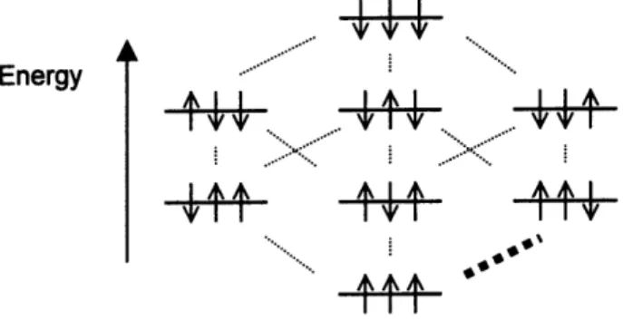
inversion. The energy level diagram for a three-spin system is shown in Figure Five. The transitions

needed by a Toffoli gate are quantum-allowed and thus able to be implemented with NMR.

Figure Five. Energy level diagram for a coupled three-spin system. The dashed lines indicate the transitions allowed by quantum mechanics. The bold line indicates a transition needed to implement a Toffoli Gate. The frequency of this transition is wc - (JAc/2) - (JAB/2.

Energy

There is a large body of theoretical work dealing with the universality of quantum gates.

Experimentally, once a method to implement the universal gate has been mastered, any computation can

be specified as a sequence of the universal gate and eventually implemented. Toffoli first proved the

universality of the three-bit gate in the classical system. Later, Deutsch proved the universality of a

quantum three-bit gate [Deutsch89]. By decomposing the quantum three-bit gate, DiVincenzo defined a

set of one- and two-bit gates as a complete quantum set [DiVincenzo94]. Barenco then decomposed the

universal quantum three-bit gate into a single type of two-bit gate [Barenco95]. He found a large class of

It is not yet known how to implement an efficient quantum computer. The following chapters

describe implementation of primitive quantum computations using NMR. It is hoped that this work will

Chapter Two. Effect of Soft Pulses On A Two-Spin System.

Hamiltonian.

The Hamiltonian is a quantum mechanical operator that describes the evolution of a system.

Evolution by the Hamiltonian is a unitary, reversible transformation. In the Schrodinger representation,

operators are time-independent and states evolve in time. This is a convenient representation to describe

NMR experiments because ideally, the Hamiltonian of the system is known and time-independent. If the

initial state of the spin system is known, the state at any future time is a solution to the Schrodinger

Equation.

In his paper describing the formalism of product operators [Sorensen83], Sorensen defines the

Hamiltonian of a transition in a two-spin system as,

Htransition - A

(1-

2L

).

In other quantum systems, the Hamiltonian associated with a transition is comprised of the term from the

excitation and the terms from the internal motion of the system. Though the transition Hamiltonian is

more convenient to use, a composite of the RF Hamiltonian (Equation Two) and the internal Hamiltonian

(Equation Four) probably represent the effective Hamiltonian of the transition more completely.

What is the effective Hamiltonian? Is there a time under which the internal Hamiltonian is

negligible? How large are the errors if instead of the effective Hamiltonian the transition Hamiltonian is

used to describe the spin system's evolution? Does the degree of spin-spin coupling influence the degree

of error?

Verification the spin system's true Hamiltonian was done. In the experiments performed, spectra

were collected from two different two-spin systems that were given RF pulses at constant frequency but

and the magnetization axis. Experimental spectra were then compared with spectra simulated using the

effective Hamitonian. The effective Hamiltonian was derived as follows:

Heffective = (HRF-rotating + Hintemal)rotating - rotation

-= * (e (I RF(IzA+I) AB*time) * RF (-'* B)RF )*JAB*time)] [-OAI - oBIB + 2nJAB B ]), T... (14)

- (coA JAB)(z +))

Equation Fourteen is simplified if the RF receiver is positioned on-resonance with the spin at wA. Alternatively, to derive the effective Hamiltonian, you can use ,

dp [p, H]+

(15)

dt 8p

Because all of the terms in the Hamiltonians commute, you can simply add the components of the RF and

internal Hamiltonians to the rotation transformation as shown in Equation Sixteen.

Heffectve = WoRF( A + I)- O IA - O)BIB +

27JABIAI

= (RF(I A +I - OAI - OBIzB + 2+JABI + ((WA + JAB)(IA + IB)) (16)

SO)RF (IA B + JAB (IA + B + 21AIB

)

Experiment Details.

Equipment. Alanine has a weak coupling between the two carbon spins highlighted in Figure Six (JAB =

35.1 Hz). 2,3-dibromothiophene (Figure Seven) has a stronger coupling between the two hydrogen spins

(JAB = 5.6 Hz). Greater coupling (a smaller JAB value) implies that a more selective RF pulse must be used. To impart the same amount of energy, a stronger coupled system needs a pulse with a lower RF

A solution of alanine in chloroform was measured with a Bruker 400 MHz spectrometer. The RF

power was set to 120 dB and the pulse length for a 900 pulse was 28.8 ms. A solution of

2,3-dibromothiophene in chloroform was measured with a Bruker 500 MHz spectrometer. The RF power was

set to 68 dB and the pulse length for a 900 pulse was 43 ms. The use of different spectrometers was dictated by convenience.

Figure Six. The chemical structure of alanine. The two marked carbons are the atoms whose spins were used in the measurement.

H

NH

Figure Seven. The chemical structure of 2,3-dibromothiophene with the two measured hydrogen atoms labeled.

H

Br

H

Br

Pulses. Standard Pound-Overhauser pulse techniques were used. The pulse sequence consisted of a

single, selective RF pulse applied either on resonance with the frequency of one of the hydrogen spins,

WA, or aligned with one of the peaks at WA ±(JAB/2). The FID was immediately collected and the Fourier transform of the FID was taken. Alanine measurements were taken at 18 equally spaced angles with the

receiver placed on the carbon's resonance frequency, WA. Nine angle measurements were taken on the

2,3-dibromothiophene sample. The RF receiver was placed at the peak, corresponding to WA + (JAB/2).

The power setting was 68 dB. With this setting, the time required to implement a 90" pulse was equal to

1/(4JAB). Experiments were done at a collection RF receiver positions and power settings. Only data from

the WA+ (JAB/2) and 68 dB experiment will be included because analysis on the other data sets is not yet

complete.

Results.

Only certain energy level transitions are allowed by the rules of quantum mechanics. In these

experiments, the area of the spectra corresponding to the allowed transitions between the 4T and Tt spin states and 11 and t4 spin states is the area of interest. These transitions are represented by the peaks at

the frequencies wA ± (JAB/2). The controlled-NOT gate is comprised of these transitions. Figures Eight

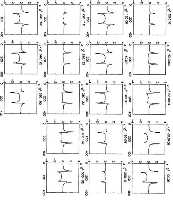
and Nine show plots of the data in the region of interest at a collection of tip angles. From left to right, the

peaks represent the populations of the I4 to T1 and 44 to "J transitions. Figures Ten and Eleven show these plots again but with spectra simulated using Equations Nine and Ten. The effective Hamiltonian

(Equation Sixteen) was used in these calculations. The spectra with the effective Hamiltonian

qualitatively agree with the experimental spectra. To discern the analytically correct Hamiltonian, a Least

Squares Fit analysis will be done on the comparison between the experimental and the simulated product

S

-~~l~~~ I. -- - --

~al-;r.,~mxr

Figure Eight. Alanine spectra. The doublet represents transitions at the frequencies CA ±+ (JABI2).

The tip angle, the angle between the spin and the magnetization axis, is shown at the top of each spectrum. Relative frequency is plotted along the x-axis. The y-axis shows the relative magnitude of the spin population that underwent the transition. In these experiments, the RF receiver was

placed at oA. M,3 0 Pi i 4 £% h0 M 0 ° i 8 8 080

r

))

it

0i

i

-

it t

11

h

t

h i

-

_ooH

I

~

A

Figure Nine. 2,3-dibromothiophene spectra. The doublet represents transitions at the frequencies

1A ± (JAB/2). The tip angle is shown at the top of each spectrum. Relative frequency is plotted

along the x-axis. The y-axis shows the relative magnitude of the spin population that underwent the

transition. In these experiments, the RF receiver was placed at CA + (JAS2).

o

0

8P

8P

8

Figure Ten. Alanine spectra with spectra simulated using Heffective,,. Tip angle is indicated at the top of the spectrum. Relative frequency is plotted along the x-axis. The y-axis shows the relative magnitude of the spin populations. The simulated spectrum is plotted with the experimental spectrum. Comparison of the spectra suggest that Heffective is the correct Hamiltonian. Notice that spectra agree at small tip angles (short RF pulses).

10 0 0 L 0 M 4L IL t'13iK) 4L M 4 LS P 4 ), H) 8. 8. C 8. " 8 8 8 0 0 0h r 0 b 00 b030 8J 80 0 0 0 0 b

0

0

[-'

Figure Eleven. 2,3-dibromothiophene spectra with spectra simulated using Heffective. Again, tip angle is indicated at the top of the spectrum, relative frequency is plotted along the x-axis and the y-axis shows the relative magnitude of the spin populations. The simulated spectrum is plotted with the experimental spectrum. Comparison of the spectra suggests that Heffectie is the correct Hamiltonian even for a more strongly coupled spin system. Differences in the spectra at large tip angles (long RF pulses) may be due to factors other than the Hamiltonian.

ci Lh 0h0 SU, , U8 8 a uo 0 1 0 0 a ci c ci 0 ci c 0~v i ci c 0 i _U, ci _{U U} 0 , ci ₀ 1 c 1 cit ₀ i 01 8 _0i i0 0& 0

To calculate the value of the product operators from the experimental spectra, the dot product of

the evolved product operator and the experimental spectrum is taken. Taking the dot product of two

vectors results in a scalar that depicts the amount of the first vector present in the second. To generate

the evolved product operator vector, the real component of the fast Fourier transform of the trace of the

product of the evolved spin density and product operator is taken. Equation Seventeen explains this

using lines from the MATLAB program used to calculate the vector of the evolved I,.

for k = 1:number_points

time = timeincrement * k

p = expm (i*H*time)* p *expm (-i*H*time) end

evolved_Ix = real (fft (trace (p lx)}) (17)

The Hamiltonian, H, is the internal Hamiltonian due to scalar coupling only (Equation Four). The time is

equal to the time between each measurement while the spectrum is being collected, or the acquisition

time divided by the number of points. The density matrix, p, is initially the density matrix of Ix but when

evaluated at each increment in time, it becomes the density of the evolved state.

The evolved product operator vector is then normalized to one. Reciprocal bases are constructed

because the measured product operators are not part of an orthogonal basis set. Once the orthogonal,

normalized product operator vectors are generated, the dot product of these unit vectors reveals the

fraction of the product operator in the experimental spectrum.

Calculations of the theoretical product operators of simulated spectra are done similarly. The only

difference is that the orthogonal, normalized product operator vectors are dotted with the vector of the

spectrum simulated using the effective (Equation Sixteen). Knowing the correct evolution of the product

operators following RF pulses will provide insight into this and other NMR pulse sequences. Plots of the

product operator versus angle for both spin systems will be made.

Calculation of the experimental product operators is still in progress. Preliminary results suggest

Data for the more weakly coupled case show the result more clearly. The spin-spin coupling effect is

more prominent in the 2,3-dibromothiophene and results in spectra with different peak magnitudes and

spin evolution. As shown in Figures Ten and Eleven, the evolution for coupled spin systems is

predictable and because quantum computations will use coupled spin systems, the results are important.

Using Results As a Logic Gate.

If the RF receiver is on-resonance with one of the transitions in the spectrum (wA ± JAB/2), application of a

180° pulse inverts the peak and results in a transitioned spin state. In the preceding experiments, the spectra corresponding to the 180" pulse represented inversion in the spin population transitioning from the

11 to the T1 state. This inversion represents the function corresponding to a controlled-NOT gate with the

output on the first spin. Inversion is clearly seen in the alanine spectrum. The first peak in the

2,3-dibromothiophene spectrum was not completely unchanged; the lineshape of the peak was changed due

to the coupling between the spins. The Hamiltonian predicts this change.

Previous experiments have implemented the controlled-NOT gate on a two- and three-spin

system using spin coherence [Cory97]. The current experiments showed the implementation of a

two-spin controlled-NOT gate using Pound-Overhauser techniques. The current experiments were important

because they confirmed suspicions that the true Hamiltonian associated with a transition is not simply the

transition Hamiltonian but more accurately, a combination of the RF and internal Hamiltonians. Because

the Hamiltonian agreed at small tip angles, it is time-independent. With the Hamiltonian of the spin

system known, and the evolution of the spin state able to be calculated with the Schrodinger Equation,

implementation of controlled-NOT gates on higher ordered spin systems is theoretically imaginable. The

Chapter Three. The Controlled-NOT Gate.

Definition.

The two-spin controlled-NOT gate with the output on the second spin represents the function: conditional on the state of the first spin, invert the state of the second spin. In the quantum regime, when coupled with an almost trivial one-bit gate, the two-spin controlled-NOT gate is universal; it can be used to build any other quantum gate [Divincenzo95], [Lloyd95], [Deutsch95]. The three-spin controlled-NOT gate obeys the rule: conditional on the state of the first and second spins, invert the state of the third spin. The n-spin controlled-NOT gate inverts the state of the nth spin conditional on the state of the first (n-1) spins.

Convenience.

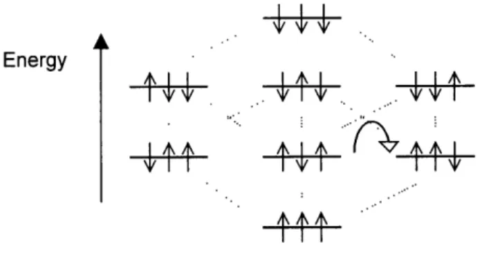
The three-spin controlled-NOT gate, the Toffoli Gate, is a universal gate in the quantum regime. Barenco showed that it can be decomposed into two two-spin gates [Barenco95-2]. The Fredkin Gate is another three-bit gate. The Fredkin Gate swaps the states of the second and third spins conditional on the state of the first spin. An example of a Fredkin transition is shown with the curved arrow in the energy level diagram for a coupled three-spin system represented in Figure Twelve.

Figure Twelve. Energy level diagram for a coupled three-spin system. Allowed transitions are

indicated with dashed lines. A transition needed to implement a Fredkin Gate is shown with a

curved arrow.

Energy

I I J-•

\Y 41 4/ V

The transition of a Fredkin Gate is not a quantum allowed transition. For this transition to be implemented

in the quantum regime, it must be decomposed into several quantum allowed transitions.

DiVincenzo and Smolin postulated that all three-bit gates can be composed of a maximum of six

two-bit gates [DiVincenzo94]. Chau and Wilczek designed the Fredkin Gate with six gates [Chau95]. Working from this result, Smolin and DiVincenzo decomposed the Fredkin Gate into five two-bit gates: a

two-bit controlled-NOT followed by a Toffoli and another two-bit controlled-NOT [Smolin96].

Reality.

A quantum two-spin controlled-NOT gate has been implemented with NMR using spin coherence

techniques. Though the universality of the quantum three-spin controlled-NOT gate was shown before

the two-spin's, the NMR implementation of the quantum three-spin controlled-NOT gate (the Toffoli Gate)

followed logically from the pulse sequence of the two-spin controlled-NOT gate. The next step was to

design spin coherence pulse sequences for n-spin controlled-NOT gates. This was done and the

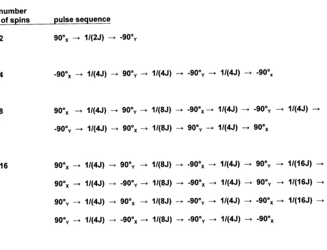
Figure Thirteen. Table of spin coherence pulse sequences for n spins. number

of spins pulse sequence 2 90*x -, 11(2J) -, -90y

4 -900x 1/(4J) 900y- 1/(4J) - 90*y - 1/(4J) -, -90x

8 90x - 1/(4J) - 900y -* 1/(8J) - -90*x-, 1/(4J) -,-90,y -- 1/(4J) -+

-90y, - 11(4J) -, 90°x -- 1/(8J) 90°y -4 11(4J) -, 90*x

16 90*x - 1/(4J) - 90*y -- 1/(8J) -90*x -, 11(4J) -, 90*y - 11(16J) -4

90x- 1/(4J) -4 -90*y -- 1/(8J) - -90ox, 11(4J) -, 90*y - 11(16J) -, 900y - 1/(4J) -4 90ox -, 1/(8J) -90°y - 1/(4J) -,-90*x -- 1/(16J) -4 90y - 1(4J) --90(4J) 1/(8J) -,90y-, 1/(4J) -9 00x

Each of the controlled-NOT pulse sequences in Figure Thirteen is valid for spin systems

containing n or less spins. The two-spin controlled-NOT gate can be implemented with any of the pulse

sequences listed. The three-spin controlled-NOT gate can be implemented with any of the sequences

except the n=2 sequence. These sequences assume a single coupling constant within a molecule.

Patterns emerge from the sequences. Any new sequence will be valid for twice the n-value of the last

sequence. Though the number of required pulses increases with an increased n sequence, the selective

halving of the delay times suggests that the increase in the total time required to implement

controlled-NOT gates does not increase exponentially. In short, while these sequences may not be the most

efficient manner in which to implement a controlled-NOT gate, the primitive controlled-NOT pulse

Using spin coherence techniques, the two- and three-spin controlled-NOT gates have been

implemented. At present, experiments to implement the four-spin controlled-NOT gate using the alanine

molecule are underway. The problems with implementing gates on higher ordered spin systems include

the need to decouple spins and refocus the previously negligible chemical shift. Experiments

Chapter Four.

Conclusions.

This is a work in progress. The comparison of the qualitative and quantitative differences

between the effective and transition Hamiltonian needs to be continued. Knowledge of product operator evolution will add to our understanding of spin systems. Plotting the different components of the product

operators versus the angle between the spin and the magnetization axis for a variety of primitive quantum

logic gates may inspire more efficient algorithms.

This discussion highlighted the controlled-NOT gate for quantum computing. Decomposing

complex gates into a series of quantum two-bit controlled-NOT gates that can be implemented with NMR,

will be an important tool in the future. The n-spin controlled-NOT gate will have utility both as its own

complete gate and as a prefix and suffix to other more complex gates. Many algorithms are dependent on

being able to execute (n -1)-spin controlled-NOT gates.

The true strength in continuing quantum computing research is that advances will be made in

secondary fields. This is witnessed by the fact that our understanding of the true Hamiltonian of a

transition was furthered by an experiment originally born out of an idea to implement a quantum gate.

Future NMR experiments on higher-ordered spin states will lead to a better understanding of spin

dynamics, more complex pulse sequences and perhaps a new way of interpreting the physics of NMR.

Ultimately, the number and complexity of the logic gates that can be performed will limit quantum

computing with NMR. The coherence time and the number of spins in a system will be important factors.

The coherence time, the time during which the system evolves in a unitary way, is dictated by the

spin-lattice relaxation,T1. As long as T1 is greater than J-1, a spin system will undergo unitary transformations.

While there are calculations that predict that the maximum number of spins able to be used in NMR

quantum computations is 73, realistically a 20-spin system should be able to perform many of the

quantum algorithms being developed. At present, the maximum number of spins that have been used in

NMR quantum computations is four. It is expected that six- and eight-spin systems will be used in the near future.

Studying the physics of the decoherence and synthesizing designer molecules may combat these

limitations. Furthermore, methods of correcting error in NMR quantum computations are underway.

While NMR has not yet been deemed the ultimate paradigm for building a quantum computer, NMR has

References.

A. Barenco. A universal two-bit gate for quantum computation. Proceedings of

the Royal Society of London A,, 1995.

A. Barenco, C Bennett, R. Cleve, D. DiVincenzo, N. Margolus, P. Shor, T. Sleator, J. Smolin and H. Weinfurter. Elementary gates for quantum computation. Physical Review A, 52:3457, 1995.

H. Chau and F. Wilczek. Realization of the Fredkin Gate using one- and two-body operators. Physical Review Letters, 50:748, 1995.

J. Cirac and P. Zeller. Quantum computations with cold trapped ions. Physical

Review Letters, 74:4091-4094, 1995.

D. Cory, M. Price, A. Fahmy and T. Havel. Ensemble quantum computing by NMR spectroscopy. Proceedings of the National Academy of Science USA, 94:199, 1997.

D. Cory, A. Fahmy and T. Havel. Nuclear Magnetic Resonance Spectroscopy: An experimentally accessible paradigm for quantum computing. Proceedings of

the Fourth Workshop on Physics and Computation. New England Complex

Systems Institute, Boston, MA, 1996.

L. Davidovich, A. Maali, M. Brune, J. Raimond and S. Haroche. Quantum

switches and nonlocal microwave fields. Physical Review Letters, 71:2360-2363, 1993.

D. Deutsch. Quantum computational networks. Proceeding of the Royal Society

of London A, 425:73, 1989.

D. Deutsch, A. Barenco and A. Ekert. Universality in quantum computation.

[DiVincenzo94] [DiVincenzo95] [Feynman82] [Gershenfeld97] [Grover96] [Lloyd93] [Lloyd95] [Shor94] [Smolin96] [Sorensen83] [Toffoli80]

D. DiVincenzo and J. Smolin. Results on two-bit gate design for quantum computers. Proceedings of the Workshop on Physics and Computation, PhysComp '94, Los Alamitos: IEEE Computer Science Press, p. 14, 1994.

D. DiVincenzo. Two-bit gates are universal for quantum computation. Physical

Review Letters, 50:1015, 1995.

R. Feynman. Simulating physics with computers. International Journal of

Theoretical Physics, 21:467-488.

N. Gershenfeld and I. Chuang. Bulk spin resonance quantum computation.

Science, 275:350-356, 1997

L. Grover. A fast quantum mechanical algorithm for database search. Journal

of Ref.: Proceedings, 2 8th Annual ACM Symposium on the Theory of Computing

(STOC), pp.212-219, May 1996.

S. Lloyd. A potentially realizable quantum computer. Science, 261:1569, 1993.

S. Lloyd. Almost any quantum logic gate is universal. Physical Review Letters, 75:346-349, 1995.

P. Shor. Algorithms for quantum computation: discrete log and factoring. 35th

Annual Symposium on Foundations of Computer Science, Ed. Shafi Goldwasser,

IEEE Press, pp. 124-134, 1994.

J. Smolin and D. DiVincenzo. Five two-bit quantum gates are sufficient to implement the quantum Fredkin Gate. Physical Review A, 53:2855, 1996.

O. Sorensen, G Eich, M. Levitt, G. Bodenhausen and R. Ernst. Product operator formalism for the description of NMR pulse experiments. Progress in NMR

Spectroscopy, 16:163-192, 1983.

T. Toffoli. Reversible computing. Automata, Languages and Programming, Eds. J de Bakker and J. van Leeuwen, Springer-Verlag, pp.632-644, 1980.