HAL Id: hal-01094700
https://hal.inria.fr/hal-01094700
Submitted on 12 Dec 2014
HAL is a multi-disciplinary open access
archive for the deposit and dissemination of
sci-entific research documents, whether they are
pub-lished or not. The documents may come from
teaching and research institutions in France or
abroad, or from public or private research centers.
L’archive ouverte pluridisciplinaire HAL, est
destinée au dépôt et à la diffusion de documents
scientifiques de niveau recherche, publiés ou non,
émanant des établissements d’enseignement et de
recherche français ou étrangers, des laboratoires
publics ou privés.
Modelling thermal adaptation in microalgae : an
adaptive dynamics point of view
Ghjuvan Micaelu Grimaud, Francis Mairet, Olivier Bernard
To cite this version:
Ghjuvan Micaelu Grimaud, Francis Mairet, Olivier Bernard. Modelling thermal adaptation in
mi-croalgae : an adaptive dynamics point of view. 19th IFAC World Congress, Aug 2014, Cape Town,
South Africa. pp.4376-4381, �10.3182/20140824-6-ZA-1003.00982�. �hal-01094700�
Modelling thermal adaptation in microalgae
: an adaptive dynamics point of view
Ghjuvan Micaelu Grimaud ∗,⋆ Francis Mairet ∗,⋆ Olivier Bernard∗
∗BIOCORE-INRIA, BP93, 06902 Sophia-Antipolis Cedex, France
Abstract: Controlling microalgae outdoor cultures is a growing challenge as these organisms
could be used at the industrial scale to produce biofuels. In this context, understanding how temperature affects microalgae is a major field. Because of their high division rate, microalgae rapidly adapt to their environment through a process of selection - mutation so that it is not possible to neglect the evolution part. We present here a simple Monod-like model to account for temperature effect on microalgae. We then use it in an evolutionary perspective thanks to the Adaptive Dynamics theory to understand how temperature drives evolution. We analyze the model for a constant temperature, showing that the optimal temperature trait tends to equal the environment temperature. We then study the case where the temperature is periodically fluctuating, and we find a stable equilibrium. Finally, we simulate the model to show that evolutionary branching in two distinct morphs can occur under this condition, which could be a first step to find a criterion for strain selection.
Keywords: temperature, evolution, adaptive dynamics theory, microalgae
1. INTRODUCTION
Autotrophic micro-organisms called ‘microalgae’ brought together a variety of unicellular photosynthetic eukaryotes. Some of them are able to accumulate an important amount of neutral lipids (Mata et al., 2010), which can be turned into biofuel, others can store important quantities of carbohydrates, used for methane production. Thus, they are a promising biotechnology resource for the future (Wijffels et al., 2013). Their growth is mostly influenced by light, but temperature is the second determining factor because microalgae are ectotherms (i.e they can’t regulate their internal temperature). The temperature effect on growth is often neglected in the modelling of microalgae. In regard to the increasing interest for outdoor production of microalgae, temperature effect on growth has to be investigated (Ras et al., 2013).
Because of their high division rate, microalgae are able to rapidly adapt to their environment through a process of selection - mutation. In outdoor cultures, the daily range of temperature fluctuation can be more than 20◦C (Bechet et al., 2010). It is thus important to understand how temperature drives evolution. To date, there is only one model which predicts microalgae adaptation to tempera-ture (Thomas et al., 2012), by simulations based on the Adaptive Dynamics theory. However, this model implies several assumptions that have been put in doubt (Boyd et al., 2013).
We propose here a simple Monod-like model that repre-sents the effect of a constant temperature on growth. We employ it to model microalgae adaptation to temperature. In line with Thomas et al. (2012), we use the Adaptive ⋆ Corresponding authors {ghjuvan.grimaud, fran-cis.mairet}@inria.fr
Dynamics theory. We keep the model as simple as possible to study it analytically. In a second part, we use the model under periodic temperature to account for more realistic conditions. Finally, we simulate strain separation through evolutionary branching under fluctuating temperature.
2. MODELLING TEMPERATURE EFFECT ON MICROALGAE GROWTH
The influence of temperature on all ectotherms growth is a well-known asymetric curve, called thermal reaction norm (Fig. 1 A). In microalgae, two models have been used to describe temperature effect on growth (Norberg, 2004; Bernard and R´emond, 2012). We use the model from Bernard and R´emond (2012) based on the Cardinal Temperature Model with Inflection (CTMI) of Rosso et al. (1993) because its parameters can be directly estimated on the available data:
µ(T ) = 0 for T < Tmin µopt λ(T )
β(T ) for Tmin< T < Tmax
0 for T > Tmax (1) with λ(T ) = (T− Tmax)(T − Tmin)2 β(T ) = (Topt− Tmin) [
(Topt− Tmin)(T− Topt)
−(Topt− Tmax)(Topt+ Tmin− 2T )
] (2)
Topt>
Tmin+ Tmax
2 (3)
T corresponds to the temperature of the environment, µ(T ) is the growth rate of a given species, Tminand Tmax
are the minimum and maximum temperatures that sustain growth, Topt is the optimal temperature for growth and
µoptis the theoretical maximum growth rate. Contrary to
Norberg (2004) used in Thomas et al. (2012), this model does not imply any assumption concerning the structural link between the cardinal temperatures and the maximal growth rate (e.g. if Topt is hotter, µoptwill be higher).
In the following, we use a Monod-type model including the temperature effect on microalgae growth in a chemostat:
M :
{ ˙
S = D(Sin− S) − µ(T )ρ(S)X
˙
X = µ(T )ρ(S)X− DX (4)
where S is the nutrient concentration in the chemostat, X is the algal biomass concentration, D is the dilution rate and with:
ρ(S) = S
K + S (5)
K is a half-saturation coefficient.
It is possible to calculate the non zero equilibrium (S∗, X∗) of system (M ):
S∗ = KD
µ(T )− D X∗ = (Sin− S∗)
(6)
with the hypothesis µ(T )ρ(Sin)− D > 0.
In the following, we use a Lyapunov function taken from Harisson (1979) to prove that (6) is globally asymptotically stable.
Lemma 1. The Lyapunov candidate function is given:
V (S, X) = ∫ S S∗ µ(T )ρ(w)− µ(T )ρ(S∗) µ(T )ρ(w) dw + ∫ X X∗ w− X∗ w dw (7)
with V : B→ R2where B is an open containing (S∗, X∗).
V (S, X) is zero at (S∗, X∗), positive at all other points (S, X), defined and monotone increasing when |X − X∗| or |S − S∗| increases. The time derivative of V is:
˙ V (S, X) = 1 µ(T )ρ(S)(D− µ(T )ρ(S)) [ µ(T )ρ(S) (Sin− S∗)− D(Sin− S) ] (8)
Proof: It is obvious that V (S∗, X∗) = 0. Moreover, since the integrands are of the same sign as X− X∗ and S− S∗, the integrals are positive and increasing as|X − X∗| and
|S − S∗| increase.
Proposition 2. If D < µ(T )ρ(Sin), System (M ) admits
one non zero equilibrium which is globally asymptotically stable.
Proof: It is sufficient to prove that (8)< 0∀(S, X) ∈ B,
(S, X)̸= (S∗, X∗).
If S > S∗ (resp. S < S∗), then D− µ(T )ρ(S) < 0 (resp.
> 0) because µ(T )ρ(S∗) = D, and[µ(T )ρ(S)(Sin− S∗)−
D(Sin− S)
]
> 0 (resp. < 0) because Sin− S < Sin− S∗
(resp. Sin− S > Sin− S∗). Thus, (8)< 0 is verified, and
(S∗, X∗) is globally asympotitcally stable.
3. EVOLUTIONARY MODEL
3.1 General case
We now study the system (M ) in the context of adaptive dynamics, introducing a mutant Xmut with an adaptive
trait amut (i.e. a quantifiable trait that is likely to evolve)
different from the resident trait a, with µmut(amut, T )
and µ(a, T ) (Dieckmann and Law, 1996). For further introduction to adaptive dynamics, see Dieckmann (2004). To define the canonical equation of adaptive dynamics, i.e. the equation of the evolution of trait a (Dieckmann and Law, 1996), we need to find the mutant growth rate (per
capita) in the resident population at equilibrium, called
invasion fitness f (amut, a).
Proposition 3. The invasion fitness for System (4) is given
by: f (amut, a) = D ( λmut λ β βmut − 1 ) (9)
Proof: This results from the steady-state condition of the
resident system, and from the hypothesis that the mutant is initially rare. We can thus replace S by its equilibrium value S∗:
f (amut, a) = µmut(amut, T )ρ(S∗)− D (10)
3.2 Modelling the evolution of the optimal temperature trait
We choose to study the adaptive trait a = Topt, assuming
that temperature will mainly affect the optimal conditions for growth. Because of the constraint (3) on Topt, we choose
to study the case:
T > Tmin+ Tmax
2 (11)
We calculate the selection gradient, which gives the direc-tion of the selecdirec-tion, using (9):
∂f (amut, a) ∂amut amut=a =−β ′(a) β(a)D (12) with β′(a) =−6a2+ (6T + 2T max+ 4Tmin)a +(−2Tmax− 4Tmin)T (13) We can deduce the canonical equation of the adaptive trait, that describes the evolution of Topt at the
da
dθ =−Mpσ
2X∗D β′(a)
β(a) (14)
where Mp is the probability to be a mutant at each
apparition, and σ is the mutation step.
We then search for the evolutionary singular strategy. We find that da/dθ = 0 for a∗ = T , which means that the optimal temperature trait tends to equal the environment temperature (Fig. 1 B). Note that the same results can be obtained with the Droop model (not presented here for sake of brevity).
We investigate the stability of the singular strategy exam-ining the sign of the fitness invasion second order deriva-tive.
Proposition 4. a∗ is Convergent Stable Strategy (CSS), which means that the singular strategy is attractive, and Evolutionary Stable Strategy (ESS), which means that the resident a∗ can’t be invade by another mutant.
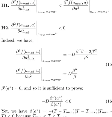
Proof: The following conditions are respected: H1. ∂ 2f (a mut, a) ∂a2 mut amut=a=a∗ < ∂ 2f (a mut, a) ∂a2 amut=a=a∗ H2. ∂ 2f (a mut, a) ∂a2 mut amut=a=a∗ < 0 Indeed, we have: ∂2f (a mut, a) ∂a2 mut amut=a=a∗ =−Dβ ′′β− 2β′2 β2 ∂2f (amut, a) ∂a2 amut=a=a∗ = Dβ ′′ β (15)
β′(a∗) = 0, and so it is sufficient to prove:
−Dβ′′(a∗)
β(a∗) < 0 (16) Yet, we have β(a∗) = −(T − Tmin)(T − Tmax)(Tmin −
T ) < 0 because Tmin< T < Tmax.
Also, β′′(a∗) = 2Tmax + 4Tmin − 6T . β′′(a∗) < 0 is
equivalent to T > (2Tmin+ Tmax)/3 which is true because
of (11). Thus, (16) is true. H1 and H2 are verified.
3.3 Structural link between adaptive traits
In a real case of evolution, it is possible that several adaptive traits evolve concurrently, e.g. Tmaxand Topt. In
bacteria, Rosso et al. (1993) point out that there exists a structural link between Tmax and Topt. That is, Tmax can
be written as a linear function of Topt. We compiled data
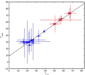
from Miller and Castenholz (2000) for cyanobacteria and from Bernard and R´emond (2012) for microalgae to verify whether this relation is true for these organisms (Fig. 2). The data reveal a good correlation:
Tmax= mTopt+ p (17)
with m = 0.93 and p = 9.83, r = 0.941 (Fig. 2). This property must depend on the genetic interactions between traits, but the exact reason for such a link is still to understand.
In expression (9), we replace Tmaxby (17). By taking the
adaptive trait a = Topt, the selection gradient becomes:
∂f (amut, a) ∂amut amut=a = Dλ ′(a)β(a)− β′(a)λ(a) λ(a)β(a) (18) with λ′(a) =−m(T − Tmin)2 (19)
We search for the evolutionary singular strategy by setting Eq.(18) equal to zero. As for (14), we find that a∗ = T , and thus Tmax∗ = mT + p (Fig. 1 C). This is an impor-tant result in the context of co-evolving species, because whether Tmaxevolve or not, the thermal reaction norm will
differently affect the species fitness in its environment, and so its competition with other species or stains.
4. FLUCTUATING TEMPERATURE
4.1 Ecological timescale
We now study the system (M ) in the context of fluctuating temperature:
{
T = Tinf if t mod τ∈ [ϵ; τ1− ϵ[
T = Tsupp if t mod τ ∈ [τ1+ ϵ; τ− ϵ] (20)
with Tinf < Tsupp. By applying the conservation principle,
we have the equality X + S = Sin at equilibrium, that is
to say S = Sin− X. Thus, the system (M) can be reduced
to a one dimension differential equation: ˙ X = [µ(T (t))ρ(Sin− X) − D]X (21) 5 10 15 20 25 30 35 0 0.2 0.4 0.6 0.8 1 Temperature (°C)
Normalized growth rate (t
−1 ) T min A C B T max T opt a*
Fig. 1. Thermal reaction norm for Nannochloropsis oceanica (A). (B) and (C) are the evolutionary cases for T = 30◦C with a∗= T , and with Tmax= ma∗+ p for (C). The black circles
0 10 20 30 40 50 60 70 80 −10 0 10 20 30 40 50 60 70 80 90 T opt Tmax
Fig. 2. Linear relationship between Tmax and Topt. Data from
Bernard and R´emond (2012) are represented in blue, data from Miller and Castenholz (2000) are in red. From Miller and Castenholz (2000), we took data for the Synechococcus strains C9, SH94, OH2,20,30,29,28,4. Vertical and horizontal bars errors are represented, computed with the same method as Bernard and R´emond (2012).
where T (t) is given by Eq. (20). We define g(t, X) def=
µ(T (t))ρ(Sin− X) − D.
We follow the same reasoning as Butler et al. (1985) and Butler and Freedman (1981) who study a similar Monod-type model, but with a time varying dilution rate
D(t) instead, and a predator-prey system with periodic
coefficients, respectively.
Theorem 1: For D < min(µ(T)ρ(Sin), equation (21) has
a unique nontrivial positive periodic solution ψ(t) which is globally orbitally asymptotically stable. Moreover, we have mins∈[0,τ]A(s)≤ ψ(t) ≤ maxs∈[0,τ]A(s) with
A(t) := [D(Sin+ K)− µ(T (t))Sin]/(D− µ(T (t))
(which corresponds to the steady state biomass concentra-tion for constant T ).
Proof: ∂g/∂X exists and is continuous for (t, X)∈ R1×
R1+with R1+={X ∈ R1: X≥ 0}.
Moreover, ∃A(t) > 0 ∋ [X − A(t)]g(t, X) < 0 ∀X > 0, X ̸= A(t). Indeed, given D < min(µ(T)ρ(Sin), we have:
[X− A(t)] g(t, X) < 0
∀X > 0, X ̸= A(t) (22)
Thus, Massera’s theorem (Massera, 1950) easily implies the existence of a periodic solution ψ(t) of (21) satisfying mins∈[0,τ]A(s)≤ ψ(t) ≤ maxs∈[0,τ]A(s).
ψ(t) is the unique solution of (21), given that X∂g(t, X)/∂X <
0 for all (t, X)∈ R1× R1+. Indeed, we have:
X∂g(t, X)
∂X = µ(T )X
−K
(Sin− X + K)2
(23) Because X > 0, K > 0, X∂g(t, X)/∂X < 0 is always veri-fied. Following the same reasoning as Butler and Freedman (1981), X∂g(t, X)/∂X < 0 implies that g(t, X) is strictly
decreasing as a function of X, for X > 0, for all t. So, if two solutions ψ(t) and ψ2(t) exist, with ψ(t) < ψ2(t), it implies
that ψ′(t)/ψ(t) = g(t, ψ(t)) > g(t, ψ2(t)) = ψ2′(t)/ψ2(t)
for all t. Integrating this inequality over [0, τ ] leads to a contradiction which prove the uniqueness of ψ(t).
Using theorem 1, we have the following inequality with the periodic temperature (20): D(Sin+ K)− µ(Tinf)Sin D− µ(Tinf) ≤ X(t) ≤D(Sin+ K)− µ(Tsupp)Sin D− µ(Tsupp) (24)
which means that
DK
µ(Tinf)− D ≤ S(t) ≤
DK µ(Tsupp)− D
(25) If the time spent at each temperature is sufficiently long, then, when T = Tinf (resp. T = Tsupp), the substrate
concentration converges towards its equilibrium Sinf∗ =
DK/(µ(Tinf)−D) (resp. Ssupp∗ = DK/(µ(Tsupp)−D)). We
assume that the state transition between S∗inf and Ssupp∗ is negligible. From a biological point of view, this assumption implies that the growth rates at both temperatures are quite similar.
4.2 Evolutionary timescale
As explained previously, we assume that the resident popu-lation reaches rapidly its equilibrium for each temperature applied. In the case with the adaptive trait a = Topt and
considering a constant Tmax, we obtain:
f (amut, a) = D ( β(Tinf) βmut(Tinf) − 1 ) if T = Tinf f (amut, a) = D ( β(Tsupp) βmut(Tsupp)− 1 ) if T = Tsupp (26)
It is possible to use the average mutant growth rate in the resident population at steady-state (Ripa and Dieckmann, 2013): ¯ f (amut, a) = 1 τ ∫ τ 0 f (amut, a; t) dt
which is equivalent to:
¯
f (amut, a) = D
[
β(a, Tinf)
β(amut, Tinf)
τ1
τ
+ β(a, Tsupp)
β(amut, Tsupp)
τ− τ1
τ − 1
] (27)
We thus deduce the selection gradient:
∂ ¯f (amut, a) ∂amut amut=a = D [ −τ1 τ β′(Tinf) β(Tinf)− τ− τ1 τ β′(Tsupp) β(Tsupp) ] (28)
Table 1. Model parameters for evolutionary branching.
Parameters Unit
Tmin, minimal temperature for growth 4◦C
Tmax, maximall temperature for growth 40◦C
Tinf, inferior temperature applyed 20◦C
Tsupp, superior temperature applyed 36◦C
τ1, time during which Tinf is applyed 12 h τ , period of temperature fluctuation 24 h
and so the canonical equation of the adaptive trait with fluctuating temperature is:
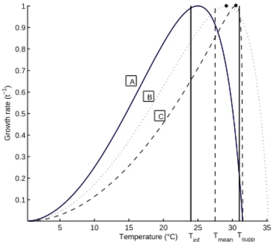
da dθ = Mpσ ¯X ∗∂ ¯f (amut, a) ∂amut amut=a (29) Equation (29) is not analytically tractable. We perform simulations of (29) to search for the evolutionary singular strategy. Result (Fig. 3 C) shows that, at steady, Topt
does not converge to the average temperature Tmean. This
result is still available if we replace Tmax by a linear
function of Topt (Fig. 3 B), even if a∗ is different. The
asymmetric property of the thermal reaction norm is probably the reason for such outcome.
5 10 15 20 25 30 35 0.1 0.2 0.3 0.4 0.5 0.6 0.7 0.8 0.9 1 Temperature (°C) Growth rate (t −1 ) B C A T supp T inf Tmean
Fig. 3. Evolution of the thermal reaction norm for Tinf = 24◦C, Tsupp = 31◦C. (A) is the initial reaction norm, (B) is the evolutionary reaction norm for a = Toptand Tmax= mTopt+ p
at steady-state, and (C) is the evolutionary reaction norm for
a = Topt and Tmax = 31.5◦C at steady state. The singular
strategies are represented by black points.
4.3 Evolutionary Branching conditions
Under particular conditions, Adaptive Dynamics predict that evolution can converge to a specific singular strategy called ‘branching point’ where selection becomes disrup-tive, so that two strains move apart (Metz et al., 1992). The mutant can invade the resident and reciprocally, and both stably coexist.
We investigate the evolutionary dynamics of (3) by using a pairwise invasibility plot (PIP) (Fig. 4)(Geritz et al., 1998). This allow us to determine the stability of the singular strategy, studying graphically the sign of the mu-tant invasion fitness. For temperatures comprised between
Tinf = 20◦C and Tsupp = 36◦C, and with Tmin = 4◦C,
Tmax = 40◦C, we find that there exist a branching point
(Fig. 4 A). Indeed, at this point, mutant and resident
a amut 20 25 30 35 40 20 25 30 35 40 a amut 20 25 30 35 40 20 25 30 35 40 a amut 20 25 30 35 40 20 25 30 35 40 a amut 20 25 30 35 40 20 25 30 35 40 + + + + + + + + B D C A Tinf= 18, Tsupp=38 T
inf= 17, Tsupp=39 Tinf= 16, Tsupp=40
T
inf= 20, Tsupp=36
Fig. 4.Pairwise Invasibility Plots across a range of values of Tinf
and Tsupp (expressed in◦C). The other parameters are listed
in Table 1. Grey and white represent positive and negative invasion fitness, respectively. Evolutionary singular strategy are represented by a black circle.
can mutually invade in such a way that two strains sep-arate. For a range of values around the previous ones, we observe that the singular strategy bifurcates in three singular strategies (Fig. 4 B, C, D). In Fig. 4 D, there is still a branching point, which seems to allow a strong separation between strains because of the large area of positive invasion fitness.
To confirm the results found previously, we perform a simulation of an evolutionary branching. In line with Mirrahimi et al. (2011), we consider a model where the adaptive trait a becomes a continuous trait:
Fig. 5.Evolutionary branching of trait a for the parameters of Table 1. The trait a is expressed in◦C, t is arbitrarily expressed in hours. The colored lines correspond to a population size for each trait value.
∂tX(a, t) = X(a, t)[µ(a, T )S(t)− D] + ϵ∆X(a, t)
S(t) = DSin
D +∫µ(a, T )X(a, t) da
(30)
where X(a, t) is the species density with trait a = Topt,
S(t) is the quasi-static approximation of resource
in Table 1. Fig. 5 shows that an evolutionary branching really occurs. Two general morphs with two distinct Topt
appear and stabilize.
5. CONCLUSION
We have proposed a simple model of temperature effect on microalgae growth based on the model developped by Bernard and R´emond (2012). We used it in an evolutionary perspective thanks to the adaptive dynamics. We found that, under constant temperature, the optimal tempera-ture tends to equal the environment temperatempera-ture.
In a second part, we showed that there exists a structural link between Tmaxand Topt. In the evolutionary sense, the
optimal temperature also tends to the environment tem-perature, but the thermal reaction norm is different. Thus, the outcome of evolution if several microalgae species coexist is mostly influenced by this structural link, which may differ between species depending upon the genetics and physiological constraints.
Finally, we studied our model under a simple fluctuating temperature signal. We showed that a stable periodic solution exists. At evolutionary time scale, the fluctuating temperature allows strains to separate, and evolutionary branching occurs. We simulated the strain separation and found results consistent with our theoretical approach. This may be a first step to understand how species coexist under fluctuating temperature. It could serve to find a criterion for selecting species with the highest growth rate under particular temperature conditions, which is of key interest for microalgae outdoor production.
ACKNOWLEDGEMENTS
This work was supported by the ANR Facteur 4 project. REFERENCES
Bechet, Q., Shilton, A., Fringer, B., Munoz, R., and Guieysse, B. (2010). Mechanistic modeling of broth tem-perature in outdoor photobioreactors. Environmental
science and technology, 44, 2197–2203.
Bernard, O. and R´emond, B. (2012). Validation of a simple model accounting for light and temperature effect on microalgal growth. Bioresource Technology, 123, 520– 527.
Boyd, P.W., Rynearson, T.A., Armstrong, E.A., Fu, F., Hayashi, K., Hu, Z., Hutchins, D.A., Kudela, R.M., Litchman, E., Mulholland, M.R., Passow, U., Strzepek, R.F., Whittaker, K.A., Yu, E., and Thomas, M.K. (2013). Marine phytoplankton temperature versus growth responses from polar to tropical waters outcome of a scientific community-wide study. PLoS ONE, 8, e63091. doi:10.1371/journal.pone.0063091.
Butler, G. and Freedman, H. (1981). Predator-prey system with periodic coefficients. Mathematical biosciences, 55, 27–38.
Butler, G., Hsu, S., and Waltman, P. (1985). A mathe-matical model of the chemostat with periodic washout rate. SIAM J. Appl. Math., 45, 435–449.
Dieckmann, U. (2004). A beginners guide to adaptive dynamics. in Mathematical modelling of population
dy-namics, R. Rudnicki (ed.). Banach Center Publications, no. 63. Polish Academy of Sciences, Warsaw.
Dieckmann, U. and Law, R. (1996). The dynamical theory of coevolution: A derivation from stochastic ecological processes. Journal of Mathematical Biology, 34, 579– 612.
Geritz, S., Kisdi, E., Mesz´ena, G., and Metz, J. (1998). Evolutionarily singular strategies and the adaptive growth and branching of the evolutionary tree.
Evo-lutionary Ecology, 12, 35–57.
Harisson, G. (1979). Global stability of predator-prey interactions. J. Math. Biology, 8, 159–171.
Massera, J. (1950). The existence of periodic solutions of systems of differential equations. Duke Math. J., 17, 457–475.
Mata, T., Martins, A.A., and S., C.N. (2010). Microal-gae for biodiesel production and other applications: a review. Renew Sustainable Energy Rev, 14, 217–232. Metz, J.A.J., Nisbet, R., and Geritz, S. (1992). How should
we define fitness for general ecological scenarios ? Trends
in Ecology and Evolution, 7, 4222–4229.
Miller, S. and Castenholz, R. (2000). Evolution of ther-motolerance in hot spring cyanobacteria of the genus
Synechococcus. Appl. and Env. Micr., 66, 4222–4229.
Mirrahimi, S., Perthame, B., and Wakano, J. (2011). Evolution of species trait through resource competition.
J. Math. Biol., 64, 1189–1223.
doi:10.1007/s00285-011-0447-z.
Norberg, J. (2004). Biodiversity and ecosystem function-ing: A complex adaptive systems approach. Limnol Oceanogr, 49, 1269–1277.
Ras, M., Steyer, J., and Bernard, O. (2013). Tempera-ture effect on microalgae: a crucial factor for outdoor production. Reviews in Environmental Science and Bio/Technology, 12, 153–164.
Ripa, J. and Dieckmann, U. (2013). Mutant invasions and adaptive dynamics in variable environments. Evolution, 67, 1279–1290. doi:10.1111/evo.12046.
Rosso, L., Lobry, J., and Flandrois, J. (1993). An un-expected correlation between cardinal temperatures of microbial growth highlighted by a new model. J Theor
Biol, 162, 447–463.
Sandnes, J., Kllqvist, T., Wenner, D., and Gislerod, H. (2005). Combined influence of light and temperature on growth rates of Nannochloropsis oceanica: linking cellu-lar responses to cellu-large-scale biomass production. Journal
of Applied Phycology, 17, 515–525.
doi:10.1007/s10811-005-9002-x.
Thomas, M., Kremer, C., Klausmeier, C., and Litchman, E. (2012). A global pattern of thermal adaptation in marine phytoplankton. Science, 338, 1085–1088. Wijffels, R., Kruse, O., and Hellingwerf, K. (2013).
Poten-tial of industrial biotechnology with cyanobacteria and eukaryotic microalgae. Current Opinion in