Development of a sustainable transmission structure replacement and maintenance strategy

-1

Development of a Sustainable Transmission Structure

Replacement and Maintenance Strategy

By

Max Tuttman

Sc.B. Mechanical Engineering, Brown University, 2009

SUBMITTED TO THE MIT SLOAN SCHOOL OF MANAGEMENT AND THE DEPARTMENT OF

MECHANICAL ENGINEERING IN PARTIAL FULFILLMENT OF THE REQUIREMENTS FOR

THE DEGREES OF

MASTER OF BUSINESS ADMINISTRATION

AND

MASTER OF SCIENCE IN MECHANICAL ENGINEERING

IN CONJUCTION WITH THE LEADERS FOR GLOBAL OPERATIONS PROGRAM AT THE

MASSACHUSETTS INSTITUTE OF TECHNOLOGY

JUNE 2018

@2018 Max Tuttman. All rights reserved.

The author hereby grants to MIT permission to reproduce and to distribute publicly paper and electronic copies of this thesis document in whole or in part in any medium now

known or hereafter created.

Signature of Author:

Signature redacted

Department of Mechanical Engineering, MIT Sloan School of Management

May 11, 2018

Certified by:

I

CUULCU

Georgia Perakis, Thesis Supervisor

Certified by:

Signature redacted

William F. Pounds Professor of Management

Accepted by:

Accepted by:

.~-,-' I~

~ignature

Konstantin Turitsyn, Thesis Supervisor

red

acted

~ssor of Mechanical Engineering

Rohan Abeyaratne

/

,Chair. Mechanical Enaineerina Graduate Program Committee

Signature

redacted

MASSACHSM ILNS TUTE

OF TECHNOLOGY

JUN

7

2018

LIBRARIES

Maura Herson

Director, MBA Program

MIT Sloan School of Management

0

Development of a Sustainable Transmission Structure

Replacement and Maintenance Strategy

By

Max Tuttman

Submitted to MIT Sloan School of Management on May 11, 2018 in Partial Fulfillment of the

requirements for the Degrees of Master of Business Administration and Master of Science in Mechanical Engineering.

ABSTRACT

This thesis proposes methods to both estimate optimal aggregate investment levels for a system of transmission towers by means of an integrated corrosion and failure simulation as well as a method to identify specific assets in need of investment through a statistical model of structural health. Limited tower replacements over the past decade have resulted in an overall aging of PG&E's transmission system, leading to managerial concerns about potential increased maintenance and replacement costs going forward. The utility is seeking to be able to forecast its future needs despite a minimal history of asset failure.

This work establishes long-term investment scenarios by simulating asset aging due to atmospheric corrosion and integrating those simulations with maintenance, replacement, and failure cost

estimates. In addition, the aggregate investment forecasts are supplemented with an asset health ranking methodology that enables more targeted resource deployment.

Implementation of the simulation based forecasting provides long-term spend estimates - on the order of many decades - and enables the production of sensitivity analyses based on underlying parameters grounded in physical system properties. This advances current industry spend forecasting which relies on qualitative risk assessments and past cost trends. Asset health indices generated from structural properties and environmental data are also shown to correctly rank a structure with a historic reported structural issue as at higher risk than a structure without a reported issue at a rate of 70%.

Thesis Supervisor: Georgia Perakis

Title: William F. Pounds Professor of Management

Thesis Supervisor: Konstantin Turitsyn Title Professor of Mechanical Engineering

Acknowledgements

I would like to thank all of those who supported this thesis and helped me find my way at PG&E. This includes the project champion Eric Back, whose clear vision for this project and availability throughout made my time at the company an enjoyable and frictionless experience. I would also like to thank Greg Gabbard and the rest of the transmission operations team for bringing me into their work. This project could also not have been done without the input of Dave Gabbard and his asset strategy team, including Boris Andino and Feven Mihretu.

I would further like to thank my MIT advisors Professor Georgia Perakis and Professor Kostantin Turitsyn for their support and input throughout the past year.

I am immeasurably grateful to the exceptional peers that I have had throughout my academic life including those at LGO. I am humbled and inspired by both your excellence and your character. Most of all thank you to my parents and my wife, Zahra, for your patience and love.

Contents

1

1.1 Com pany Overview ... 14

1.2 Industry Background and M otivation... 14

1.2.1 State of Electric Grid Infrastructure... 14

1.2.2 Regulatory Environm ent...14

1.3 Problem Statem ent and Objectives...15

1.4 Thesis Contribution...15

1.5 Thesis Outline...16

2 Literature Review ... 17

2.1 C orrosion in the U tility Industry...17

2.2 M achine Learning for Asset Inspections... 17

2.3 A sset M anagem ent of Transm ission Tow ers... 17

3 Steel Structure Budget Forecasting ... 21

3.1 Forecasting Approach and M odel Structure ... 21

3.2 C orrosion M odeling...22

3.2.1 General Corrosion Background ... 22

3.2.2 Corrosion Calculation M ethodologies... 23

3.2.3 ISO M odel Im plem entation ... 25

3.2.4 Structure Properties...27

3.2.5 Corrosion M odel Output...27

3.3 Single Structure Sim ulation ... 28

3.3.1 Failure Likelihood Estim ation... 28

3.3.2 M odeling Life Cycle Events...29

3.3.3 Cost Estim ates...30 7

3.3.4 T ow er Life Cycle Sim ulation ... 31

3.4 M aintenance and Replacem ent O ptim ization ... 33

3.5 System Sim ulation ... 36

3.5.1 System Sim ulation Inputs ... 36

3.5.2 Sim ulation Execution ... 39

3.5.3 Spend Forecast ... 39

3.6 Conclusions ... 44

4 Investm ent Breakeven A nalysis ... 46

4.1 Form ulation ... 46

4.2 Calculating Failure Probability ... 48

4.3 Maintenance Breakeven Analysis of Steel Transmission Structures ... 49

4.4 Conclusions ... 50

5 A sset H ealth M odeling ... 51

5.1 M odel M otivation ... 51

5.2 D ata O verview ... 51

5.2.1 Asset Data - PG&E GIS System and Asset Inventory ... 51

5.2.2 Environm ental D ata ... 52

5.2.3 Inspection R ecords ... 53

5.3 M odel Construction ... 56

5.3.1 M odeling M ethodology ... 56

5.3.2 T raining D ata ... 56

5.3.3 V ariable Selection ... 57

5.3.4 M odel Coeffi cients ... 57

5.4 M odel Perform ance ... 59

5.5 V isualizing R esults ... 61

5.6 Conclusions ... 63

6.1 Inspection and D ata Collection ... 64

6.2 T argeted Inspection and M aintenance Scheduling ... 64

6.3 Cost of Failure Estim ation ... 64

6.4 Failure M ode A nalysis ... 65

6.5 Foundation H ealth A nalysis...65

List of Figures

F igu re 1 : B PA R isk M atrix ... 1 8

Figure 2: Transpower Condition Assessment Degradation Rate Curves ... 19

Figure 3: Transpower Degradation Modeling Example ... 20

F ig u re 4 : F o recast F lo w ... 2 2 Figure 5: Landolfo's Comparison of Corrosion Model Predictions for Five and Twenty Years...24

Figure 6: Section Loss over Time ... 28

Figure 7: Tower Failure Distribution ... 29

Figure 8: Tower Maintenance Cost Curve ... 31

Figure 9: Tower Aging Simulation Flow Diagram ... 32

Figure 10: Example Tower Simulation ... 33

Figure 11: Maintenance Plan Discounted Costs... 34

Figure 12: Optimal Maintenance Schedule Parameters ... 35

Figure 13: Tower in Corrosion Zone 6 after 5 years... 36

Figure 14: PG&E Corrosion Map - San Francisco County... 37

Figure 15: Assets by Corrosion Zone...38

Figure 16: Structure Installation Year ... 39

Figure 17: Asset Cost Events...40

Figure 18: Cost Projection by Event Type ... 41

Figure 19: Cost Projection by Corrosion Zone... 42

Figure 20: Asset Failures over Time by Failure Cost Factor... 43

Figure 21: Repairs over Time by Failure Cost Factor ... 43

Figure 22: Optimized System NPV Costs as a Function of Failure Multiple ... 44

Figure 23: Tower Life Estimates ... 49

Figure 24: Breakeven Restoration Cost by Age... 50

Figure 25: Notification Cleansing...55

Figure 26: Forward Variable Selection Schematic... 57

Figure 27: Model Summary...58

Figure 28: Impact of Installation Year on Tag Probability ... 59

Figure 29: Receiver Operator Characteristic Curve for Structure Classifier ... 60

Figure 30: Classifier Density Plot by Prediction ... 60

Figure 32: M apped R esults ... ₆₂ Figure 33: H ealth Index by Line ... ₆₂

List of Tables

Table 1: BPA Tower Likelihood of Failure Classification... 18

Table 2: ISO 9223 Corrosion Categories ... 26

Table 3: ISO Corrosion Rates in pm/yr...26

Table 4: IEEE Transmission Structure Load Factors for Construction Grade B... 29

Table 5: Tower Cost Index - Normalized to 115 KV Suspension Tower ... 30

Table 6: Corrosion Level Classification Heuristic ... 37

Table 7: Key Asset Information Data Fields ... 52

Table 8: PG&E Inspection Schedule ... 54

1

Introduction and Background

1.1 Company Overview

Pacific Gas and Electric Company (PG&E) is an investor owned utility incorporated in 1905 that operates in a 70,000 square mile service area in northern and central California. The 20,000 person company provides natural gas and electric service to approximately 16 million people through 5.4 million electric and 4.3 million natural gas customer accounts.

PG&E's electric system comprises both company owned and independent generators, as well as PG&E owned and operated transmission and distribution networks. The transmission network consists of 18,466 circuit miles of lines operating at voltages from 60 to 500 KV. A mix of wood and steel structures support this system, with over 45,000 steel structures currently in use [1].

1.2 Industry Background and Motivation

1.2.1 State of Electric Grid Infrastructure

Much of the energy system in the United States, including more than 640,000 miles of high-voltage transmission lines, was constructed in the 1950s and 1960s, with an original life expectancy of approximately 50 years. The American Society of Civil Engineers estimates that the cumulative investment gap for all electricity infrastructure in the United States, including generation and T&D, will be $177 billion between 2016 and 2025. ASCE has subsequently given the energy sector as a whole a D+ grade on their infrastructure report card, indicating that the system is in poor to fair condition with many elements approaching the end of their service life and exhibiting significant deterioration [2].

A similar conclusion was reached in 2003 by the Department of Energy (DOE), who pronounced the U.S. electricity grid "aging, inefficient, congested, and incapable of meeting the future energy needs of the information economy without significant operational changes and substantial public-private capital investment over the next several decades" [3].While the DOE notes in a 2015 report that significant improvements have been made to the grid since that time, they reiterate this same conclusion [4].

1.2.2 Regulatory Environment

Electric power utilities operate in a heavily regulated environment, and these regulations greatly influence investment decisions within the companies, including investments into the transmission network.

California contains three large investor-owned public utilities (IOUs) that own and operate most of the state's transmission facilities. In addition to PG&E, Southern California Edison and San Diego Gas and Electric operate in the south of the state. In their capacity as transmission owners (TOs), these IOUs are required to provide transmission service at rates that are deemed "just and

reasonable." These rates are designed to enable the TOs to meet their revenue requirements which cover the costs of providing transmission services as well as a return on capital invested [5].

Revenue requirements for TOs are set by the Federal Energy Regulatory Commission (FERC) - an independent agency that regulates the interstate transmission of electricity, natural gas, and oil -through proceedings known as rate cases [6]. When an IOU files a rate case, stakeholders including the California Public Utilities Commission will submit filings on behalf of ratepayers.

These rate proceedings are critical to meeting the business objectives of any IOU, and as such, analysis that supports anticipated investment need is critical for achieving the appropriate remuneration these investments.

1.3 Problem Statement and Objectives

Currently, PG&E replaces tens of steel transmission towers per year in a system containing over 45,000 such structures and conducts maintenance on an as needed basis per their inspection procedures. Given this rate, towers are either not being replaced at steady state, or they must remain in services for thousands of years. This work aims to identify the maintenance and replacement levels that minimize total costs over the ongoing life of the system.

In pursuit of this objective, two primary analyses were performed: (1) an engineering simulation of general atmospheric corrosion and (2) a statistical model of transmission tower health as a

function of intrinsic characteristics and environmental factors. These models enable the development of appropriate asset investment rate and identification the appropriate assets in which to invest.

1.4 Thesis Contribution

This thesis advances the state of steel structure asset management by applying asset aging

simulations, maintenance scheduling optimization, and statistically driven inspection prioritization. Specifically, the following contributions will be described:

* An integrated model that combines a simulation of corrosion and maintenance decisions to forecast future investment needs

" The optimization of a maintenance schedule that accounts for cost of repairs, replacements, and failures

" A quantitative assessment of optimal repair and replacement point for an individual asset

as a function of its cost of failure

* The application of machine learning methods to identify at risk structures

1.5 Thesis Outline

The literature review in chapter 2 contains a summary of relevant prior art. In particular, work associated with the study of corrosion in the utility industry and the application of machine

learning to asset risk assessments in the utility industry is explored. Furthermore, a review of asset management strategies from across the industry is conducted.

Chapter 3 describes the integrated simulation used to forecast spending for steel transmission structures. Several sub-sections of the simulation are discussed, including the corrosion rate calculations, maintenance frequency optimization, and total spend aggregation. The derivation of model inputs including costs, asset age, corrosion zone identification, and failure distributions are also explored.

In chapter 4 an explicit asset investment breakeven analysis is performed using the corrosion simulation and failure distributions calculated in chapter 3. These two elements, used in tandem, allow for the derivation of an expected time to failure distribution, which in turn can be used for an explicit net present value optimization of maintenance decisions.

Chapter 5 discusses the derivation and application of a logistic regression model constructed to provide insight into asset health. The input data, modeling methodology, and results are described. Chapter 6 summarizes the findings of this work and provides guidance on areas for future

development. Inspection methods, maintenance scheduling, cost of failure determination, and additional asset health factors are discussed.

2 Literature Review

2.1 Corrosion in the Utility Industry

The impacts of corrosion have long been a topic of interest for utilities, and historically has been a focus of their gas operations. In this field several works have sought to predict leaks through the application of corrosion simulations and statistical analysis. In two recent MIT master theses, graduate students, along with teams from PG&E, studied the possibility of predicting corrosion in the natural gas distribution system, addressing both buried pipelines [7] and above grade

atmospheric corrosion in the gas distribution system [8].

Corrosion is also increasingly becoming an area of interest in the electricity sector as transmission networks begin to age. Australia's Integral Energy company, for example, recently undertook the drastic step of performing full tower pull over tests to assess the impact of aging and corrosion on the strength of their transmission towers [9].

Utilities around the world are becoming increasingly aware of the corrosion driven investment need in their aging steel structures, and this work provides a methodology for quantitatively deriving investment need through the application of corrosion simulations.

2.2 Machine Learning for Asset Inspections

A recent MIT masters' thesis, also in partnership with PG&E, explored the use of machine learning methods to analyze utility wood pole asset and inspection data. This work presented a method for estimating inspection rejection rates for subpopulations of wood poles, and also proposed a simulation method, to provide a rough estimation of the rejection rates the company can expect in the next several decades [10].

The work presented in chapter 5 of this thesis extends similar machine learning methodologies to the area of steel structures -which have different aging modes than wood structures - in order to develop a health index for this asset class.

2.3 Asset Management of Transmission Towers

Historically utilities have taken a qualitative approach to strategic asset management of the transmission network. For example the Bonneville Power Administration (BPA) in a 2013 asset management strategy overview, lays out a qualitative risk matrix for its assets with the dimensions of Consequence and Likelihood [11]. Figure 1 shows one such set matrix, where assets are plotted under different scenarios, with the size of the bubble representing the number of assets.

C

C

0

Component Risk of Failure -500kV lines

(circle area indicates relative circuit miles) (Asof Oct-2013) * Towers e Foatngp * Cnducnws 0

~

Likelihood

Figure 1: BPA Risk Matrix

BPA identifies age as the primary indicator of the likelihood of failure, and for towers, they have

assumed a life of 100 years, and their classifications are based upon the assumptions shown in

Table 1. This table appears to have an error in that the age ranges for the classifications overlap,

however what is shown here has been reproduced as it appears in the BPA document.

Table 1: BPA Tower Likelihood of Failure Classification

Likelihood of Failure

Age Range

Unlikely <= 81

Possible

80-111

Likely

110-131

Almost Certain

>130

BPA notes that a future goal is to develop standard metrics for collecting and retaining asset data

granular enough to identify condition trends, target replacement efforts, manage components over

time, and better predict remaining service life. The work presented in this thesis aims to answer

directly several of these questions through the use publicly available information and PG&E's data.

The New Zealand based company, Transpower, has taken a more quantitative approach to asset

management [12]. Two key indices underpin their streel transmission structure asset strategy, a

condition assessment (CA) score and an asset health index. The CA is a qualitative score determined

from inspections, which occur every 8 years for towers and every 6 years for poles. Each asset is

scored on a scale of 100 (new), to 20 (replacement or decommissioning required), to 0 (where

failure is likely under everyday conditions). If a CA drops below 50, than the frequency of

inspection is doubled. Furthermore, an asset health index is calculated using:

* The current condition of the asset (CA)

* The age of the asset

* The typical degradation path of that type of asset

" Any external factors that affect the rate of degradation, such as proximity to the coast

affecting the rate of corrosion of steel towers

As Transpower notes, the greatest asset management challenge for an aging fleet of towers is from

corrosion of the steel. To combat corrosion Transpower has undertaken a tower painting program,

in which the structures are coated at a regular frequency in order to prevent degradation of the

underlying steel. This is because the coating adds an additional layer of protection, much like the

galvanizing layer, which creates a window of time in which the underlying steel is not corroding,

but instead the coating layer is being eroded.

Transpower determines the appropriate coating frequency through a life cycle cost model that

factors in tower steel degradation rates, as estimated by the series of corrosion zone specific curves

shown in Figure 2, as well as the tower coating cost, which increases as CA score is decreased. This

increasing cost results from the observation that as towers deteriorate, the amount preparation for

coating, such as abrasive blasting, increases. Furthermore, as the CA score decrease, bolts and

members will also require replacement, in addition to the required coating. While maintenance

costs change with CA score, the tower is assumed to always be restored to the same condition, a CA

score of 60. An example of a tower lifecycle, as a function of CA is illustrated in Figure 3.

TOWER STEEL DEGRADATION RATE CURVES 100 -EXTREME 80 GALVANISING DEGRADING -VERY SEVERE u60 --- SEVERE D 4 R-MODERATE STARTING _-LOW TOWER -BENIGN CRUMBLING 0 20 40 60 80 100 AGE (YEARS)

TOWER STEEL DEGRADATION MODELLING EXAMPLE

80

OWWER

STEEL

PROTECrED BY PA!NT FAILURE IF

70 P COA - RECATED U 60 ---50 40 _- PA-41-0 5 10 15 20 25 30 35 40 45 50 55 AGE (YEARS) Figure 3: Transpower Degradation Modeling Example

Transpower optimizes for the tradeoff between the increased cost of coating at a lower CA score

and the cost associated with treating a tower earlier, due to the time value of money. Their analysis

holds constant the maintenance frequency for each corrosion zone and also assumes that towers

are always treated before failure. From this analysis under these conditions they conclude that:

" Tower painting has a lower lifecycle cost than replacement

" By managing the impact of corrosion through painting, the life of towers can be extended

indefinitely

* Newer, better condition towers should be left to age, allowing them to reach the optimum

condition for painting

* Towers should be painted before the condition goes significantly beyond the economically

optimum point, to avoid excessive future costs for maintaining overall asset health

The work presented in this thesis extends much of the methodology employed by Transpower, with

key distinctions including:

* Replacing the qualitative CA and AHI with a quantitative calculation of section loss due to

atmospheric corrosion

* Including the expected cost of failure in the overall cost optimization

3 Steel Structure Budget Forecasting

3.1 Forecasting Approach and Model Structure

A steel transmission structure can reach the end of its life through one of several mechanisms: a planned line upgrade or replacement, an acute failure due to an external factor, such as a vehicle collision, or an aging related failure. This work aims to estimate systemic investment needs, and as a result focuses on system aging.

In order to forecast spending several factors must be considered including: * The rate at which assets in the system age

* The current condition of assets in the system

* The cost of asset replacement, maintenance, and failure * The optimal frequency of asset replacement and maintenance

Due to the interactions between these factors, the forecast is built up from a number of building blocks. The primary aging mechanism for steel structures in outdoor environments is atmospheric corrosion, and as a result established corrosion models are used to estimate the material loss of the structure over time. Both restoration costs and failure probabilities are calculated as a function of this material loss parameter.

The elements of corrosion rate, failure cost, failure probability, and maintenance cost, together with a maintenance schedule enable the simulation of life cycle costs for a single tower. A Monte Carlo optimization is performed for each corrosion environment by varying the maintenance schedule and environmental conditions in this simulation to find the maintenance parameters that minimize total cost.

A system-wide simulation can then be constructed by assigning these maintenance parameters to each structure in the system by environment, and simulating the lifecycles of each of the 40,000 structures under these conditions. The lifecycle events, including maintenance, replacement, and failure, are then converted into costs and presented as the aggregated spend forecast.

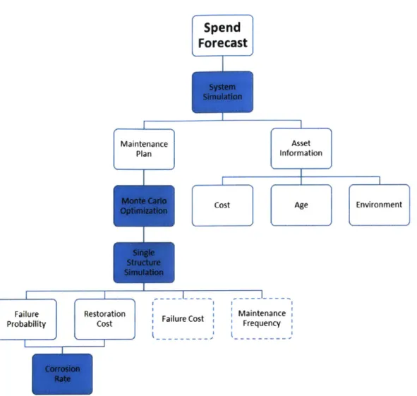
Figure 4 illustrates the forecasting flow. Shaded boxes in the figure represent simulation steps, while unshaded boxes are simulation inputs. Boxes with a dashed outline are inputs that were determined through optimization or were varied for scenario planning.

Spend

Forecast

MoteCaloCost Age Environment

Single Structure

Simulation

Failure Restoration Failure Cost Maintenance

Probability Cost Frequency

corrosion Rate

Figure 4: Forecast Flow

3.2 Corrosion Modeling

3.2.1

General Corrosion Background

Corrosion can be defined as the destructive attack of a metal by its reaction with the environment

[13]. This process is an electrochemical process by which anodic and cathodic reactions occur in a

coupled manner at different places on a metal's surface. This chemical reaction is therefore the sum

of the two half-cell reactions, which for steel can be written as follows:

At the local anodes: Fe -4 Fe2+ + 2e- (1)

At the local cathodes: 2H+ + 2e- -

(2)

The focus of this work is on atmospheric corrosion, which occurs in outdoor atmospheres due to the presence of thin film electrolytes formed on the metal surface. The rate of the metal dissolution process is strongly influenced by both endogenous factors, related to the metal itself, as well as exogenous factor related to the atmospheric composition, including humidity and the concentration of contaminants such as sulfur dioxide and chlorides [14].

3.2.2 Corrosion Calculation Methodologies

3.2.2.1 Overview of Methodologies

A number of efforts have been undertaken to develop methods for calculating the material loss of metals due to corrosion as a function of age and environment. These models can be classified as first level and second level models. First level models are based on physical laws, whereby the dissolution of metal and the formation of corrosion products are evaluated at a microscopic level. Second level models are based on fitting parameters to corrosion rate data collected through observation or experimentation [14]. Second level are generally used for structural engineering applications as they allow for macro-level predictions about the impact of corrosion over longer time periods.

Most corrosion models describe the corrosion depth as a function of time in a power model, as the formation of corrosion products on a metal's surface causes a decrease in corrosion rate over time. A general formulation of this model is shown in equation 4.

d(t) = A * tB (4)

Where:

d(t) is the corrosion depth t is the exposure time

A is the corrosion rate in period 1

B is the corrosion rate long term decrease

Examples of second level corrosion models include those created by the International Standard Organization [15], the European Committee for Standardization [16], Albrect and Hall [17], the International Cooperative Programme [18], and Klinesmith [19]. Landolfo compares these models, and illustrates the range of predicted section loss over time for the various models considered [14]. These plots are reproduced in Figure 5.

--- -AC pnhwwee ....I- hl e -.. - CP Vhetersd ₁₀ SO -50 0 1 2 3 4 5 0 5 10 15 20 nyi mu frers)

Figure 5: Landolfo's Comparison of Corrosion Model Predictions for Five and Twenty Years

3.2.2.2 ISO Corrosion Model

The simulation constructed for this analysis is based upon the methodology presented in ISO standards 9223-9226.

The ISO framework was chosen for its transparency, simplicity, and the industry credibility of the underlying organization. These standards also provide both qualitative and quantitative means for corrosion environment classification, which allows them to be combined with PG&E's internal corrosion zone classifications.

The general form of the atmospheric corrosion attack, and subsequently corrosion rate, is given in ISO 9224 as [15]: D = rcorr tb (5)

dD

(6)

t is the exposure time, expressed in years;

rcorr is the corrosion rate experienced in the first year expressed in micrometers per year; b is the metal-environment-specific time exponent

In the ISO standards, like other second level models, atmospheric corrosion rates are estimated to progress with exponential decay, as the corrosion layer inhibits further corrosion. The impact of this effect however is found to no longer provide additional protection after a sufficient coating of

- ISO 9224

-- - -EN 12500

1 -- ISO 9224 - - -- EN 125%4

corroded material is built up, after which point the material loss proceeds linearly. The ISO standards estimate this time to linearity as 20 years, reflected in equation 7.

3.2.3 ISO Model Implementation

3.2.3.1 Initial Corrosion Rate Determination

ISO 9223 provides multiple methodologies for determining the initial rate of corrosion, expressed in ISO 9224 as rcorr. The two primary methods are via a dose response function that takes as inputs environmental parameters, and a method that uses qualitative environmental characteristics to estimate an initial rate of corrosion. The direct dose-response calculation incorporates

environmental measurements of sulfur dioxide dry deposition rate, chloride dry deposition rate, temperature, and relative humidity into material specific equations for initial corrosion rate [20]. The equations are calculated by fitting coefficients of the dose-response function based on worldwide corrosion field exposure tests in addition to location specific pollutant and climactic data. For steel the resulting initial rate is expressed as follows:

rcorr = 1.77 *p0.s2 * exp(0.020 * RH + fst) + 0.102 * SO.62 * exp(0.033 * RH + 0.040 * T) (8)

fst = 0.150 * (T - 10) when T 5 10'C; otherwise - 0.054 * (T - 10) (9)

where:

rcorr is first-year corrosion rate of metal, expressed in micrometers per year T is the annual average temperatures, expressed in degrees Celsius RH _{is the annual average relative humidity, expressed as a percentage}

Pd is the annual average SO2 deposition, expressed in milligrams per square meter per day

Sd _{is the annual average Cl- deposition, expressed in milligrams per square meter per day}

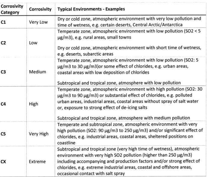
Because specific pollutant measurements were not available for PG&E's service territory, the dose-response equation estimation of initial corrosion rate was not utilized for this work; however ISO 9223 also provides numerical values for the first-year corrosion rates for standard metals based on qualitative corrosion categories. These categories range from C1 (very low) to CX (extreme). The description of these environments is shown in Table 2 [20].

Table 2: ISO 9223 Corrosion Categories

Corrosivity

Category Corrosivity Typical Environments - Examples

Dry or cold zone, atmospheric environment with very low pollution and

Cl Very Low _{time of wetness, e.g. certain deserts, Central Arctic/Antarctica}

Temperate zone, atmospheric environment with low pollution (S02 < 5

pg/m3), e.g. rural areas, small towns

C2

Low

Dry or cold zone, atmospheric environment with short time of wetness,

e.g. deserts, subarctic areas

Temperate zone, atmospheric environment with low pollution (S02: 5

pg/m3 to 30 pg/m3)or some effect of chlorides, e.g. urban areas,

C3 Medium coastal areas with low deposition of chlorides

Subtropical and tropical zone, atmosphere with low pollution

Temperate zone, atmospheric environment with high pollution (S02: 30

pg/m3 to 90 ptg/m3) or substantial effect of chlorides, e.g. polluted

C4 High urban areas, industrial areas, coastal areas without spray of salt water

or, exposure to strong effect of de-icing salts

Subtropical and tropical zone, atmosphere with medium pollution

Temperate and subtropical zone, atmospheric environment with very

high pollution (S02: 90 ig/m3 to 250 pg/m3) and/or significant effect of CS Very High chlorides, e.g. industrial areas, coastal areas, sheltered positions on

coastline____

Subtropical and tropical zone (very high time of wetness), atmospheric environment with very high S02 pollution (higher than 250 pg/m3)

CX Extreme including accompanying and production factors and/or strong effect of chlorides, e.g. extreme industrial areas, coastal and offshore areas, occasional contact with salt spray

The ISO standards additionally provide the following initial corrosion rate guidelines, in micrometers per year, as a function of corrosion zone [20].

Table 3: ISO Corrosion Rates in

sm/yr

Corrosivity Category Carbon Steel Zinc

C1 rcorr s 1.3 rcorr 5 0.1 C2 1.3 < rcorr 25 0.1 < rcorr 0.6 C3 25 < rcorr 50 0.6 < rorr 1.3 C4 50 < rcorr s 80 1.3 < rorr 2.8

C5

For this work, the ranges provided for each corrosion zone were translated into a normal

distribution with the high and low bound of the range each assumed to be two standard deviations from the mean rate.

3.2.3.2 Corrosion Rate Temporal Correlation

The model is structured in such a manner that the corrosion rate from one time period to another is correlated, therefore a structure that has an initial rate at the high end of its given corrosion level distribution will continue to age at this accelerated pace throughout its lifetime. Additionally, the corrosion rates for zinc and steel are taken from the same point in their relative distributions. If the rate between time periods were each selected independently, than the average rate of corrosion after a period of many years would revert to the mean for each structure evaluated, thereby reducing the variation in section loss from structure to structure.

3.2.4 Structure Properties

PGE&E design specifications for a standard lattice tower call for a structural steel member

thickness of 5000 um, or approximately 3/16" in accordance with PG&E design specifications [21]. Furthermore, these specifications call for steel to be galvanized in accordance with ASTM A123, which results in a zinc coating layer of 75 um [22]. While some towers and tower components may vary from these parameters, this standard was used across all steel structures in this analysis. This allows for a baseline aggregate forecast, however when considering any single structure, the specific properties of that asset should be considered.

3.2.5 Corrosion Model Output

By applying the ISO corrosion methodology to steel structures, a range of section loss over time can be calculated for each corrosion zone. The section loss is defined as a percent of the total member thickness, including the galvanized layer. The range in section losses within a corrosion zone is due to the range of possible starting corrosion rates as defined in the section above.

The resulting section loss over time for each zone is shown in Figure 6 with the lightly shaded area indicating the full range of outcomes and the darker shaded region highlighting cases within one standard deviation of the average, shown by the solid line.

0 0 100- 75- 5 0-0 50 Corrosin Zone CZ6 -..- CZ6 100 150 200 yewr

Figure 6: Section Loss over Time

The shape of these curves is due to two primary factors. There is a small, and barely visible, range

of accelerated section loss due to the exponential initial corrosion rate prior to the corrosion layer

inhibiting additional deterioration of the structure and entering the linear range of decay. The more

visible elbow that occurs in each range is due to transition from the zinc galvanized layer to the

steel layer which corrodes at a faster rate. Here the efficacy of a galvanized coating in slowing

overall corrosion can clearly be seen.

3.3 Single Structure Simulation

3.3.1

Failure Likelihood Estimation

In order to simulate the life cycle of a steel structure, the failure point of these structures must be

estimated. Because towers have not failed regularly in the field, no observed mean time to failure

statistics exist; however the design standards for towers can be used in order to estimate when the

structures would be at risk for such failures. In this work, a distribution of the failure probability of

a tower was created as a function of material section loss.

The IEEE National Electric Safety Code establishes a load factor requirement of 1.5 for vertical loads

in addition to transverse-wind and dead-end loads require safety factors of 2.5 and 1.65

Table 4: IEEE Transmission Structure Load Factors for Construction Grade B

Load Factor

Vertical Loads 1.50

Transverse Loads - Wind 2.50

Transverse Loads - Wire Tension 1.65

Longitudinal Loads - In general 1.10

Longitudinal Loads - At deadends 1.65

Given these load factors, the average failure was estimated to occur at a section loss of 33%, the

point at which the vertical load factor would be exceeded. A normal distribution with respect to

section loss was used to model failures, and a standard deviation of 10%. This results in an estimate

that only 2% of towers fail before the reach a section loss of 13% and only 2% of towers can last

beyond a 53% section loss before failure. A plot of the cumulative distribution function for tower

failures as a function of section loss is shown in Figure 7.

1.00 - 0.75-e 0.50-2 0.25- 0.00-0.0 0.5 050 0.75 10 Section Loss %

Figure 7: Tower Failure Distribution

3.3.2

Modeling Life Cycle Events

Similar to the work performed by Transpower, maintenance events are assumed to be able to

restore the life of the tower through the replacement or treating of the most heavily corroded

elements of the tower, thereby reducing the average section loss of the tower, as well as

temporarily prevent future section loss through the application of a coating.

A maintenance event is assumed to restore the asset to a maximum average section loss of 5%, and as specified by the National Association of Corrosion Engineers, the application of a coating is assumed to prevent additional section loss for 5 to 12 years, depending on the corrosion zone of the asset [24].

3.3.3 Cost Estimates

The benchmark cost estimates used for this analysis were derived by previous work performed by PG&E. In that work, replacement costs for a variety of steel structure types was assembled, and an estimate of $35,000 per structure for coating was developed.

This analysis maintains the replacement costs used in that analysis, and uses the $35,000 coating cost as an upper bound, with the lower bound being set at 10% of the tower replacement cost. An adjustment factor of 10x was also included for structures located on a body of water, given the increased costs associated with these jobs.

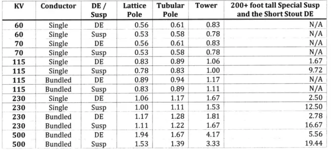
The cost of failure is also considered in this analysis. This cost is intended to include not only the structure replacement, but any associated externalities including customer outages, emergency response, damaged property, loss of reputation, and any other additional costs. The average cost of failure was assumed to be 10x the replacement cost. In future work this cost can be refined on a structure by structure basis as a function of several factors including customers served by the line, system stability parameters, population safety risk, fire risk, and any additional safety hazards. Table 5: Tower Cost Index -Normalized to 115 KV Suspension Tower

KV Conductor DE / Lattice Tubular Tower 200+ foot tall Special Susp

Susp Pole Pole and the Short Stout DE

60 Single DE 0.56 0.61 0.83 N/A

60 Single Susp 0.53 0.58 0.78 N/A

70 Single DE 0.56 0.61 0.83 N/A

70 Single Susp 0.53 0.58 0.78 N/A

115 Single DE 0.83 0.89 1.06 1.67

115 Single Susp 0.78 0.83 1.00 9.72

115 Bundled DE 0.89 0.94 1.17 N/A

115 Bundled Susp 0.83 0.89 1.11 N/A

230 Single DE 1.06 1.17 1.67 2.50 230 __Single Susp 1.00 1.11 1.53 12.50 230 Bundled DE 1.17 1.28 1.81 2.78 Bundled Susp 1.11 1.22 1.67 16.67 500 Bundled DE 1.94 1.671 4.17 5.56 500 Bundled Susp 1.53 1.39 3.33 19.44

Consistent with methodology established by Transpower, the cost of maintenance was assumed to

be a function of the degradation of the asset. Because the simulation assumes that any maintenance

activity restores the tower to the same condition, the cost becomes the dependent variable in the

relationship between maintenance timing, asset condition, and cost.

The cost was modeled with a floor of the coating cost

-

defined as the smaller of 10% of the

replacement cost and $35,000

-

and a ceiling of the replacement cost. A logarithmic function was

created to return this range of values over the range of section losses consistent with the expected

section losses that could be seen in the field prior to failure. An example of this curve for a structure

with a $100,000 replacement cost is illustrated in Figure 8.

100- 75- 50- 25-0.0 0.1 0. 0.'3 0.4 0.5 Section Loss % Figure 8: Tower Maintenance Cost Curve

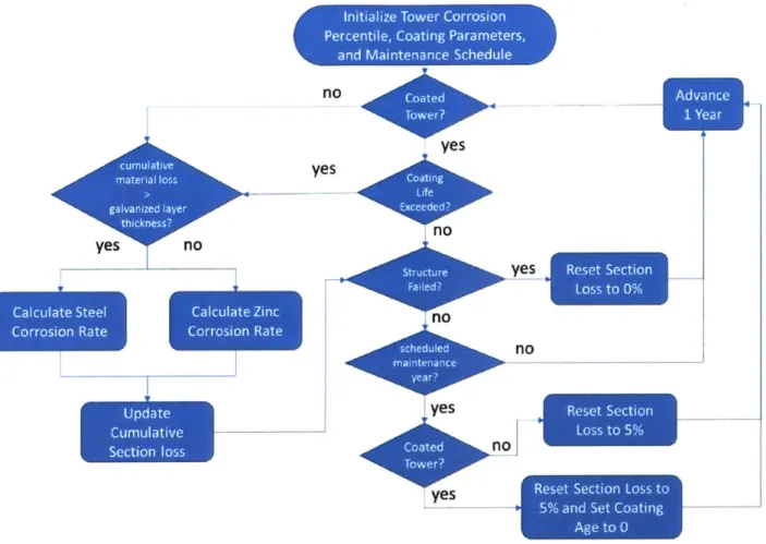
3.3.4 Tower Life Cycle Simulation

The life cycle of a single tower can be simulated by applying the corrosion aging equations together

with the failure probabilities and an assumed maintenance schedule. As the simulation iterates over

each year, some amount of section loss occurs as a function of the corrosion rate distribution and

the material being exposed

-

steel, zinc, or coating. Each iteration through the simulation the

structure also experiences some probability of failure as a function of its state of section loss.

Maintenance and coating occurs on a predetermined cadence, resetting the section loss of the tower

to the 5% threshold, and preventing the corrosion of the underlying structure for the life of the

coating. A diagram of this simulation is shown in Figure 9.

no

yes

yes

yes

EmL

Ya

no

no

yes Reset Section

5% and Set Coating Age to 0

Figure 9: Tower Aging Simulation Flow Diagram

As example of the results of this simulation for a tower in a severe corrosion zone with coating and

maintenance occurring every 30 years is shown in Figure 10. As can be seen the simulation applies

the corrosion rate associate with zinc until approximately 3% section loss occurs. Beyond this

point, the simulation uses the corrosion rate of the underlying steel, and an acceleration in the

corrosion rate occurs. 30 years after the galvanized layer has been corroded away, the tower goes

through a maintenance cycle, which restores the structure to a 5% material loss. The simulation

also applies a coating at this point, which lasts for approximately 6 years, after which point the steel

again begins to corrode. At just after year 90, a failure and subsequent replacement occur in the

simulation, after which point the aging cycle begins again.

yes

Steel

S-- Galvanized Layer Replacement

0 50 100

" Maintenance event

" Failure event

150

Tower Age

Figure 10: Example Tower Simulation

3.4 Maintenance and Replacement Optimization

In order to determine an appropriate maintenance schedule for calculating total system spend, an

optimal maintenance and replacement cadence for transmission structures was calculated.

The optimization is formulated in equations 10 and 11, where the goal is to minimize the present

value of all cash flows associated with failures or repairs, where in this case replacements qualify as

a subset of repairs.

Objective Function:

Present Value Calculation:

min>

t=o

FtCf + RtCR

~t

Where:

Rt: Binary decision variable with value 1 if repairs occurring at time t, 0 if not

PVt: Present Value of costs at time t

Ft: Probability of failure at time t given section loss at time t

Cr: Cost of failure

CR:

Cost of repairs at time t given section loss at time t

r: Discount Rate

No closed form solution exists for this system, and as a result the optimal maintenance and

replacement cadence could not be calculated directly. Instead, the lowest cost maintenance

schedule was identified through a Monte Carlo simulation. In this analysis, 10,000 trials were

0 -J V,-0

-(10)

(11)

performed under each set of maintenance parameters

-

including the timing of initial maintenance

and the frequency of maintenance thereafter

-

and at each corrosion zone.

In each of these simulations the cost of each maintenance event, as well as any failures that may

occur were tracked, and summed in accordance with a discounted cash follow equation using a

7% discount rate applied. The average was then calculated for the 10,000 runs under each set of

conditions. Figure 11 shows the result of each of these calculations over the ranges of parameters

considered.

Corroion Zne 4 Coding Frequency

40 50

Coroe on Zone 4

5000-

13000-0 10 20 30 Q 50 Ciur Fren nic

Figure 11: Maintenance Plan Discounted Costs

Sat 30 SMt40 Sab"100 Corosion Zone 5 15000- 1500- 5000-0 10 20 30 40 50 Codng Frequency Corrosion Zone 3 50-0 10 20 30 40 50 Cofing Frequency

The analysis demonstrates that in more aggressive corrosion environments, a more frequent

coating schedule leads to a lower total cost. This is because in these faster aging environments, the

probability of failure, and the associated cost, increases more rapidly than in less corrosive

environments, and as such investing in preventative measures becomes worthwhile. For assets in

lower corrosion zones the optimal maintenance strategy is to wait several decades before

beginning maintenance, and then only to perform occasional preventative maintenance. This

.

further illustrates that the optimal maintenance schedule balances the tradeoff between cost due to structure failures and costs associated with preventative maintenance.

The lowest cost scenario for each corrosion zone is shown Figure 12. In low corrosion

environments, an optimal maintenance strategy does not require maintenance until 40 years after the structure first loses its galvanized layer, and only every 30 years after that point. In a highly corrosive environment, however, maintenance may be required in the first year after the

galvanized layer is lost and as frequently as every 6 years after that point. To illustrate the necessity for more frequent maintenance for structures in a more aggressive corrosion zone, an image of a tower structure located in the San Francisco Bay, taken 5 years after maintenance activity is shown in Figure 13. 40 30 30 20 14 10 6 0 ₆₁ CZ3 CZ4 CZ5 CZ6

U First Maintenance E Maintenance Cadence

Figure 13: Tower in Corrosion Zone 6 after 5 years

3.5 System Simulation

3.5.1 System Simulation Inputs

In order to perform an aging simulation across the system simulation, each structure must be given initial conditions based upon its location and age, and a maintenance schedule must be applied. Maintenance schedules in accordance with the asset's corrosion zone and the analysis performed in the previous section were used.

3.5.1.1 Corrosion Zone Assignment

Based on the location of the structure, the structure is classified into one of four corrosion zones defined by ISO 9223. These metrics were simplified in order to maximize model transparency by taking advantage of the internal PG&E corrosion zone maps which had been produced the

In order to classify each asset into one of these six categories, the following heuristic was employed.

All structures were placed into a category of C3 at a minimum to help ensure a conservative

estimation of degradation.

Table 6: Corrosion Level Classification Heuristic

Corrosion Level

Parameter

CX

In San Francisco Bay

C5

On water OR in PG&E severe corrosion zone OR near coast

C4

In moderate PG&E corrosion zone

C3

All others

Results of this classification are displayed in Figure 15.

1 0 0 I 6 4

Pp 0s

1 24

Wan

s$er0 Croewn Am*

Modee COnIeMn Aa

Corosion Zone

CZ4

+

Z5

x CZ6

Figure 15: Assets by Corrosion Zone

3.5.1.2 AssetAge

Asset age was determined from internal PG&E records that indicate the installation year for each transmission line. Assets with no given installation date were removed from the dataset for the aging simulation, resulting in the inclusion of 38,997 of the 48,061 total records.

A histogram of the installation history of PG&E's steel transmission structures is shown in Figure 16, where the dominance of post-war construction, particularly of the high voltage system is evident.

9

4000-kV &60 *70 o -115

I

Figure 16: Structure Installation Year

3.5.2 Simulation Execution

The maintenance cadence for each asset, along with its corrosion zone, age, and costs, comprise the necessary initial conditions for a system-wide simulation. The simulation is executed beginning at a time prior to any towers being installed, in this case 1900 was used, and as each structure's

installation year arrives, that structure begins to age in accordance with the ISO guidelines. As the simulation iterates forward in time, the cost of each maintenance and failure event is tracked. If a maintenance event occurs and over 95% of the structure's replacement cost is necessary, this event is classified as a replacement.

Given that no systemic preventative maintenance plan has been put into place to date, no maintenance activities are assumed to begin until the current year, 2018.

3.5.3 Spend Forecast

3.5.3.1 Cost Events

The cost events resulting from the system simulation, including the application of the optimized maintenance schedules, by corrosion zone, are shows in Figure 17. These results have been

smoothed over a 10 year period in accordance with the assumption that maintenance schedules can be smoothed to some degree over this period. The insert to the left zooms in on the estimated

number of failures and replacements, which are significantly fewer than the estimated number of repairs.

1 20-I 1 1 2000- 15-W''A 10- 10 5-2040 2070 21100 2040 2070 Yew Yew 006 Rpas_.SonouMed Faikurs..Smoeowd 2100O

Figure 17: Asset Cost Events

In this optimized plan all replacements occur in the early years, and are a result of replacing a

backlog of high risk towers. In future years, the plan is dominated by preventative maintenance.

While this plan calls for no replacements, other than those towers which have already endured

excessive aging prior to the implementation of the optimized maintenance schedule, some

conditions may arise which would call for additional replacements. For instance, the

implementation of a just-in-time replacement strategy that occurs later in the life of a structure may

be possible if the variance in the distribution of expected tower lifetime is narrowed due to:

* More precise estimation of failure point as a function of section loss

" More precise predictions of corrosion rates

* Or the implementation of inspection procedures that able to provide more complete

information regarding asset likelihood of failure.

Additionally, if preventative maintenance is unable to restore tower health as much as assumed in

this work and the work of Transpower, than the trade-off of replacement versus repair may

advantage replacing structures under some conditions.

3.5.3.2

Total Cost Projection

The associated cost projection associated with the events from Figure 17 is shown in Figure 18.

While working through the backlog of accumulated maintenance resulting from prior

levels dropping to approximately one third of the starting levels, after which point spend slowly

escalates as the system continues to age, and preventative maintenance needs increase.

RunuAe

Repnir*_9mo u0W

Faibxur.._SmocUhed

2040 2070 2100

Ye-Figure 18: Cost Projection by Event Type

3.5.3.3 Cost Projection by Corrosion Zone

The system spend estimation can also be viewed by corrosion zone, as shown in Figure 19. Assets in corrosion zone 6, largely composed of the towers located in San Francisco Bay, have an outsized effect on the spend forecast as they undergo accelerated corrosion and are significantly more costly to repair or replace as they are built on water. These structures are anticipated to need significant

maintenance and replacement work over the coming decade, and in then they will require ongoing preventative maintenance in perpetuity to prevent an increasing likelihood of failure.

A ramp up in spend for the lower corrosion towers that make up the majority of the system occurs after 2050.

2040 2070 2100

Figure 19: Cost Projection by Corrosion Zone

3.5.3.4

Cost of Failure Sensitivity

Figure 17 shows that in this cost optimized plan, some number of structure failures are still

estimated, reaching a level of approximately 5 per year in year 2100 and beyond. Adjusting the

maintenance schedule to reduce spend associated with failures is possible; however doing so would

implicitly increase the cost of failure, as this would result in a higher spend to avoid these failures.

To illustrate this a sensitivity analysis was performed by adjusting the cost of failure from a

multiple of 2x the replacement cost, to 100x the replacement cost, and optimizing the maintenance

cadence in each zone accordingly. This maintenance reoptimization lead to more frequent

maintenance events as a higher cost of failure leads to a greater sensitivity to failure and therefore

increases the optimal level of prevention. Section 4 of this thesis will more rigorously demonstrate

this balance.

As can be seen in Figure 20 and Figure 21 higher failure costs lead to a schedule with more

maintenance and fewer failures, while lower failure costs lead to an optimal strategy of running to failure. This eliminates maintenance for lower corrosion zone towers, but resulting in increasing

50- 40- 30-IL 0 U 20- 1 0-2040 2070 Year . ~j 2100

Figure 20: Asset Failures over Time by Failure Cost Factor

2000 -LO 0. aL 1000. 2040 2070 - Repai2 ... RepairO --- Repair2 - - - Rpair0O 2100 Year

Figure 21: Repairs over Time by Failure Cost Factor

The impact on net present value for each of these plans as a function of the baseline assumption of a

10x failure cost multiple are shown in Figure 22. As expected, plans burdened by a higher failure

cost result in a higher NPV, but by reoptimizing the maintenance plan under each condition, the

impact of these additional costs are mitigated.

-Fallures2 Failures1O --- FaIlures20 - - Failures100 't- -0.

160% 140% 120% Z 100% 80% 60% 40% 20% 0% 0 20 40 60 80 100 120

Failure Multiple (x Replacement Cost)

Figure 22: Optimized System NPV Costs as a Function of Failure Multiple

3.6 Conclusions

A spend forecast for the ongoing operation of the steel transmission structure fleet, optimized for

cost, was developed by combining estimates of atmospheric corrosion rate, structural properties,

repair costs, failure costs, and maintenance scheduling. This integrated approach allows for the

development of an aggregate forecast, and enables sensitivity analysis on the underlying factors.

Through this forecasting the following conclusions were reached:

" An NPV optimized maintenance strategy includes more frequent maintenance activities for

structures in more aggressive corrosion zones, while structures in less aggressive

environments require maintenance at a significantly lower cadence.

* For aging systems with no history of regular preventative maintenance, replacement of

older structures in high corrosion zones may be necessary in the near term, after which

point the optimized maintenance schedule should be applied.

* Given the level of uncertainty regarding tower life expectancy, due to the underlying

uncertainty in the distributions of both corrosion rate and failure point, a strategy of

preventative maintenance has lower overall costs than a replacement strategy. If data

collected in the future allows for a true just-in-time replacement option, then this may no

longer be the case; however under current conditions the elevated expected cost of failure

for an aging tower due to uncertainty around failure estimates does not warrant this approach.

* The lowest NPV strategy of preventative maintenance will likely rely heavily on an increase of expense dollars as opposed to capital dollars. While like any business, utilities should be seeking to lower their overall costs, this accounting tradeoff may require additional

discussions with regulators in order to align the interests of all stakeholders, given that currently utilities are generally remunerated through a return on assets mechanism.