Determining shape and reflectance using multiple images

(1)

Determining Shape and Reflectance

Using Multiple Images

by

William Michael Silver

B.S., Massachusetts Institute ofTcchnology (1975)

Submitted in Partial Fulfillment of

me

Requirements for the

Degree of

Master of Science

at the

Massachusetts Institute of Technology June

1980

__..--;

-Signature redacted

Signature of Author _ _

~=, ~ ~ ~

-Dcp,1rtmcnt of Electrical Engineering :ind Computer Science

Signature redacted

tv1ay 9, i980 Certified b Y = = = = = 1 = = = -Accepted by _ _ _ _ _

ARCHIVES.

U (") [ \ '. () . '- ·1...:i _I..J _I _f..• C:• 1Q A • ...JV' UBRAR!ES Berthold K. P. Horn Thesis Supervisor

(2)

Determining Shape and Reflectance

Using Multiple Images

by

William Michael Silver

Submitted to the Department of Electrical Engineering and Computer Science on May 9, 1980 in partial fulfiliment

of the requirements for the Degree of Master of Science in

Electrical Engineering and Computer Science

ABSTRACT

This thesis is an investigation of photometric stereo, a practical technique for determining an object's shape and surface reflectance properties at a distance. It makes use of multiple images of a scene, recorded from the same viewpoint but with different illumination. It is a photometric technique because it makes direct use of the irradiance measurements recorded in an image to provide constraints on dic possible interpretations that can be assigned to a given surface element. Output is in the form of an array of surface normal vectors and a small number (0, 1, or 2) of arrays of surface reflectance parameters, all registered with the original image arrays. The &alculation itself, after an initial calibration step, is purely local and may be implemented by table lookup, allowing real-time performance. Possible applications include industrial automation, analysis of planetary explorer images, and other situations where the ilUmination can be controlled or at least measured.

The research is divided into two components, one theoretical and the other experimental. The pioneering work of Woodham is presented and extended to handle certain types of non-uniform surface cover. Two models of non-uni form surfaces are investigated. The simplest combines a known reflectance function with an unknown multiplicative reflectance factor, called Ute albedo. The more sophisticated allows, in addition to the albedo, an unknown mixture of two known reflectance functions, for example a matte and a specular component.

The experimental part of this research is a detailed quantitative evaluation of a working implementa-tion of photometric stereo. The purpose of the experiment is not only to show how well such a system can

be expected to work, bUt also to give specific algorithms and procedures that can be used to reduce the

theory to practice.

Thesis Supervisor: Professor Berthold K. P. Iorn

Title: Asscolate Professor of Computer Science and Engineering

(3)

Ac know ledgements

I would like to thank my thesis supervisor, Professor Berthold Horn, for suggesting this research topic, for

his continued support and enthusiasm throughout this lengthy effort, and for many valuable suggestions

for and criticisms of this material.

This research would not have been possible without the facilities and environment provided by the

M.I.T. Artificial Intelligence Laboratory. The skills of many people of diverse interests combine to make

this unique and stimulating atmosphere. For this I am gratefil to professors, engineers, students and

hackers too numerous to mention.

I owe a great deal to my parents, Edward and Barbara, for encouraging ine to persue those activities

that I enjoy, for considerable financial support, and for a large dose of good judgement, understanding,

and love throughout my life.

Finally, a special note of gratitude to Barbara-Joan, for being there all the time, for being slightly

crazy, and for never letting me forget that there are other things in life besides computers.

(4)

6

Table of Contents

(7)

List of

Figures

2.1. Definition of Viewing Geometry 22

2.2. Beam Geometry for Specifying Reflectance 27

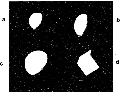
4.1. The Objects Used in the Experiment. 46

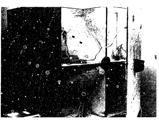
4.2. The Plywood "Studio" 47

4.3. A Typical Scene Photographed in the Plywood Box 48

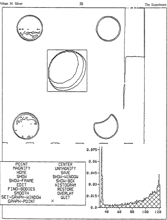
4.4. The Lisp Machine in Use 50

5.1. Relief Plot of the Egg 66

5.2. Relief Plot of the Knob 67

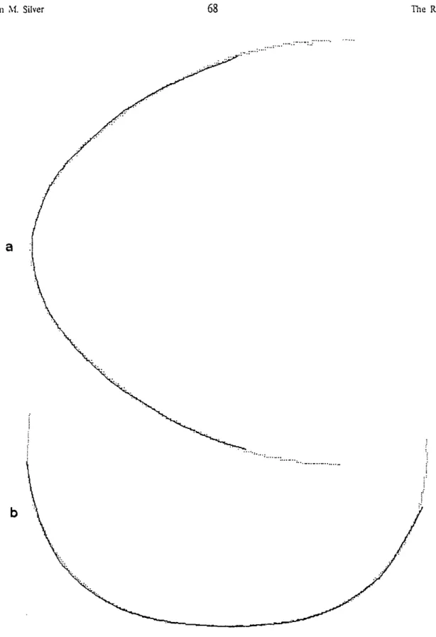
5.3. Egg and Knob Profile Comparisons 68

5.4. Error Regions Produced by the Reflectance Maps 69

5.5. The Angular Error Statistics 71

5.6. Distance Distribution for the Egg and Knob 70

5.7. Statistics of the Integral of Gradient Around a Unit Pixel 73

5.8. Angular Error Distributions for Different Table Sizes 74

5.9. Mean Angular Error vs. Table Size 72

5.10. Relief Plot of Egg using Small Table 76

5.11. Egg Profile Comparison using Small Table 77

5.12. 1)istribution of g, from the Sphere for Different Table Sizes 78

5.13. Angular Error vs. View Angle for Different Intensity Biases. . 80

(8)

William M. Silver

5.14. Mean Angular Error vs. Intensity Bias 79

5.15. Error Regions with Optimal Intensity Bias 81

5.16. Angular Error Distributions for Different Table Sizes with Interpolation 83

5.17. Mean Angular Error vs. Table Size, with Interpoaltion 84

5.18. Relief Plot of Egg using Small Table with Interpolation 85

5.19. Egg Profile Comparison using Small Table with Interpolation 86

5.20. Distribution of g from the Sphere for Different Table Sizes with Interpolation 87

5.21. Relief Plot of Pyramid 88

5.22. One View of the Pyramid 89

5.23. The Smoothness Functions gi Applied to the Pyramid 90

(9)

CHAPTER 1 INTRODUCTION

This thesis is an investigation of a practical technique for determining an object's shape at a distance.

The investigation has both a theoretical and an experimental component. On the one hand, methods for

extending the range of surfaces for which the technique may be applied are developed. On the other,

construction and detailed quantitative analysis of a working implementation add weight to the use of the

term, "practical".

The methods presented herein are a natural result of a photometric approach to certain aspects of

machine vision. The central observation of this approach is that:

grey-levels recorded by an imaging device are measurements which result from real physical

processes. Such a measurement may be viewed as a constraint on the possible interpretation

of the surface element that gave rise to it.

A detailed understanding of the physical processes underlying image formation has led to methods for

determining object shape and, to a limited extent, surefCe material, by making direct use of the grey-levels

recorded in an image.

(10)

Wiffiain M. Silver

Photometric techniques may be applied when imaging variables, such as illumination and viewing

geometry, can be controlled or at least are known. Examples include many problems in industrial

automa-tion, where a designer may be free to set tip conditions necessary to achieve a desired result, and analysis

of images recorded by planetary explorers, where the positions of the sun and camera may be precisely

determined. The approach is of little value for the unconstrained vision problems facing, flor example, a

mobile, self-supporting robot or biological entity.

The methods explored here all make use of multiple images of a scene, taken from die same

view-point but with varying illumination. The basic idea, called photometric stereo, was first described in

[Woodham 1978], and represents a major advance in the photometric approach. In situations where the

necessary images can be obtained, photometric stereo avoids many of the serious problems associated with

previous techniques. In addition, it is probably the least comiputationally expensive method available for

determining object shape. Implementations on present-day minicomputers would be quite capable of

real-time performance. Special-purpose hardware could conceivably run at video rates.

Virtually all of the fundamental ideas which form die basis of this research were initially developed

by others. '[he contribution of this work, if any, lies in the attempt to extend the usefulness of these ideas,

and the presentation, for the first time, of a thorough analysis of a working system.

1.1 Machine Vision-The Problem

Vision, artificial or natural, may be defined as a process whereby object properties relevant to a

particular application are determined by an analysis of the spatial, spectral, and temporal distribution of electromagnetic energy radiated by those objects. (Let us immediately strike the spectral and temporal

components from further consideration.) Several factors combine to make that analysis both difficult and

cornputationally expensive.

First is the slicer quantity of information present. For example, a standard vidicon camera, which is

(11)

not considered a very high resolution device, could produce over 7 million measurements every second,

given an interface that could absorb data at that rate. With the basically serial hardware that is typically

available, evon the most elementary operations will be time consuming.

The second difficulty is that the physical quantity being measured, scene radiance, arises from the

interaction of several factors, some of which are properties of the objects being viewed and some of which

are not. The influences of those which are- shape and surface material-must be separated from each

other and from the influences of those which are not-illumination and viewing geometry.

Third, the transformation from the three-dimensional object space to the two-dimensional image

space introduces difficulties. Information is lost in such a mapping-a given image will typically have

many physical interpretations. Additional information must be brought to bear if we are to have any

hope of finding the "correct" interpretation. Often, additional information is obtained in the fori.. of

multiple images (this work is an example). By far the most important, if not universally accepted, source

of additional information, however, is prior expecatlion. In this work, for example, prior knowledge is

represented by a function called the reflectance map, which incorporates information about illumination,

viewing geometry, and surface photometry. Previous researchers in machine vision often made explicit use

of the fact that their images were of scenes containing only plane-faced polyhedra [G uzman 19681, [Waltz

1975]. In human vision, the influence of prior expectation pervades virtually all stages of visual processing.

The proper use of prior expectation is difficult. A balance must be struck between using so little

that one's methods apply to any situation but yield little information, and relying on so much that they

would tell one everything if only they applied to the situation at hand (this work tends towards the latter

extreme). In addition, a system should be capable of producing some resulIts even if its prior expectations

are not exactly met.

Loss of information is not the only problem caused by the transformation from object space to image

space. Features in an image may just be artifacts of the projection geometry, not related to any real object

(12)

William A. Silver

features. An example is an occlusion contour, which is a curve separating surface elements tilted towards

the viewer from those tilted away from the viewer.

The final difficulty we note here is that the properties of interest in a particular situation may be so

far removed conceptually from the actual input data that many complex levels of description must be built

tip before such properties can be determined. A good example of such a property is the identity of a

human face. Somehow, a human can quickly and without apparent effort extract a friend's name from

what is essentially a two-dimensional array of numbers produced by his retina. Most of the intermediate

steps are quite beyond our understanding. What is clear, however, is that these issues of description and

representation are among the most important, and difflicult, of the problems in vision research (see, for

example, [Marr 1978]).

1.2 Approaches to Early Visual Processing

This work is concerned with the earliest level of visual processing-that level which has as its input

the raw irradiance values recorded in an image. It is expected that a system built along the lines described

here would be incorporated into a larger system designed to satisfy some higher-level needs.

There is a basic philosophy behind our approach to early vision. To help appreciate this philosophy,

we will compare it to others that have appeared in the machine vision community.

1.2.1 Classical Image Analysis

Much of the classic research in machine vision was concerned with the interpretation of scenes

con-taining plane-faced polyhedra (often called the "blocks-world"). Researchers divided the vision problem

into two sub-problems. with (initially) a wel!-defined bO ndlary-inlage analysis and scene analysis.

Simply stated, the purpose of image analysis is to take the raw grey-levels and produce a symbolic

descrip-tion of the scene by extracting image features (line-segments in the blocks-world) [Binford & I lorn 19731,

(13)

[Shirai 1975]. Scene analysis would then interpret this symbolic description in terms of goals dictated by

some specifc application.

It is very tempting to refer to the present work as an exercise in image analysis. It can also be very

misleading, for about the only similarity between classical image analysis and this work is that they both

have raw images as their input. The following are the major differences in approach:

Data Compression: An important result of classical image analysis is a great reduction in the amount

of information present. This was considered necessary to make the computational load on subsequent

scene analysis managable. Our method produces a local description of surface orientation and reflectance

at each data point in the original images. If anything, the amount of data has increased.

Symbolic Descriptions: A major goal of classical image analysis was dte generation of symbolic

descriptions, typically in the form of a line drawing. Her, we produce strictly numerical results-local

surface normal vectors in a viewer-ceatered coordinate system.

Image Features: Classical image analysis is concerned with finding 1eatures that are properties of the

image. As noted earlier, such features are often artifacts of the imaging process and bear no direct relation

to properties of the objects themselves. Thus, the symbolic descriptions passed up to the scene analysis

system still contain the combined effects of illumination, viewing geometry, surface material, and shape.

This significantly complicates subsequent analysis, because most of the intormation that could have been

used to separate these effects has been thrown away. In contrast, here the goal is to directly extract features

which are properties of the objects themselves. T'he results have the effects of illumination and viewing

geometry removed, and the effects of surface reflectance and shape appearing explicitly. ''his greatly

simplifies further analysis, because we are dealing with descriptions of objects rather than images.

To summarize: In classical image analysis, we extract those image'features that seem relevant, and

throw everything else away, yiciding a symbolic description of the image. Here, we try to use all of the

information contained in an image to produce a quantitative description of the objects that gave rise to the

(14)

image.

The above discussion should not be viewed as arguing that our methods are necessarily "better"

than previous ones, rather just that the approach is different. We require explicit prior knowledge of

illumination, viewpoint, and surface photometry before our techniques can be applied. Such knowledge

in often not available, and in such cases the more traditional approach to image analysis is really all we

can do. There are enough cases where the information is available, however, to justify developing the

photometric approach.

1.2.2 Marr's Approach to Early Visual Processing

Marr's school is concerned with the relatively unconstrained situations facing biological vision

sys-terns, where explicit knowledge of the imaging variables is not available. Since their goals and assumptions

are different from ours, it is diicult to compare the two approaches directly. Still, similarities between

the two approaches are evident from the representations that Marr has developed to explain early visual

processing [Marr 1976], [Marr 1978](recall the importance of representation, noted above).

Marr observes that the early symbolic representations used in vision should be influenced primarily

by what it is possible to compute, leaving what it is desirable to compute to later levels. Consequently,

his earliest representation, called the primal sketch, is a description of primitive features of a raw

hmage-intensity changes and local geometry. Marr shares our view (in contrast with classical image analysis) that as much information as possible should be extracted from an image before discarding it. In fact, Marr has

shown that the primal sketch contains most of the information present in the original image [Miarr 1978].

A program was written that could produce a reasonable r&construction of an image from its primal sketch.

The next level representation used by Marr is called the 2{-D sketch. It is a quantitative,

viewer-centered representation of object shape, which contains local numerical descriptions of surface orientation

and depth, along with contours of surface discontinuities. Although it is determined by totally difTerent

(15)

William M. Silver

means, it is virtually identical to the representation produced by photometric stereo.

1.3 Development of the Photometric Approach

The idea that the irradiance measurements recorded in an image can be used to determine object

shape is not new. The first such attempt was reported by van Diggelen in a 1951 paper concerned with

the hills in the Maria of the Moon [van Diggelen 1951]. These features were too small to be analyzed

by their cast shadows, the traditional method for determining the heights of features on the Moon. Van

Diggelen did not use the surface reflectance properties of the Maria, so his methods could be applied only

to small regions near the terminator1, where the view angle and the phase angle2 could be considered

constant. Interestingly, van Diggelen had the basic idea behind photometric stereo in his paper, but failed

to develop it. He rejected using two images taken with the sun in different positions, because a lunar

surface element could not be near the terminator in both images.

Although van Diggelen did not use them, the photometric properties of the Moon have been known

at least since 1929, when they were measured by [Fesenkov 1929]. Finally, [Rindfleisch 19661 showed

how these specific properties led to an exact solution for surface elevation from a single image. He

applied his method to images returned by the Ranger spacecraft, and speculated that there should be

other photometric properties which give rise to exact solutions.

Rindfleisch's speculations were confirmed when [Horn 1970J, showed how the shape-from-shading

problem could be solved for virtually any surface reflectance function (non-isotropic, and highly specular

surfaces still could not be handled). His method involved the somewhat tedious numerical solution of a

nonlinear first-order partial differential equation. The technique was demonstrated using a crude

imnage-dissector camera interfaced to a PDP-6 computer.

11110 boundary between the illuminated and the dark hemispheres.

2The angle between rays from a lunar surface element to the Earth and Sun.

(16)

William NI. Silver

[Woodham 19731 elaborated on Horn's results, by showing how assumed monotonicity relations,

such as convexity or concavity, could be used in conjunction with a single image to determine object

shape, without requiring Horn's numerical solution. More significantly, that report contained a description

of a new technique, photometric stereo, which could determine object shape from several images taken

from the same viewpoint but with different illumination. The new method is faster, more accurate, and

requires fewer assumptions than previous methods.

[Ikeuchi and Horn 1979] showed for die first time how photometric stereo could be applied to

per-fectly specular surfaces, by using specially designed extended light sources. The result is important in

many industrial settings, where highly specular metallic objects must be handled.

All of the above methods assume uniform surface material, probably their most significant limitation.

[Horn et al 1978] showed how to relax this assumption slightly, by allowing a multiplicative relectance

factor which varies across die surface. This work attempts to extend these ideas, by developing a more

complex model of the way a surface can be non-uniform (Chapter 3).

1.4 Overview of The Thesis

Chapter 1 introduces the thesis and illustrates its relationship with related research efforts. The work

is presented as a problem in early machine vision. Reasons why it is difficult to build seeing machines

are noted. Our approach to early vision is compared with others that have appeared. The historical

development of this appraoch is traced.

Chapter 2 presents the basic theory behind photometric shape-from-shading methods in general,

and photometric stereo in particular. We see that an individual irradiance measurement constrains the

orientation of die surfce element that gave rise to it, but not enough to uniquely determine it. '[he

various photometric niethods that have appeared may be characterized by die way in which they seek to

determine the additional constraint needed to find a unique solution. Before this can be done, however,

(17)

William A. Silver

concepts we have been using informally (such as shape) must be made precise, and relevant tools must be

developed (gradient space, the reflectance map). Since these ideas have been presented in at least a dozen

places, only the briefest attention will be given to them at the beginning of this chapter. For the benefit of

the uninitiated, a more thorough development is given in Appendix A.

Chapter 3 develops methods for dealing with non-uniform surface material. First the simple

"multiplicative reflectance factor" model is presented. The interesting simplification that occurs when

this model is applied to lambertian reflectors is discussed. Next, the "variable linear combination of two

reflectance functions" model is developed. Again, an interesting simplification occurs when one of the

reflectance functions is lambertian (although this case is much different than the first case). Finally, a promising technique is presented for dealing with situations when surface photometry is unknown and

cannot be measured directly.

Chapter 4 describes in detail the experiment that was perfonned-iks goals, the experimental setup,

and how the data were processed. Chapter 5 gives the results of the experiment. It includes many graphs

and charts, of both a qualitative and quantitative nature, showing the effects of various parameters that

were investigated. This information is then put into words, and its significance is discussed. Note: A casual

reader

just

interested in an overview of the expreiment and a summary of the results should read sections 4, 4.1, 4.2, 5, and 5.6, and ignore everything else in Chapters 4 and 5.

Chapter 6 presents a brief summary of the work along with some concluding remarks.

Appendix A gives the details of gradient space and ihe reflectance map promised in Chapter 2. It

also discusses the lambertian model of reflectance, which has been studied extensively and is necessary for Chapter 3. With the exception of the results on illumination of lambertian surfaces, all of this Appendix is

well known in the vision community and has been reported many times elsewhere.

Appendix B gives the details of a highly effective technique for automatically registering simple

profiles for shape comparison. The rotation, scale, and translation necessary to align two sinmilar profiles is

(18)

William M. Silver 18 Introduction

determined using best-fit conic sections. The method was used as part of the check on the performance of photometric stereo, as described in Chapters 4 and 5.

(19)

CHAPTER 2 SHAPE FROM SHADING

If we are to determine object shape from image irradiance, we must first have two things. One, we need

a precise definition of shape. As noted by Marr (see Section 1.2.2), such a definition will be motivated more by what it is possible to mCasure than what might be ultiiatly desirable. Thus we will end up with

a viewer-centered representation, rather than an objeci-cenaered representaion (which would simplify later

operations such as object identification). Shape will be defined as a collection of surface normal vectors specifying the orientation of small elements of the visible surface. Gradient space, introduced to machine vision in [ufhnan 1971], will be used to represent orientation.

Second. we need to know the relationship between an object's shape and its image. How does an individual surface element give rise to a grey-level in an image? Put another way, how does an irradiance measurement constrain the possible interpretations that may be assigned to the surflce element that gave rise to it? 'he reflectance map, introduced in [I lorn 19771, gives image irradiance as a function of surface orientation for a fixed illumination, viewpoint, and surface photometry.

The reflectance map allows us to write an equation for orientation.at each point in an image. Since

(20)

Shape From Shading

orientation has two degrees of freedom, this gives us one equation in two unknowns. Several techniques

have appeared for providing the additional information necessary to detennine orientation uniquely.

The monocular methods make use of assumptions about the surface, such as smoothness or

knowledge of surface topology, to provide the additional constraint. The goal is to find a global solution

that satisfies both the imaging equation and the surface assumptions. The methods are global

computa-tions because the interpretation eventually assigned to a surface element depends not only on its own

image irradiance, but on the irradiance of the rest of the surface as well.

Photometric stereo, the method of primary interest here, provides the additional constraint by using

multiple images of the scene, taken from the same viewpoint but with different illumination. Since the

viewpoints are the same, the correspondence between pixels' is trivial. Thus, two images give two

equa-tions in two unknowns at each point, constraining the orientation to a finite number of possibilities (since

the equations are, in general, nonlinear). Additional images may be used to make the solution unique,

and handle shadows and non-uniform surfaces, as will be seen. Photometric stereo is a localcomputation

because the interpretation assigned to a surface element is independent of the irradiance of the rest of the

surface.

2.1 Representing Shape

An early vision system can only produce information about surfaces it can see. Ultimately, of course,

a vision system should provide information about objects which is independent of viewpoint, but this

must be reserved for later levels of processing. Thus, what we seek here is a precise description of the

visible sutfaces of a scene, from the viewpoint of the image-forming system.

Any visible surface may be described completely by giving the distance from the viewer to the

sur-face as a function of direction from the viewer. For example, in a spherical coordinate system centered at

t_{Picture elements, points at which individual irradiance measurements are made in}

a digitized image.

20

(21)

Shape From Shading

the viewer we can wrtie:

r =S(0, 0), (2.1)

where the function S gives distance to the surface for any azimudh 0 and elevation

#.

Other useful measures include the orientation of small surface elements, described by normal vectors, and contours

of surface discontinuity. Together, these form the 21-D sketch, as noted in section 1.2.2. In fact, these

three pieces of information are interrelated-informally, depth is the integral of orientation within regions

bounded by surface discontinuities.

The above general case, where a surface is specified by distance as a function of direction, may be

simplified greatly by assuming that the object's size is small compared to its distance from the viewer. This

assumption is desirable for several reasons. It insures that the viewing direction is constant over the

sur-face of the object, a prerequisite for using the reflectance map. It simplifies the mapping from object space

to image spacc-the perspective projection performed by an image-forming system may be approximated

by an orthographic projection. It allows the visible surface to be specified in cartesian coordinates, which

in turn simplifies the specification of surface normal vectors. Thus, the distant viewer assumption will be

implicit in all that follows.

Set up a cartesian coordinate system with the objects to be imaged resting on the x-y plane. Let the

viewer be distant on the negative z-axis. Replace equation (2.1) with

z =

f(z, y),

(2.2)

wheref is our new description of the visible surface. Set up an image coordinate system scaled and rotated

such that object point (x, y, z) maps into image point (x, y), eliminating the need for distinct symbols for

image coordinates. This imaging geometry is illustrated in figure 2.1.

Using these coordinates, a viewer-facing surface normal vector at any point on the surface defined by William M. Silver 21

(22)

William M. Silver 22

(x

V

(x,y,z)

yV

Shape From Shading

Image Plane ,2y) Object Space z=f (x, y) x

z

Figure 2.1. Definition

of viewing

geometry. Objects rest on the x-y plane. the viewer is distant on the negative Z-axis, the image projection is orthograpnic. Visible surfaces are described cxplicitiy

by z ==f(x, y).

Am

4.0

(23)

Shape From Shading

equation (2.2) may be given by its components:

[4fAX, Y) (, y)

Ox ' Oy '

If we make die following abbreviations:

Of(x,y) Of(x, y)

P Ox , q= ( ,

then die vector becomes:

[p, q, -1].

The quantity (p, q) is all that is needed to specify orientation, and is refered to as the gradient. The set

of all points (p, q) is called gradient space. We will often specify directions from the object in general by

giving the gradient of a surface element normal to that direction. For example, the placement of a point

source may be designated by a position in gradient space.

Since photometric sterco is based on the relation between irradiance and orientation (gradient), it is

not surprising that the gradient at each image point is the primary output produced. This representation

for shape is convenient in many situations [Horn 19791, [Smith 1979]. For example, as an object rotates

the surface normals undergo a much simpler transformation than does surface depth. There are situations

where depth is more convenient, and so it would be nice to be able to make use of the relationship noted

above to derive depth from gradient (of course, using gradient alone we can only get depth relative to

some reference point on the surface).

To do this we must first segment the image into regions corresponding to sections of smooth surface,

and then perform a numerical integration over each region. Thus comes into play the third component

of the 21-D sketch, contours of surface discontinuity. '[here are two kinds of surface discontinuities

to be concerned with: depth discontinuities, such as are caused by an occlusion contour, and gradient

discontinuitiCs, such as are caused by an edge of a polyhedron. If two regions are bounded by a gradient

23

(24)

Shape From Shading

discontinuity, they may be spliced together at that boundary. Unfortunatly, it is very difficult to identify

surface discontinuities in arbitrary scenes. In fact, under appropriate lighting and viewing conditions, such

a feature may not produce any measurable discontinuity in image irradiance.

The situation is complicated by the fact that a smooth surface may not give rise to arbitrary gradients,

rather they must satisfy the relation:

d

=

Oq

(2.3)

ay

ax

This is equivalent to saying that the integral of the gradient around any closed path entirely within a

smooth region is zero. This is related to the fact that in the numerical integration we may use either of the

following approximations:

ZZ+cx,y+dy = Zr,y

+

p,, dx + qx+dx,y _dy zx+dx,y+dy = z, y + qy dy + Px,y+d dx.

The complication is that these equations may not agree on a value for zxqar,,+dY, a situation which is

both a hindrance and a help.

On the one hand, measurement errors, noise, and other factors will make exact agreement between

equations (2.4) unlikely, even for perfectly smooth sections of surface. Therefore, the numerical

integra-tion algorithm must be able to deal with inconsistencies in the gradient measurements, in a way that

makes best use of the information present. On the other hand, these inconsistencies may be used to

identify surface discontinuities, even in those lighting and viewing conditions where they do not show up

as features in a raw image.

These issues have been dealt with in the experimental part of this work, with varying degrees of

suc-cess. A highly Cfective algorithm for integrating over smooth surfaces with minor gradient inconsistencies

has been found. Attempts to segment a scene into smooth regions using these inconsistencies were less

effective. Details of these algorithms and the results obtained are given in chapters 4 and 5.

24

(25)

Shape From Shading

2.2 Radiometry-Understanding Image Irradiance

The "brightness" or "grey-levels" recorded by an imaging device are measurements of image

ir-radiance, the radiant flux (power) impinging on a unit area of the receptive field. For a properly focused

optical system, the flux reaching a small element of the receptive field will be due exclusively to a cor-responding small surface element on the object. It can be shown that the flux received is proportional to

the flux _{emitted by a surface element of unit projected area, into a unit solid angle, in the direction of the}

viewer. This quantity is called the scene radiance, although we will sometimes refer to it more informally as just brightness.

The flux received in a particular situation will depend on the nature and distribution of the incident illumination, the properties of the surface material, and the orientation of the surface element relative to the light sources and the viewer.

The nature of the incident illumination is of obvious importance. In general this includes spatial and spectral distribution, a0d( state of polarization, although in this work we are only concerned with spatial distribution. This may be given by specifying the flux reaching a surface element of unit projected area from a unit solid angle, as a frznction of direction from the surface element. 'This quantity is called the

incident radiance. We assume that the size of the objects of interest is small compared to their distance

from any source, so that each surface element receives the same illumination.

The microstructure of the surface material determines how a surface clement will reflect incident light. Here inicroslrucuire _{refers to any surface feature too small to be resolved by the imaging system in}

use. We will not attempt to analyze surface microstructure, however, since all that is needed here is to

measure its macroscopic effects. [Nicodemus et al 1977] have proposed a precise nomenclature for specify-ing reflectance in terms of incident-beam and relected-beam geometry, as shown in Figure 2.2a. They introduce a fEnction called the Bidirectional R1flectance-Distribuzion Function _{(BR DF), which tells how}

bright a surface element will appear when illuminated from a given direction and viewed from another

(26)

Shape From Shading

given direction. The BRDF is defined as the ratio of reflected radiance to incident irradiance, as a function

of the incident and exitant directions.

Most surfaces have the property that the reflectance is not changed by rotating a surface element

about an axis normal to die surface. We will refer to such surfaces as isotopic. This property allows a significant simplification in the specification of beam geometry, as shown in Figure 2.2b. As can be seen, only three angles are needed to determine reRectance. The incident angle (i) is the angle between an incident ray and the surface normal. The emergent angle (e), also called the view angle, is the angle between an emergent ray and the surface normal. The phase angle (g) is the angle between the incident and emergent rays. Surfaces must be isotropic when the reflectance map is used.

For any given uniform, isotropic surface material, any given distribution of distant light sources, and any fixed distant viewpoint, die brightness of a surface element will depend on its orientation only. This function is the long-promised refectance map, which may be used to relate the irradiance measured at a point in the image to the gradient of the surface element that gave rise to that measurement. This relation is called the image irradiance equation, and with suitable choice of units may be written thus:

I(x, y) = R(p, q). (2.5)

Here, I is image irradiance as a function of image coordinates (X, y), and I? is the reflectance map, scene

radiance as a function of surface gradient (p, q). Most of the shape-from-shading techniques that have been developed are based on equation (2.5).

It is important to appreciate the difference between the IIRDF, which indicates the behaviour of the surface material, and the reflectance map, which captures the entire imaging situation. In fact, the reflectance map can be derived from die BRDF and a specification of a particular light source distribution

and viewpoint [Hoqad Sjoberg 1979J.

The reflectance naptcan be determined experimentally, as shown in Chapter 4, it can be determined analytically from some surface model, or it can be purely phenomenological. Perhaps die most common

(27)

z

dci der dA **.*-.: a _-. _.. y ?r I Sourc e lop Normal

b-Viewer

Figure 2.2. a) Beam geometry used in the definition

of

the Bidirectional Relectance-Distribution Function. Four antics are needed to specify reflectance-We polar angle 0, and aiith i of the incident beani, and the polar angle Or and a/iuith <, of the reflected beam. (Reprinted from

[Horn and Sjoberg 1979). b) Beam geometry for isotropic surfaces. Only three angles are needed-the incident angle i. the emergent angle e, and the phase angle g. (Reprinted from [Woodham

1978]).

(28)

Shape From Shading

example of the latter is a lamberfian surface. The lambertian reflectance map is used in the next chapter

and, for those not familiar with it, developed in Appendix A. We summarize the important result here.

A lambertian surface is an ideal diffuse reflector, such that each surface element appears equally

bright from all viewing directions (this is very difTerent from saying that a surface element radiates equally

in all directions). The brightness of a surface element is proportional to the irradiance, which is in turn

proportional to the cosine of the incident angle. In Appendix A we show that:

For any lawbertian surface and any distant illumination !, there exists a single distant point source that produces the same reflectance map for that region of gradient space not self-shadowed with respect to any part oft

This somewhat surprising result says that, for appropriate surface gradients, a lambertian surface acts as

if any illumination were just a point source! Appendix A saows how to calculate the point source

equiv-alent to any given distribution, and how, under certain favorable circumstances, to eliminate the gradient

restriction.

2.3 Monocular Shape-from-Shading

If we have an image of a scene, and the reflectance map is known, it can be seen that equation (2.5)

provides us with one equation for surface gradient in two unknowns, p and q, at each point in the image.

Clearly, there is not enough in formation to determine orientation locally with a single image. What is not

clear is whether orientation can be detertmined by any means from a single image. Yet, several techniques

have been found that do just that, by employing global knowledge about surface smoothness or topology.

Horn's method is based on the fact that, for smooth surfices, if we know the gradient (p, q)

cor-responding to an image point (X, y), we may determine the change in gradient (dp, dq) due to a small

step in the image (dx, dy). There is not enough information, however, to allow the step to be taken in

an arbitrary direction-the direction chosen is fixed by the rellectance map. Thus a path is traced out in William M Silver ₂₈

(29)

Shape From Shading

the image for which the gradient may be determined. The path is called a base characteristic. The precise

mathematical details behind this method are rather involved, but an excellent summary may be found in

[Woodham 1978, p188].

[Woodham 1978] presents a collection of methods for incorporating assumptions about surface

topol-ogy into a monocular shape-from-shading algorithm. For example, he shows that one can convert the

assumption that a surface is convex or concave into local constraints on surface gradient. We start by

as-signing to each surface element those gradients that are consistent with the image grey-levels, represented

by equal-brightness contours of the reflectance map in gradient space. Then, for each surface element, we

refine the set of possible gradients by examining neighboring elements and applying the surface topology

constraints, usually expressed as inequalities. Once an element's interpretation has been refined, it may

allow its neighbors' interpretations to be further refined also. Thus the constraints cause information to

propagate back and forth accross the image until a single global interpretation has been found.

The assumption that the surface is smooth is implicit in all of the methods of Horn and Woodham. It

is possible, however, to make explicit use of that assumption to provide the additional constraint necessary

to solve for surface shape [Strat 1979]. We may start with some initial assignment of gradients, and

repeatedly refine them so that they come "closer" to satisfying both the imaging equation and the surface

smoothness condition. Such a procedure is called an iterative relaxation scheme, and the hope is that it will eventUally converge on a correct solution.

2.4 Photometric Stereo

As can be seen in the previous section, solution of equation (2.5) from a single image requires global

propagation of constraints, a process which is time-consuming, requires additional assumptions, and is

prone to propagating errors as well. The alternative is to get more equations at each image point, so the

solution may be found locally.

29

(30)

Shape From Shading

If we record a second image of the scene, from the same viewpoint but with a different distribution

of incident illumination (i.e. one that is not just a multiple of the first distribution), a different reflectance

map will apply. This yields two independent equations in two unknowns at each image point:

h1(x, y) = RI(p, q) _(2.6)

1

2

(,y)

=R2(p,q).

Here, the subscript on I identifies the image, and the subscript on R identifies the corresponding

reflectance map. Since the viewpoint hasn't changed, we may use the same image coordinates (x, y) for

both images and be sure that we are refering to the same object point (X, y, z), and hence the same surface

gradient (p, q). This simple correspondence between the two images is perhaps the most ftindamental

principal of photometric stereo.

With two equations in two unknowns at each image point, we are in a position to solve for surface

gradient locally. In general, equations (2.6) are nonlinear, so that they constrain the solution to a finite set

of possible orientations (typically two). We may use a simple global constraint to eliminate the remaining

ambiguity, but a better approach is to use a third image taken with a third independent light source

distribution to overdetermine the solution. In fact there are several other important reasons to use more

than two images in a given situation:

Redundancy: In practice, the irradiance measurements in any given image may be subject to effects

that produce errors when using equation (2.5). There are many such sources of error, including: sensor

inaccuracies, signal noise, errors in the reflectance map, failure of one of the assumptions required for

using the reflectance map, illumination of a surface element by light relected from another part of the

object (mutual illumination), and shadows cast by other parts of the object. It is very dificult to correct

the errors caused by these effects, but the use of an additional light source allows the affected pixels to be

detected and discarded. This is possible because of the redundant information supplied by the additional

source-crrors usually produce inconsistent measurements that could not arise from any possible surface

gradient.

30

(31)

Shape From Shading

Self-Shadows: The shadow produced when a surface element is tilted away from a light source is

called a self-shadow, and is a purely local effect. While it is clear what is meant by a self-shadow when

there is only a single point source, we must be careful when dealing with extended or multiple point

source illumination. Here we will consider a surface element to be self-shadowed unless it is oriented so that it can receive illumination from every element of an extended source. This is important because

equation (2.5) is only valid for those surface elements that can "see" all of the source implied by the

reflectance map R(p, q). Any light source distribution that is not a point source in the direction of the

viewer will produce self-shadows for some region of gradient space. No information is provided by such

a source about object points whose gradient is in that region. By proper positioning of multiple sources,

however, we can insure that any surface element is adequately illuminated. For example, [Woodham 1978,

p.107] gives a four-point-source configuration that provides at least two sources everywhere in gradient

space, and at least three sources for most gradients.

Non-Uniform Swface Material: We will see in the next chapter how the uniform surface assumption

may be relaxed by using parameters at each object point which attempt to model surface non-uniformities.

Additional light sources are used to permit gathering the information necessary to determine both these

parameters and the gradient.

The type of source to use is as important as the number. Point sources are the casiest to analyze and

to make, and have been studied extensively. Point sources are useless, however, on highly specular

sur-faces such are often encountered in industry. Recently, [Ikeuchi and Horn 1979] showed how to design an

extended source with a distribution well-suited for specular surfaces. Still, it is difficult to construct such a

source, and it is dirficult to illuminate surface elements with steep gradients. It is expected, therefore, that

point sources would be used when possible. Of course in many applications, such as planetary explorers,

we are not free to choose the illumination at all.

When using point or localized sources, it is important to consider the placement of those sources.

There are two often conflicting requirements: the sources must provide independent information, and

31

(32)

Shape From Shading

they should illuminate surface elements having a wide range of gradients. The former requirement

sug-gests putting sources in orthogonal directions from the object. The latter sugsug-gests putting sources near the

viewer.

The independence of a collection of sources may be difficult to determine, since it depends on the surface material. For a lambertian surface, point sources are independent if they do not lie in a plane containing the object. For specular surfaces, point sources are independent (although not useful) if they lie in different directions from the object, even if those directions are coplanar. For typical surfaces that con-tain both matte and specular components, the question of source independence has not been adequately

studied.

In order to use photometric stereo, we must be able to determine the reflectance maps needed, and solve the appropriate set of equations at each image point. In the experimental part of this work we dive details of particular methods that were found to be effective. Here, we make some general observations.

We may calculate the reflectance maps from assumed surlace properties and the light source distribu-tion, as was done in [Ikeuchi and Horn 1979]. In practice, however, it is usually better to measure the reflectance maps. This may be done by mounting a sample on a device capable of holding it at any desired orientation with respect to the viewer (a goniometer), or from images of an object of known shape. If the reflectance maps are measured using the same illumination, sensor, and setup geometry as will be used with the unknown objects, they will include a complete source and sensor calibration as well, and will be in units we will refer to as machine numbers.

If the reflectance maps are known analytically, it might be possible to solve the set of equations at

each image point algebraically (see Section 3.2). Usually this is not feasable, and of course if we have determined the reflectance maps by measurement it will be impossible. In these cases, die equations may

be solved by table-lookup or search. It is the ability to find die orientation at each point by table-lookup

that is responsible for the speed claimed For photometric stereo in the Introduction. William M. Silver 32

(33)

Shape From Shading

A table can be constructed with gradients as entries, indexed by irradiance measurements. In

practice, there are many details that must be worked out that can affect the performance of the algorithm.

These issues are covered in Chapters 4 and 5.

2.5 Photometric Stereo vs. Binocular Stereo

By now it should be apparent that shading can be a very useful depth cue for machine vision systems.

It is clear that shading is an important depth cue in human vision as well-consider, for example, people's

ability to perceive the shape of smooth objects appearing in photographs. Even so, shading is often not

as-sociated with depth perception-people will usually first think of stereo, which makes use of images taken from different viewpoints. Here we will call this process binocular stereo, when we need to distinguish it

from the photomccric stereo technique that is based on shading.

Binocular stereo is based on imaging geometry rather than photometry. If an object feature can be

located in both images, the depth of that feature can be determined by triangulation. This matching of

features in the two images is in fact the major computational task (and the major difficulty) of a binocular

stereo system.

Binocular stereo is, of course, an important part of human depth perception. In addition, it is a

method of considerable practical value, since it is used to generate topographic maps and digital terrain

models from aerial photographs [ASP 19781. For these reasons, considerable effort in the machine vision

community has been devoted both to Understanding human stereo vision and to building competent

automated systems based on that understanding [Marr and Poggio 1979j, [Grimson 1980J.

'[he photometric and binocular stereo methods are in many ways complementary approaches. That

and the considerable interest in both techniques warrants some space here for a comparison. The methods

are complementary in the following ways:

. Photometric techniques work best on smooth objects with few surface discontinuities. Stereo

33

(34)

Shape From Shading

works best on rough surfaces with many discontinuities.

* Photometric techniques are best with objects having uniform surface cover. Stereo is best with

varying surface cover, for example different paints or textures.

* Photometric techniques allow accurate determination of surface gradient. Stereo is best if

accurate distances are to be found.

Binocular stereo has sonic clear advantages over photometric techniques:

* Stereo is a purely passive sensing technique. 'There is no need to control or even know the

illumination, and practically any illumination will do.

* Stereo requires no calibration or prior knowledge of surface relectance properties.

Likewise, photometric stereo has some clear advantages over binocular stereo:

* Photometric stereo involves an extremely simple computation; binocular stereo is computation-ally complex. Photometric stereo will run faster on similar hardware. Put another way, it will be cheaper to implement similar performance.

* In certain circumstances, photometric stereo can provide iinformation about surface cover as well as shape (see chapter 3). Binocular stereo has no such ability.

(35)

CHAPTER 3 NON-UNIFORM SURFACE MATERIAL

If a scene contains objects with non-uniform surface material, we cannot use equation (2.5) because the

reflectance map will vary accross the surface. Of all the assumptions required for using equation (2.5), the uniform surface assumption is the most restrictive, since scenes of practical interest will often not satisfy it. In this chapter we seek ways to relax the uniform surface material assumption. As a bonus, we find that in addition to determining surface gradient, we can learn something about the surface material as well.

All of the methods for dealing with non-uniform surfaces that have been investigated may be

sum-marized as follows:

1) Modify equation (2.5) by adding one or more parameters that are Functions of image

coor-dinates (x, y). These parameters will attempt to model surface non-uniformitiCs.

2) Using the new imaging equation from step 1, determine how multiple images of a scene may be used to eliminate the surface material parameters, leaving equations with gradient as the only

unknown. We will require one additional light source For each parameter.

3) The equations resulting from step 2 may be solved at each image point by table-lookup

(36)

Non-Uniform Surface Material

niques. In simple cases, the situation is equivalent to having equation (2.5), allowing the use of

any of the techniques presented in the previous chapter (monocular or multi-image).

4) Once surface gradient has been Found at each image point, it may be plugged back into the

original equation (step 1) to solve for the surface material parameters.

We will present two models of non-unifomi surfaces in this chapter. The first adds one parameter to

equation (2.5), a multiplicative reflectance factor. The second uses two parameters, coefficients of a linear

combination of two reflectance maps. This second one is an attempt to model surfaces which have both

a specular and a matte component of reflection, in varying proportions. It is believed that such a model

applies to many real surfaces [Horn 1977], although much more research into reflectivity functions found in practice is needed.

There are siruations where we are viewing a scene with unknown refectance properties, and no

convenient way to measure them. A good example is a rock being viewed by an unmanned explorer that

has landed on another planet. We would like to be able to estimate the reflectance function, so that the

shape can be determined roughly. In the final section of this chapter, we introduce a method that shows

promise for dealing with these situations.

3.1 The Multiplicative Reflectance Factor

Perhaps the simplest model of non-uniform surface material may be obtained by multiplying a given

reflectance map by a reflectance factor, often called the albedo, which varies over the surl'ace of the object.

In this case, we replace equation (2.5) with:

I(x, y) = p(z, y)R(p, q), (3.1)

where p is the albedo, an unknown function of image coordinates (x, y).