Design and implementation of a high-speed solid-state acousto-optic interference pattern projector for three-dimensional imaging

Design and Implementation of a High-Speed Solid-State

Acousto-Optic Interference Pattern Projector for

Three-Dimensional Imaging

by

Daniel L. Feldkhun

Submitted to the Department of Electrical Engineering and Computer Science in partial fulfillment of the requirements for the degree of

Master of Engineering in Electrical Engineering and Computer Science at the

Massachusetts Institute of Technology

Spring 1999

@ Copyright 1999 Daniel L. Feldkhun. All rights reserved.

The author hereby grants to M.I.T. permission to reproduce and MA distribute publicly paper and electronic copies of this thesis

and to grant others the right to do so.

Department of Electrical Engineering and Computer Science Spring, 1999

Certified by

(Y _{Lyle G. Shirley}

MIT Lincoln Laboratory Research Staff

( I >*

_,_Aesis Supervisor

Certified by

Dennis Freeman ciate Professo in Ele trical Engineering Thesis-Supervisor

Accepted by

Arthur C. Smith Chairman, Department Committee on Graduate Theses /

Nof

-Design and Implementation of a High-Speed Solid-State

Acousto-Optic Interference Pattern Projector for

Three-Dimensional Imaging

by

Daniel L. Feldkhun

Submitted To The Department Of Electrical Engineering And Computer Science

Spring 1999

In Partial Fulfillment Of The Requirements For The Degree Of Master Of Engineering In Electrical Engineering And Computer Science

Abstract

A novel method of projecting interference patterns using acousto-optics has been

developed and implemented in the context of the Accordion Fringe Interferometry (AFI) three-dimensional measurement technique developed at MIT Lincoln Laboratory. AFI is an active technique that relies on projecting interference fringes and triangulation to recover range information. AFI is suitable for a wide range of applications, and the solid-state acousto-optic interference fringe projector offers the combination of speed,

robustness, and portability that can make AFI a very powerful tool for applications like machine vision, hand-held 3D scanning, high-throughput quality control systems, and motion study and modeling. This work presents the theory of acousto-optic devices and

addresses design considerations for an acousto-optic AFI system. Moreover, a prototype is constructed and evaluated, and an algorithm is implemented to reconstruct the 3D surface of an object. The results indicate that an acousto-optic AFI system is practical and has high potential for applications that require high speed and portability from a 3D imaging system.

Thesis Supervisor: Lyle G. Shirley

Title: MIT Lincoln Laboratory Research Staff

Thesis Supervisor: Dennis M. Freeman

Acknowledgements

I would like to thank everyone at the Laser Speckle Lab for creating a friendly and

pleasant atmosphere to work in. I'd like to thank Dr. Shirley for his continued direction

and his support in my accelerated quest to graduate. I am also in debt to Prof. Freeman

who despite a plethora of theses, conferences, and management responsibilities, has taken

time to offer help and advice when I needed it the most. I thank Michael Mermelstein for

his invaluable counsel and creativity throughout this project and for all he has taught me

about life, science, and the pursuit of happiness. I would also like to thank my parents for

believing in me and providing much needed emotional support and inspiration. Finally, I

am grateful to MIT Lincoln Laboratory and the MIT Department of Electrical

Table of Contents

1 INTRODUCTION...7

1.1 MOTIVATIONS FOR DEVELOPING A HIGH-SPEED THREE DIMENSIONAL IMAGER ... 7

1.2 BRIEF SURVEY OF 3D IMAGING TECHNIQUE ... 10

1.3 BACKGROUND OF THE LASER SPECKLE LABORATORY... 13

2 ACCORDION FRINGE INTERFEROMETRY... 15

2.1 "PAINTING THE WORLD WITH FRINGES ... 15

2.2 DEPTH EXTRACTION THROUGH SPATIAL PHASE ESTIMATION... 18

2.3 DEPTH EXTRACTION THROUGH SPECTRAL ESTIMATION...21

2.4 B EN EFITS O F A FI ... 23

2.5 C URRENT STATE O F A FI... 24

3 IMPLEMENTATION OF AFI PROJECTOR USING ACOUSTO-OPTICS ... 25

3.1 PHYSICS OF AN ACOUSTO-OPTIC MODULATOR... 25

3.2 GENERATING STATIONARY INTERFERENCE FRINGE PATTERNS ... 32

3.2.1 Projecting accordion fringes ... 32

3.2.2 F reezing the fringes ... 34

3.3 AN IMPLEMENTATION OF AN ACOUSTO-OPTIC PROJECTOR ... 41

3.3.1 Target A pp lication...4 1 3.3.2 System desig n ... 42

3 .3 .3 R esu lts ... 5 7 3.4 BENEFITS OF THE ACOUSTO-OPTIC PROJECTOR...60

4 DEPTH-RETRIEVAL FOR STATIONARY AND MOVING TARGETS...64

4.1.1 Triangulation...64

4.1.2 Phase Unwrapping ... 67

4.2 M EASUREMENTS AND RESULTS ... 69

5 CO NCLUSIONS ... 77

APPENDIX A: AN IMPLEMENTATION OF THE AFI ALGORITHM...82

List of Figures

FIGURE 1.1 EXAMPLE APPLICATIONS FOR HIGH-SPEED 3D IMAGING ... 9

F IG URE 2.1 FR ING E SPACE... 16

FIGURE 2.2 MAPPING FRINGES TO DEPTH USING SPATIAL PHASE ESTIMATION ... 19

FIGURE 2.3 ESTIMATING SPATIAL PHASE BY PHASE-SHIFTING THE FRINGES ± 90 ... 20

FIGURE 2.4 PRINCIPLE OF PHASE UNWRAPPING USING LARGER REFERENCE FRINGES... 20

FIGURE 2.5 MAPPING FRINGES TO DEPTH USING SPECTRAL ESTIMATION ... 22

FIGURE 3.1 THE BRILLOUIN PHENOMENON IN A BRAGG CELL ... 26

FIGURE 3.2 BEAM DEFLECTION USING AN ACOUSTO-OPTIC CELL ... 31

FIGURE 3.3 A COMPOUND-DRIVE ACOUSTO-OPTIC FRINGE PROJECTOR ... 33

FIGURE 3.4 FREEZING AND PHASE SHIFTING A TRAVELING INTERFERENCE PATTERN... 36

FIGURE 3.5 USING PERIODIC CONVOLUTION TO MODEL FRINGE INTENSITY ... 38

FIGURE 3.6 ELEMENTS OF LABORATORY ACOUSTO-OPTIC AFI SETUP ... 43

FIGURE 3.7 ACOUSTO-O PTIC AFI SETUP... 44

FIGURE 3.8 GAUSSIAN BEAM PROPAGATION... 51

FIGURE 3.9 RESULTS: 30MHZ FRINGES ON A SPRAY-PAINTED GOLF BALL ... 58

F IG URE 4.1 T RIA NG U LAT IO N ... 66

FIGURE 4.2 PHASE UNW RAPPING ... 68

FIGURE 4.3 SIMULATIONS SHOW ALGORITHM CORRECTNESS ... 70

FIGURE 4.4 FROM FRINGES To PHASEMAPS ... 71

FIGURE 4.5 3D RECONSTRUCTION OF THE ILLUMINATED SURFACE OF A GOLF BALL...72

FIGURE 4.6 RECONSTRUCTION OF A LEGOM STUB USING ONLY SIx CCD FRAMES ... 76

Chapter 1

Introduction

1.1 Motivations for developing a high-speed three dimensional imager

The electronic age has revolutionized our ability to learn and communicate.

While humans have long known how to write manuscripts and draw pictures, the amount

of information that we can now record and express using audio and video technologies is

unprecedented. Furthermore, the advents of telephone, radio, television, and data

communications networks, have made access to such information increasingly integral to

our lives. Computers are rapidly increasing our capacity to store, process, and digest this

information.

As desktop computing power is skyrocketing, it is becoming ever easier to

visualize three-dimensional objects without having to leave our chairs. Whether it is a

building or a bug, with a click of a button we can view it from any angle, choose any

desired lighting environment, zoom into any crevice, and explore the object much quicker

and more thoroughly than two-dimensional images, or even movies, ever allowed. When

at the level of a painter or a scribe. While 3D imaging tools are available in narrow

circles, they are often costly, cumbersome, and slow to use.

Accordion Fringe Interferometry (AFI), developed at MIT Lincoln Laboratory

([1],[2]) is a non-contact metrology method that can produce accurate three-dimensional

surface maps of objects of various size, shape, and texture, without the complexity or

processing requirements inherent in many other 3D measurement techniques. Thanks to a

recent invention, described in Chapter 3, it is now possible to implement AFI without

moving components and with full electronic control, enabling robust, high-speed, and

portable 3D imaging. Such a solid-state system could be of value to a host of research,

consumer, and industrial applications, some of which are listed in Figure 1.1.

The tasks of object identification, navigation, and positioning stand to benefit

from a rapidly updated 3D model of the environment. A rover traveling on unknown

terrain that is capable of robust 3D imaging, for example, would be faster, more accurate,

and more autonomous than its 2D counterpart. Combining modem stereo-vision

algorithms and technology with true 3D sensing capability would result in an even more

powerful machine-vision system. A video-rate 3D imager with a tactile interface may

help a blind person to navigate and interact with the world by feeling the shapes of

remote objects without actually touching them. Real-time non-contact 3D sensing could

also help a surgeon position his instruments more precisely during an operation.

Object scanning is another area that can benefit from high-speed 3D imaging.

Hand-held 3D scanners can be useful for evidence collection in forensics, or even for

High-Speed 3D Objectives -Applications Object Identification, Navigation Positioning Machine Vision Sensory Aid Surgery Object Scanning hand-held high-thr Evidence Collection 3D "Photography" Graphic Art oughput Conveyor-Belt QC 3D Security Video Motion Study Modeling Failure Prediction Speech Recognition Stress Analysis Anatomy Studies

hand-held devices tend to shake, fast acquisition times are necessary. Other applications,

such as quality control on a factory conveyor belt, look at moving objects and require

high throughput from the 3D imaging system. Law enforcement is another possible

application in which 3D reconstruction of faces, property, and crime scenes can be

helpful.

The study and modeling of motion is important in a number of research areas. An

accurate 3D model of a person's lips during speech can offer additional insight for lip

reading and speech recognition research and applications [3]. As another example, 3D

visualization of surface distortions in an object under varying stress, can be used to

predict and analyze failure modes of a complex mechanical system.

1.2 Brief survey of 3D imaging technique

Although there are relatively few 3D measurement systems in production, there is

a plethora of 3D measurement techniques present in the literature [4]. First, one must

differentiate between contact and non-contact techniques. Contact 3D measurement

devices, such as the Coordinate Measuring Machine (CMM), rely on physically probing

the surface of an object. Although CMMs are common in industry, these highly accurate

machines are generally very slow, cumbersome, and limited in the extent and nature of

the objects they can measure. Of more relevance to this thesis work are non-contact

techniques which analyze the reflected light from a distant target.

Non-contact direct 3D measurement techniques can be either active or passive

Passive techniques rely on ambient light reflected from the surface of an object. Stereo

vision is a familiar example of a passive triangulation-based method, where the distance

to a point in space viewed from different angles by two detectors can be determined using

the law of cosines. Although humans are very adept at using stereo vision to perceive the

3D world, this task is much more daunting for machines. At the heart of the matter is the

correspondence problem: the difficulty of reliably matching points in the two stereo images. This task requires highly intelligent (and compute-intensive) algorithms, that

rely on high-contrast features in the images, and can be easily confused by

angle-dependent variation of surface reflectance of the object.

Active triangulation-based techniques solve the correspondence problem by

projecting structured light onto the object. In this case, since the spatial distribution of

the illumination is known, only a single detector is necessary to triangulate the position of

a given illuminated point. A simple example of a structured light technique is point

triangulation, where a focused laser beam is serially scanned across the object [6]. Since

the laser beam direction relative to the detector is known at any instant of time, the 3D

location of the illuminated point can be determined. Other structured light techniques

project more complex patterns to parallelize the measurement process, using cylindrical

lenses, slits, or even coded masks on a slide projector. Related to the AFI technique

discussed in this thesis, is the Moird Interferometry method [7]. Moir6 Interferometry

relies on two identical gratings, one at the source and one at the detector to superimpose

an interference fringe pattern onto the image of the object. The phase of these fringes can

be unwrapped via image processing and used to extract the depth of the object via

specular reflection. A mirror-like surface, for example, may direct the projected light

away from the detector, resulting in no data, or worse, deflect the light onto other areas

on the surface, resulting in an erroneous measurement. In addition, many active

techniques rely on mechanically scanning laser beams or patterns, and are slow as a

result. Furthermore, common to all triangulation techniques is the problem of missing

data that results from shadowing. While shadowing can be reduced by shortening the baseline between the two triangulation elements, this also results in increased

measurement errors.

Time-of-flight techniques, on the other hand, avoid the missing data problem by

co-locating the detector and the projector. The most straight-forward time-of-flight

technique measures the round-trip time of a reflected laser pulse, although the high

temporal resolution required from the detector and the associated electronics makes such

range-finders expensive and typically limits the resolution to a few centimeters.

Continuous-wave time-of-flight approaches that rely on amplitude or frequency

modulation also exist and greatly improve on this resolution. However, phase ambiguity

problems and long exposure times necessary to reduce photon noise currently limit the

range of applications for such techniques [5] .

A host of indirect 3D measurement methods also exist that obtain the relative

shape of the object, not an absolute depth measurement. These techniques typically rely

on cues like reflectance properties of the object, focus of the image, perspective, or

texture gradients, and generally work for only a narrow range of objects and

Despite the abundance of 3D measurement techniques, no prominent versatile

approach suited for a wide range of applications has so far emerged. Accordion Fringe

Interferometry, developed at MIT Lincoln Laboratory, is a structured light technique that

has been used to reconstruct surfaces of objects in a wide range of sizes, shapes, and

textures. It is also robust against errors, simple to implement, inexpensive, and can be

made portable and fast with the technology presented in this work.

1.3 Background of the Laser Speckle Laboratory

Much of this thesis represents work done at the Laser Speckle Laboratory, part of

Group 35 of the MIT Lincoln Laboratory. The Laser Speckle Lab (LSL), which was

formed in 1990 under the leadership of Dr. Lyle Shirley, develops novel measurement

techniques using patterns produced by interference of coherent light. While its initial

work was aimed at laser speckle pattern sampling ([8], [9],[10],[1 1]) for target

identification in missile defense, in recent years the group's focus evolved towards

three-dimensional industrial metrology applications. A number of interferometric methods

have developed in the process, with Accordion Fringe Interferometry (AFI) ([1],[2])

representing the latest, simplest, and perhaps most promising non-contact technique for

acquiring three-dimensional surface maps of opaque objects.

In its latest incarnation, the AFI system at LSL has proven to be of high interest to

the automotive and aeroplane industries for measuring large panels in process control.

Such applications require a highly robust, large-scale system, capable of micron-scale

resolution over a large area of coverage. There are a host of other applications, however,

stand to benefit from the simplicity and low processing requirements of AFI. This thesis

represents an effort to adapt the AFI technique to areas in research and medicine that

Chapter 2

Accordion Fringe Interferometry

2.1 "Painting the world with fringes"

Accordion Fringe Interferometry ([1],[2]) is related to the category of 3D

triangulation methods that rely on projecting "structured light" onto the target. Like the

majority of structured light techniques, AFI requires only a single detector to triangulate

range information about the illuminated target, whereas stereo triangulation systems need

to match images from several detectors, and as a result rely on complex shape recognition

algorithms that are sensitive to angle-dependent reflectivity of the target [5].

However, unlike most structured light methods which generate patterns using

masks at the focal plane or using light-shaping optics, AFI relies on the interference of

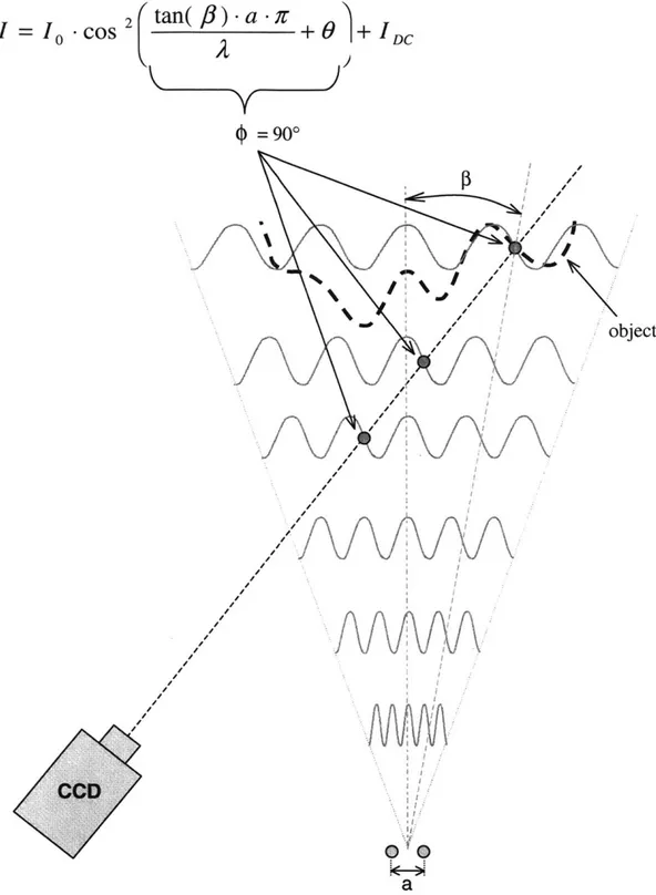
coherent light to "paint the world with interference fringes". As illustrated in Figure 2.1,

two laser beams are focused by a lens into two "source points" at the focal plane. After

the focal plane, the two beams diverge and eventually overlap to form the sinusoidal

-R 4d~ a 2

tan(#i)

ag

in this "fringe space" depends on the distance of the plane from the focal plane and on the

spatial separation of the two source points:

d 2.R

a

Here d is the spacing of the fringes, A is the optical wavelength, R is the distance from the

focal plane to the given interference plane, and a is the separation of the two source

points. The spatial phase of the global fringe pattern can also be varied by changing the

relative phase 9 of the two interfering laser beams. In fact, the intensity at a given point

in the fringe space can be represented by a raised cosine function [12]:

I= 10 .Cos 2 tan(p)-a -r + 0 + Ic

where 6 is defined in the diagram, Io is the amplitude of the fringe pattern, and IDc is the

fixed background illumination level. Note that both Io and IDC will change as the laser

light intensity, background illumination level, and surface reflectivity vary across the

object, and as the path difference between the interfering beams approaches the

coherence length of the laser light. The raised cosine term in the equation, however,

depends only on the location in the fringe space and on the controllable parameters of the

AFI system.

The following sections describe two related ways of extracting depth information

about a given point in the fringe space. Both approaches recover the angular coordinate

#,

#

at a fixed point source separation a. Spectral estimation looks at the local intensity

variation as the point-source separation a is changed.

2.2 Depth extraction through spatial phase estimation

As shown in Figure 2.2, by measuring the wrapped phase of the fringe pattern

imaged by a pixel in a CCD array (900 in this case), one can isolate several discrete locations along the line of sight of the pixel where the imaged region of the object might

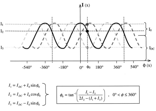
lie. One way of determining the spatial phase at a given pixel is shown in Figure 2.3. As

information theory dictates, by taking three measurements of a sinusoid of known

frequency (determined by the point source separation in this case), one can determine all

three of its unknown parameters - amplitude, offset, and phase (with a 3600 ambiguity). This can be done robustly by shifting the phase of the entire projected fringe pattern, and

measuring the corresponding intensities at each pixel independently. As shown in Figure

2.3, an even sampling and a simple formula results from ±90' phase shifts of the fringe pattern. Since only the spatial phase is of interest for triangulation, the amplitude and

offset parameters are not explicitly calculated.

In order to disambiguate between the possible locations of the imaged point in the

fringe space, we must unwrap the measured phase. One way to achieve this is to project

larger "reference" fringes onto the object. This is shown in Figure 2.4. If a reference

fringe is large enough to cover the entire depth extent of the object, then the phase

measurements with the finer fringes can be completely unwrapped. On the other hand, a

small phase measurement error of a reference fringe that is too large may result in a 360*

I

I0

8)-a

-

Afv/VV~\

NVW

Figure 2.2 Mapping fringes to depth using spatial phase estimation

object I I / I / I / / I I / I / I I / I / /

Ii ---12 13 (x) '0 IDC -540* -360* -1800 00 $o 1800 3600 540* 0 (x) I, = I D o sin

#

Figure 2.3 Estimating spatial phase by phase-shifting the fringes ± 900

I I i I

-5400 -360* -1800 00 1800

I i I

3600 540*

(x)

Figure 2.4 Principle of phase unwrapping using larger reference fringes '

between the density of a set of fringes, and the density of the reference fringes used to

unwrap them. Once the fringes are unwrapped, however, they can be used as a reference

to unwrap an even more dense interference pattern. Since finer fringes result in better

resolution', this process can be iterated until the finest fringes are unwrapped.

2.3

Depth extraction through spectral estimation

The concept of spectral estimation in AFI is illustrated in Figure 2.5. Variation in the separation of the two point-sources causes a stretching of the fringes (as in an

accordion). As required by the raised cosine function, the intensity at any given point in

the fringe space oscillates sinusiodally as a result, where the oscillation frequency is a

function of the angle

#.

(as long as the location of the null fringe is known).

One way to determine the oscillation frequency at a given point is to move the

point-sources apart and count the number of fringes that pass by. This requires hundreds

of image frames for a single surface reconstruction. Another tactic is to use only a few

point source separations, and use a statistical minimization routine to fit a sinusoid to

these samples. This approach, however, can be very computationally-intensive. As a

result of these practical drawbacks, the phase estimation technique was chosen in favor of

I

(

a .r

2.4 Benefits of AFI

Accordion Fringe Interferometry extends the state of the art in 3D measurement.

Some of the benefits that AFI has to offer for a wide range of applications including

high-speed and portable 3D imaging are listed below.

* Resistant to propagation of errors: Because phase is calculated and unwrapped for each pixel independently, errors in range estimation are confined to their

corresponding pixels.

" Well-behaved at sharp edges: Unlike several other 3D techniques which exhibit

discontinuities and other anomalies at sharp edges of the targeted object, AFI is

robust against such discontinuities. Due to the unwrapping process, a

phase-measurement error resulting from a sudden jump within a region imaged by a single

pixel, will be confined to at most 3600. Furthermore, due to the pixel-independent

phase measurement technique, any such errors will not affect neighboring pixels.

e Insensitive to variations in illumination level: Because triangulation depends only on

the phase and frequency of the fringe pattern, variations in amplitude or bias of the

fringe pattern over the extent of the object are inherently compensated for. Although

intensity variations do reduce the dynamic range of the CCD available to some

regions of the object, simulations have shown that the phase estimation technique is

robust even with two or three bits of quantization.

* Parallel acquisition, parallel processing: Because all pixels are acquired

simultaneously by the CCD and range is calculated independently for each pixel, this

technique is fit for parallel processing. Modularity of the steps involved in measuring

* Modest processing and memory requirements: The computation involved in

determining and unwrapping the phase for each pixel and performing a triangulation

calculation is comprised of only a few dozen operations. The memory requirements

are also low - at most three CCD frames need to be held in memory at once (during the phase calculation step). There is a real possibility of real-time video-rate AFI

processing with dedicated hardware.

" Simple hardware: An AFI system consists of a CCD detector, a fringe projector, and

the associated software and electronics. Most of these components are off-the-shelf

items and are relatively economical.

2.5

Current state of AFI

The Accordion Fringe Interferometry technique has evolved through many

iterations of method and prototype. The current AFI system is not only a successful

laboratory prototype, but is being tested at a major airplane production facility to measure

aircraft body panels as part of the quality control process.

One would also like to expand AFI into areas where the requirements are

altogether different from industrial metrology, where more important than high resolution

are low cost, speed, portability, and automation. Clearly, many 3D applications would

benefit from the simplicity and robustness of the AFI method.

A recent invention which provides a solid-state method of projecting and

electronically controlling interference fringes using an Acousto-Optic Modulator may be

instrumental in overcoming the difficulties of bringing AFI into the world of high-speed

Chapter 3

Implementation of AFI projector using acousto-optics

Accordion Fringe Interferometry requires precise control over the phase and

frequency of a projected interference fringe pattern. The AFI projector currently used for

industrial metrology relies on translation of optical components, and its precision and

speed is limited by the motion-control system. This chapter presents an alternative

solid-state design of an interference fringe projector using an Acousto-Optic Modulator that is

geared towards applications that require a portable high-speed 3D imaging system.

3.1 Physics of an Acousto-Optic Modulator

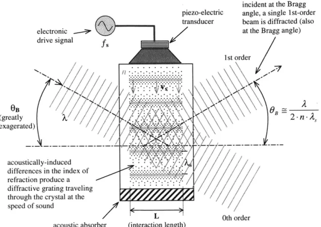
An Acousto-Optic Modulator (AOM), consists of a crystal in contact with a

piezo-electric transducer (PZT), as depicted in Figure 3.1. By driving the PZT with a

sinusoidal electric signal (typically around 100 MHz), a traveling sound wave is

piezo-electric transducer electronic .- &

drive signal _f,

acoustically-induced differences in the index of refraction produce a diffractive grating traveling through the crystal at the speed of sound

Only when the light is incident at the Bragg angle, a single 1st-order beam is diffracted (also at the Bragg angle)

S 2 _2-n

A

acoustic absorber (interaction length)

opposite end of the crystal. When coherent light is made to pass through this excited

medium, several phenomena are observed:

Bragg Diffraction

A laser beam incident on the traveling sound wave is diffracted in a phenomenon

known as Brillouin scattering[13]. The combined effect of acousto-optic interaction in a

material that is comprised of different scattering regions can be understood as follows.

The acoustic wave consists of sinusoidal perturbation in the density, and hence

the refractive index of the material. At a given moment in time, for a sufficiently long

acousto-optic interaction length L, this wavefront of index of refraction gradients can be

thought of as an array of partially-reflecting "mirrors" [14]. The incident beam will be

diffracted by a given mirror in this array only if all the scattering regions along the length

of the mirror contribute in phase. This can happen only if the angle of incidence at each

mirror is equal to the angle of diffraction (as would be expected for a mirror).

Furthermore, the beam will be diffracted in a certain direction only if each mirror in the

array contributes in phase with the other mirrors to the overall diffracted wavefront.

These constructive interference conditions are combined in what is known as the Bragg

diffraction condition:

2A4 sin6B

no

where ks is the acoustic wavelength within the medium, X is the wavelength of light in

free space, no is the index of refraction, and O6= = OB is the Bragg angle (typically a few degrees). Note that due to the necessary equality between 0; and OB, only the first-order

beam is diffracted under this condition, and is angularly separated from the zeroth-order

beam by 2 0 B.

Based on the mirror model, one may wonder why OB can not be a multiple m of

X/no. While the Bragg angle is not unique for diffraction from discrete surfaces, it can be

shown that due to the continuous nature of the index of refraction gradients in the crystal,

m=1 is the only mode that will result in acousto-optic diffraction [14].

When the acoustic wavefront is very thin, the acousto-optic interaction length L is

short and the acoustic wavefront is better modeled by an array of point scatterers rather

than by an array of mirrors. Thus the phase matching condition that was used to pin the

angle of diffraction to be equal to the angle of incidence for a mirror does not hold in this

case, and multiple diffraction orders exist as in the familiar case of a diffractive grating.

This situation is known as the Raman-Nath regime of acousto-optic interaction [15].

The transition between the Raman-Nath regime and the Bragg regime is not clear cut, but

by convention is defined using the parameter

Q

Q = A

For Q < 0.1, the operation is said to be Raman-Nath. For

Q

Bragg regime of acousto-optic interaction, where the interaction length is long, and only

Amplitude Modulation

The amplitude of the acoustic signal determines the gradients in the index of

refraction in the crystal, and thus the reflection coefficients of the analogous array of

mirrors. As a result, the optical energy transferred from the zeroth-order beam to the

first-order beam can be rapidly and precisely controlled by amplitude-modulating the

drive signal to the PZT. Typically, diffraction efficiency of -90% and modulation

bandwidth of ~1MHz can be achieved. Since the two beams can be easily separated, this

effect is commonly used to modulate the intensity of a laser beam, and leads to the name

of AOM.

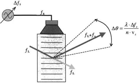
Deflection

Another use of the AOM stems from the fact that even if the angle of incidence

and the acoustic frequency do not satisfy the Bragg condition exactly, diffraction still

occurs. If 0; and ks do not stray too far from the Bragg condition, destructive interference

only slightly dims the first-order beam. As illustrated in Figure 3.2A, however, the angle

of the beam, is no longer restricted to the Bragg angle 6B, but will deflect slightly as a function of acoustic frequency, pointing in the direction where the destructive

interference is least. In fact, for small AO and OB, AO is related to Afs in an approximately

linear fashion [14]:

AO -Af. AB= A.A

where vs is the velocity of sound in the medium. Typically, AO ~ 0.50B can be achieved

on either side of OB before the amplitude of the diffracted beam falls by 3dB compared to

the amplitude at 0_B.

Diffraction of multiple beams

Although the operation of an AOM is best understood by studying the effects of a

single sinusoidal acoustic wavefront, a superposition of several frequencies in the drive

signal will result in the superposition of several acoustic wavefronts, and will generate

several angularly-separated first-order beams. This effect is shown in Figure 3.2B. Since

the amplitude and frequency of the drive signal can be independently controlled, so can

the amplitude and direction of each of the multiple first-order beams!

Optical phase and frequency shifts

So far we have focused on the acoustic wavefront as seen by the incident laser

beam at a given moment in time. Since sound propagates much slower than light, this is

a good approximation for understanding the effects of acousto-optic interaction on the

direction and amplitude of the diffracted beams. However, conservation of momentum

requires that the traveling acoustic wavefront must also impose a unique Doppler shift

fs;

= vs/ksi on each of the diffracted first-order beams relative to the unperturbed zeroth-order

beam. In addition, the acoustic wave adds a phase shift to the diffracted optical beam, so

that a relative phase shift between two superimposed acoustic waves results in the same

n-v

AL

A. Direction of the 1st-order beam can be controlled by varying the acoustic frequenicy

compound RF drive signal with individually controlled frequencies and amplitudes

B. Multiple acoustic frequencies deflect multiple 1st-order beams

Figure 3.2 Beam deflection using an acousto-optic cell

Afs

7/

fL

fsi

have major repercussions for generating and controlling an interference pattern using an

AOM.

3.2 Generating stationary interference fringe patterns

3.2.1 Projecting accordion fringes

As discussed in the previous section, an AOM can be used to separate a laser

beam into two or more beams, and to electronically control the angular separation,

amplitude, and phase of the beams. The AFI technique, however, relies on the ability to

combine and interfere coherent beams near the object of interest. The simplest way to

achieve this using acousto-optics is to place a lens in the path of the angularly separated

beams produced by the AOM. The function of a lens is to convert angular separation

between incident planar wavefronts into spatial separation at its focal plane. The

separation between the corresponding focal points, or "source-points", is an

approximately linear function of the angular separation of the diffracted beams, and

remains the same no matter where the lens is placed in the optical path of the beams. If

we choose a lens with a small enough focal length to cause the beams to overlap in the

region of interest, a fringe pattern will result with the fringe spacing simply related to the

source-point separation, to the angular separation, and thus to the frequency difference

between the two beams.

One such arrangement is depicted in Figure 3.3. Here a superposition of two

frequencies is used to drive the AOM. The compound drive signal is generated by

lens fL + + f "source points"

fm

/

fixed center frequency

fc.

separation allowed by the bandwidth of the AOM, thereby producing accordion motion

of the interference fringes.

It is also possible to generate an interference pattern using a single drive

frequency by interfering the first-order beam with the zeroth-order beam. This has the

advantage that a substantially (-2.5x) larger source-point separation is possible, resulting

in finer fringes and better resolution. However, there are several difficulties with this

approach:

* The point of symmetry of source-point motion is not fixed as it is in the compound

drive case, and the null of the fringe pattern will shift as the source-points are drawn

apart. This effect can be easily compensated for in the AFI mathematics.

* The lowest drive frequency allowable by the bandwidth of the AOM limits the

proximity of the source points. As a result it is not possible to generate large

reference fringes, calling for other phase unwrapping strategies in the AFI method.

As a consequence, the compound drive approach is currently the preferred strategy.

3.2.2 Freezing the fringes

Although the apparatus described so far causes two diffracted beams to interfere,

fringes do not appear across the interference plane. The problem lies in the fact that the

interfering beams have a relative Doppler shift. As a result, the light intensity at any

given point on an interference plane will oscillate in time at the difference frequency as

very small compared to the optical wavelength, at any moment in time constructive and

destructive interference between the two beams still occurs across the interference plane

and results in the familiar full-contrast fringe pattern. These two observations require

that the interference fringe pattern travel rapidly across the interference plane, as the

acoustic wave travels across the AOM. Any exposure time that is longer than the period

of the traveling interference pattern (i.e. 25ns for a difference frequency of 40MHz), will

show a featureless blur.

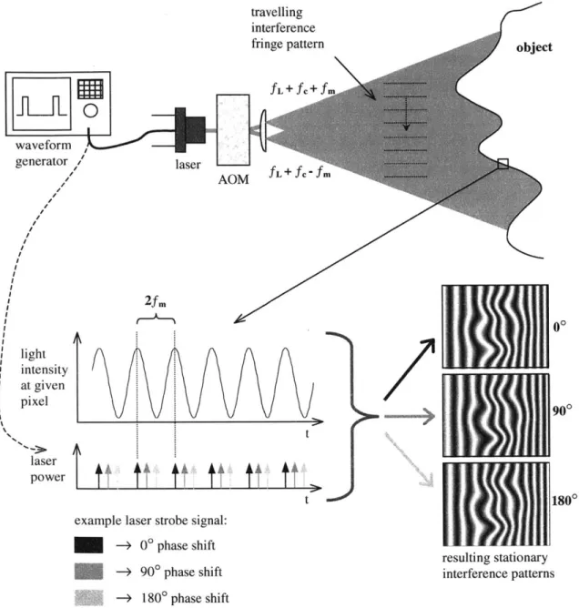
The key concept that makes the AOM technology useful for AFI is that the

traveling interference fringes can be "frozen" in time at any spatial phase desired by

amplitude-modulating the radiation intensity in sync with the AOM drive signal. This is

illustrated in Figure 3.4. As the intensity at a given point on the illuminated object

oscillates at the difference frequency of the two interfering beams, 2fm in the case of the

compound drive fringe projector, strobing the laser power at exactly the same frequency

will "freeze" the interference pattern in time at a particular point in the oscillation2. The

synchronization between the laser and the AOM control signals can be easily

accomplished by digitally synthesizing the signals using the same reference clock, for

example. The relative phase between the two interfering beams, and hence the spatial

phase of the resulting fringes, can be precisely controlled either by changing the phase of

the compound signal driving the AOM, or by changing the phase of the laser strobe

signal. The figure shows simulated stationary interference fringe patterns that would be

projected onto an object with 00, 90', and 1800 relative phase shifts between the laser and

the AOM signals.

travelling interference fringe pattern fL + fc + fn AOM fL +fc fm

'Lii

It

ft ft ft ft

--> 0 phase shift

E

Figure 3.4 Freezing and phase shifting a traveling interference pattern

object 2f m light intensity at given pixel laser power

One clear disadvantage of strobing the laser is the inherent loss of light power.

This is a serious issue, since the projector's light output capability limits the distance of

the objects to be imaged (to a few meters in a practical case), and is a major factor in the

overall cost of the system. It turns out, however, that it is not necessary to strobe the

laser with short pulses to obtain a stationary interference pattern. In fact, any light

intensity modulation will result in the appearance of a stationary sinusoidal fringe pattern

with some contrast measure between 0% (in the case of no modulation) and 100% (in the

case of modulation with a train of impulses). The choice of the modulation waveform

becomes a tradeoff between the desired contrast of the stationary fringes and the power

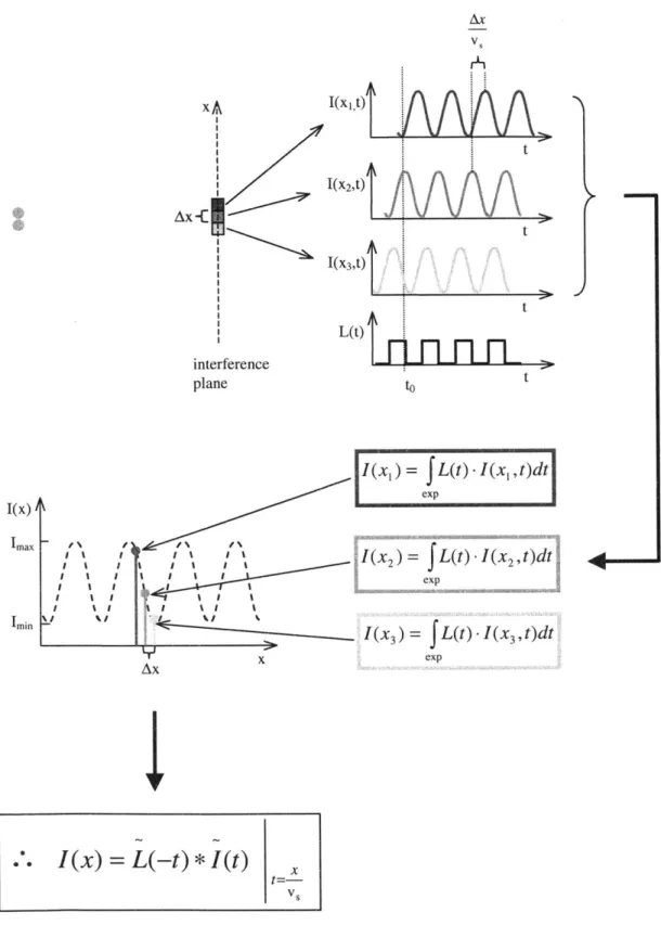
output desired from the laser. This can be understood by examining Figure 3.5.

Without any light intensity modulation, due to the traveling interference fringes,

each pixel i of three adjacent pixels on the interference plane would see intensity

oscillations I(xi,t) at the difference frequency that are out of phase with each other by a

time interval t = Ax/vs, where Ax is the separation of the pixels. The actual intensity at each point, I(xi), accumulated over the exposure time, is obtained by multiplying I(xi,t) by

the laser amplitude L(t) at each instant in time, and integrating over the exposure time.

The reader may recognize this repetitive phase-shift/multiply operation used to obtain the

interference intensity in space as a periodic convolution of a time-dependent intensity

oscillation I(t) with the reversed laser drive signal L(-t), evaluated at t = x/vs.

The same result can be derived mathematically by noting that the traveling fringes

can be described as a function of time and space:

x

t--Ax VS I(xit) t2Xt I*xt xA interference plane t t L(t) to t I(xI) L (t -I(xat)dt ,I~, I =fL t Ia (x, 'a I ... ... Y Ax

x

t)dt

1(x)=

L(-t)* 1(t)

Figure 3.5 Using periodic convolution to model fringe intensity

I(x3,t) I(x)4t Imax I.mm ,' j I' I I ~ I I 'a I I 'a I I 'a I I 'al ~, 'aa/

4---,

As discussed above, intensity in space can be obtained by multiplying I(x,t) by L(t), and

integrating over time:

I(x)=f L(t)-

f

exp v}

For an exposure time that is much longer than the least common multiple of the periods

of the two waveforms, this is equivalent to periodic convolution:

I(x) = L(-t) * I(t) _t=--,

V,

From the above discussion it is evident that independent of the light intensity

modulation, the fringe pattern I(x) must be a superposition of identical raised sinusoids

that are phase-shifted in space relative to each other, and thus must be itself be a raised

sinusoid with the spatial frequency determined by the source-point separation. To

simulate the effect of various laser drive waveforms on the contrast of these stationary

fringes, we can approximate I(x) by discretizing L(t) and I(t) and performing circular

convolution on an integer number of cycles of the two waveforms. Since circular convolution corresponds to multiplication in the Discrete Fourier Transform domain, it

can be approximated in Matlab (or any other signal processing tool) by taking the inverse

FFT of the product of FFT's of the two signals. The following table compares the

contrast and average intensity I (normalized by the CW laser output power I,.,) of the

fringe patterns produced by several different laser drive waveforms, where we define as a

Laser drive waveform M I/Ic

(periodic with difference frequency)

10% duty-cycle square wave 0.98 .11

50% duty-cycle square wave 0.63 .50

sinusoid 0.50 .50

When choosing the waveform to drive the laser, one must consider the amount of

available light that reaches the object, the reflection properties of the illuminated object,

as well as the sensitivity and dynamic range of the detector. If the laser is much more

powerful than necessary, strobing the laser with short pulses will produce nearly perfect

contrast and still provide sufficient light to reach the saturation limit of the detector. If

the light power comes at a cost, then the tradeoff between contrast and light intensity

becomes a more difficult engineering decision. It's important to note that this tradeoff is

highly nonlinear. Halving the duty cycle from 10% to 5%, for example, will throw away

half of the laser power, but will hardly change the already excellent contrast.

Furthermore, as illustrated by the sinusoid results, some waveforms are preferable to

others with respect to both contrast and light power. In fact, among waveforms that

produce the same average light output, the square wave offers the best performance since

it is the most compact in the time domain, resulting in the least variation in the phases of

the superimposed sinusoids that make up the stationary fringe pattern.

The above analysis applies to CW (or continuous-wave) lasers. A variety of

pulsed lasers exist, which concentrate all of their energy into periodic pulses that are

much shorter than the period of the traveling interference pattern (e.g. <<25ns). If such a

laser can be pulsed at the difference frequency of the interfering beams, fringes with

3.3 An implementation of an acousto-optic projector

In the previous section we have seen how to generate a stationary interference fringe pattern and precisely and rapidly control it's spatial phase, spatial

frequency,

and intensity without a single moving elemen? using an electronic signal.

This chapter addresses some of the issues associated with implementing a

prototype of such a high-speed solid-state acousto-optic projector.

3.3.1 Target Application

Design decisions for an AFI projector depend on tradeoffs between the range and

extent of objects to be imaged, the desired resolution, and the imaging rate required.

Since our primary objective is to demonstrate the concept of a high-speed AFI projector

and to show that it can be applied to high-speed 3D imaging, a target application that

would benefit from high acquisition speed but does not require high resolution or a large

area of coverage is desirable.

One such application is 3D imaging of lip motion during speech. A 3D video of

moving lips would be useful for generating models for speech analysis, lip reading, and

voice recognition applications. Lips would also be a good target for the first prototype of

the AOM AFI projector for the following reasons:

e The resolution requirements are minimal for modeling the shape of lips. Since lips

have a smooth curved surface, resolution on the order of 1mm would be sufficient to

sample the overall shape. Resolution is in part a function of the density of fringes

projected on the object (and hence the maximum source-point separation achievable

with the AOM), and in part a function of the resolution and dynamic range of the

CCD detector. A few dozen fringes across the lips should be more than sufficient.

As will be seen shortly, this can be achieved with a variety of AOMs and can be

well resolved with many high-speed CCD cameras.

" The extent of the lips is limited and they can be imaged at close range. As a result,

projector power output of only a few milliwatts should be sufficient to illuminate the

lips a few feet away, even for very short exposure times and low sensitivity

characteristic of high frame-rate CCD cameras. Such power levels are available in a number of inexpensive diode lasers, and are considered eye-safe even a few inches

away from the projector.

" The shape of the lips is smooth, simplifying the phase unwrapping steps in the AFI

process.

" Lips are not prone to specular reflection and can be easily coated with white powder

to improve their reflectivity properties.

3.3.2 System design

Figure 3.6 shows a block diagram of a prototype acousto-optic AFI projector that

was built and tested in the laboratory. A photograph of the actual setup is shown in

Figure 3.7. The following subsections address design considerations for each system

Optics LENS IRIS Electronics r--- ---~---~-~---~~~~~~~~~~~~|---I AWG HIGHPASS FILTERAMPLIFIER MIXER L XTAL

9

Source of coherent radiation

Choosing an illumination source involves weighing of several parameters: power,

wavelength, modulation bandwidth, coherence length, and of course cost. Since the

object proximity is on the scale of a few feet for this prototype, it turns out that a 20mW

laser would be sufficient to illuminate most objects. The common diode laser seems like

a natural choice for providing this kind of power output. Not only are diodes of this

power range commonly available, but they are much less expensive than other CW laser

technologies of comparable output power. In addition, unlike most other lasers, many

diode lasers can be modulated at rates in excess of 50 MHz -- sufficiently rapidly to be able to generate a high-contrast stationary interference pattern -- without the need for an external amplitude modulator. Some pulsed diode lasers are even available.

On the other hand, diode lasers typically cover longer wavelengths from red to

infrared. One would expect that a green or blue laser would produce finer fringes,

resulting in better resolution. In fact, this is not the case due to the physics of the AOM.

As the reader may recall, the angular separation between the diffracted beams, and hence

the point-source separation, is directly proportional to the optical wavelength. The spatial

frequency of interference fringes, on the other hand, is directly proportional to

point-source separation, and inversely proportional to the optical wavelength. As a result, there

is no net dependence of the fringe spacing on the optical wavelength! This can be understood intuitively from conservation of momentum. Since photons with longer

wavelengths have less momentum than photons with shorter wavelength (momentum=

h*27/0), they are deflected by a proportionately larger angle by the oncoming sound

response. Not by accident, most CCD spectral response curves happen to coincide well

with the commonly available red and infrared diode lasers.

One disadvantage of laser diodes compared to HeNe lasers, for example, is a very

short coherence length: a few millimeters or less. Although this may not be enough in a

projector with several widely-separated optical paths, in the AOM projector both beams

share the same optical path and the coherence length required for high-contrast fringes is

simply the greatest accumulated path difference at the interference plane -- i.e. the number of fringes in the interference pattern multiplied by the optical wavelength. For

this prototype, for example, the required coherence length is only -20gm. This is almost

achievable with some LED's!

The laser chosen for this system is a Power Technology PMT series module with

a 685nm 40mW diode laser. This very economical laser module is equipped with a TTL

trigger input, making it trivial to interface and synchronize with the RF electronics that

generate the AOM drive signal, and can be modulated at over 100MHz. While this is

sufficient to obtain stationary fringes over the entire AOM bandwidth, the -5ns step

response does not allow duty cycles below -30% with a difference frequency of 40 MHz,

for example, thereby somewhat limiting the contrast at the largest point-source

separations. A laser with an even faster modulation capability would be desirable to

obtain high-contrast interference with higher bandwidth AOM's and even greater fringe

Detector

Since the speed of the system is limited by the frame rate of the detector used,

choosing a high-speed CCD camera is essential. However, as the exposure time is reduced, a stronger laser source is required to sufficiently illuminate the object. In

addition, due to the short readout time, pixel count, bit depth, well depth, and

signal-to-noise ratio of the CCD are in general sacrificed.

In this case the 8-bit 256x256 Dalsa MotionVision CA-D7 area scan CCD camera

was used with a Nikon 60mm 1:2.8D AF Micro Nikkor lens. Although this camera is

capable of rates of up to 955 frames per second, it was used at only a fraction of this

speed (90 fps) due to the available software and the capture speed of the frame grabber at

hand. As simulations have shown, the AFI technique is fairly insensitive to quantization

noise, and even four-bit signal quantization is more than enough to achieve the desired

resolution for the target application. Also, because of the low resolution requirements, a

256x256 CCD array provides a good sampling of the fringe pattern. Furthermore, even with the lens partially stopped to increase the depth of focus, a few milliwatts of output

from the projector is enough to saturate the 11-ms exposures of the CCD because of the

proximity of the target in this case. Nevertheless, CCD speed-vs.-performance tradeoffs

AOM

There are many kinds of AOM's available, geared towards different applications,

different wavelengths, as well as different performance requirements. Listed below are

some important characteristics to look for when choosing an AOM for an interference

fringe projector.

* Interaction Material is the crystal material carrying the acoustic wave. Commonly

used materials are dense flint glass, PbMoO4, TeO2, germanium, and quartz. Each

material has unique optical and acoustic properties. TeO2, for example, has the

slowest acoustic velocity (0.617mm/is) [14] and hence is used to achieve large

deflection angles and high modulation rates. Quartz, on the other hand, transmits

well in the UV range, while germanium is used mainly for far-infrared applications.

PbMoO4, which is the most commonly used material, has a relatively slow acoustic

velocity (3.63mm/gs) and is insensitive to laser polarization. Most of the AOM

models are available in several broad antireflection coating ranges.

" Center Frequency corresponds to the frequency of the drive signal that would meet

the Bragg condition when the input to the AOM is aligned at the Bragg angle.

f 2n -sin 6_B -Vs

As the Bragg condition dictates, the higher the center frequency the larger the Bragg

angle for a given interaction material and a given optical wavelength, and hence the

larger the separation between the first-order and the zeroth-order beams. Thus, a

large center frequency would be desirable for a single-frequency drive AOM

projector discussed earlier. Note that as the typical center frequencies range from

40MHz to 300MHz, it becomes increasingly challenging to synthesize and power the

AOM drive signal.

* RF bandwidth refers to the range of drive frequencies corresponding to the range of diffraction angles (a.k.a. scan angle) over which the first-order beam remains within

3dB of its intensity at the Bragg angle. This bandwidth, and the corresponding scan

angle, varies as a function of the optical wavelength, center frequency, and the

acousto-optic interaction length [17]:

n - v2 _v

Af = 1.8 - S =1.8.

2v -f.L 2 -sin(GB).L

Note that the RF bandwidth is wavelength-independent, and that it falls as the center

frequency increases, unless of course the interaction length L is adjusted to

compensate. In the case of the compound drive AOM projector, the largest possible

Af is preferable (regardless of the center frequency) since it results in the largest

separation between the first-order beams, and hence the finest fringes. One must also

take into account the modulation bandwidth of the laser, since for the largest

point-source separation it will have to be amplitude-modulated near Af to achieve a

reasonable contrast in the fringe pattern.

* Diffraction Efficiency is the ratio of the intensity in the diffracted beam(s) to the

intensity of the original beam, and is a function of the properties of the material, of

the interaction length, and of the strength of the acoustic signal [14]:

I'f'acted _{= sin14}

0.6328 _{. L* MI}

where Mw is a material-dependent figure of merit. Evidently, diffraction efficiency

can be increased by supplying more power to the AOM, and values above 50% can

by typically reached. While the highest possible diffraction efficiency is desired for

the compound-drive projector, a 50% diffraction efficiency would be ideal for the

single frequency drive projector that uses the first and zeroth-order beams to generate

a fringe pattern.

* Active aperture is the maximum diameter of the laser beam that will fully interact

with the traveling acoustic wave. An elliptical aperture is preferable for use with a

diode laser, since the output of most diode lasers has an elliptical crossection.

* Resolution is characterized by the number of resolvable beams (a.k.a. "spots",)5_{, also}

known as the rAf product, where t is the time required for the sound to cross the

diameter of the optical beam. As expected, resolution is inversely related to the

well-known divergence ratio, X/D. Thus, AOMs with larger active apertures produce more

resolvable spots and tend to be used as deflectors. Note that AOM resolution is

irrelevantfor the AFI projector. Because the laser beams have a Gaussian intensity distribution, they expand in a hyperbolic fashion as they propagate [14], and thus do

not have to be resolved in the Rayleigh sense to generate an interference pattern. This

is illustrated in Figure 3.8. In fact, it is possible to generate almost arbitrarily large

fringes using the AOM technique simply by driving the AOM with a compound

signal with a very small difference frequency.

* Rise time is the time for the diffracted laser beam intensity to rise from 10% to 90%

of its maximum value in response to a step in the amplitude of the acoustic wave, and

lens "source points" -- apparent origins of light

- are well defined even if the Gaussian

beams are not resolved from each other

determines the modulation bandwidth of the AOM. Since the entire aperture must be

filled with the new acoustic level before the diffracted beam fully responds, the rise

time is proportional to the ratio of the aperture size and the acoustic velocity. Thus,

while AOMs with a large active aperture are good beam deflectors, they are slow

beam intensity modulators. Rapid beam intensity modulation is not generally

important for an interference pattern projector. However, since rise-time is closely

related to the frequency and phase modulation bandwidth, it may be an important

consideration for interference pattern projection applications where high-bandwidth

active drift compensation is important.

* Power requirements for achieving optimum diffraction efficiency depend on the

material used, the optical wavelength, as well as on the acousto-optic interaction

length, as the diffraction efficiency equation indicates. One or two Watts of drive

power are typically sufficient for red and infra-red wavelengths. Significantly

overdriving the AOM would actually result in loss of diffraction efficiency and

eventually possible damage to piezo-electric transducer and internal power-matching

electronics.

With the above considerations as well as cost and size in mind, Isomet's 1205-C2-804

AOM coated for the operational wavelength of 685nm was used for this prototype. This

device is only 22 x 16 x 51 mm3 _{in size, has a center frequency of 80MHz, and has an RF} bandwidth of 40MHz, corresponding to a maximum angular separation of -0.6' between