HAL Id: hal-00270764
https://hal.archives-ouvertes.fr/hal-00270764
Submitted on 7 Apr 2008HAL is a multi-disciplinary open access
archive for the deposit and dissemination of sci-entific research documents, whether they are pub-lished or not. The documents may come from teaching and research institutions in France or abroad, or from public or private research centers.
L’archive ouverte pluridisciplinaire HAL, est destinée au dépôt et à la diffusion de documents scientifiques de niveau recherche, publiés ou non, émanant des établissements d’enseignement et de recherche français ou étrangers, des laboratoires publics ou privés.
A parallel in time approach for quantum control: the
parareal algorithm
Yvon Maday, Gabriel Turinici
To cite this version:
Yvon Maday, Gabriel Turinici. A parallel in time approach for quantum control: the parareal algo-rithm. IEEE Conference on Decision and Control, Dec 2002, Las Vegas, United States. pp.62-66. �hal-00270764�
A parallel in time approach for quantum control:
the parareal algorithm
Yvon Maday
Laboratoire Jacques-Louis Lions
Universit´e Pierre et Marie Curie
Boˆıte courrier 187, 75252 Paris Cedex 05 France
[email protected]
Gabriel TURINICI
INRIA Rocquencourt, Domaine de Voluceau
Rocquencourt - B.P. 105, 78153
Le Chesnay Cedex - France
and
CERMICS-ENPC, Marne la Vall´ee, France
[email protected]
Abstract
The numerical studies of control problems in quantum chemistry go through the computer simulation of the dynamical phenomena in-volved. These simulations are in many cases too expensive to be carried out for complex systems, precluding thus treatment of interest-ing practical situations.
In a context of fast increasing in both the CPU power available on typical workstations and of the number of computers that can be con-nected through high speed networks, the diffi-culty lies rather in how to obtain “real time” solutions than in the amount of CPU power available (which becomes to exceed the needs). In this context, the ”parareal” time algorithm that parallelize in the time direction the ef-fort required to solve evolution equations has been introduced in previous works [4, 3, 2]. The theoretical modifications required in
or-der to apply this algorithm to quantum control problems together with numerical evidence is the main topic of this paper.
1 Introduction
The control of quantum mechanical systems has long tradition in using numerical computer simulations in order to model and understand intricate practical situations encountered in complex laboratory experiments [1]. However, even when these simulations refer to simple systems they are very costly in computational resources and require long times to be carried on. On the other hand, in the nowadays hard-ware environments, CPU power is not such a scarce resource and, for instance, the price of constructing a high-speed networked cluster of PCs is now within the financial means of most academic departments. The bottleneck comes thus not from the lack of processors but rather from the intrinsic sequential nature of
the simulations used in quantum control which mostly deal with evolution equations. In or-der to address this situation, a discretization scheme parallel in time was proposed [4]; this scheme, called the “parareal” time scheme, de-composes the time evolution in several inde-pendent sub-problems which are evolved simul-taneously (in parallel) on different processors. Necessary corrections are then applied to the results thus obtained in an iterative manner leading to (fast) convergence to the exact result (allowing to envision real time simulations). This scheme was applied with success to the linear [4] and non-linear PDEs [3], to the equa-tions of the molecular dynamics [2] and also for a first application to control problems [5]. Within this context, the goal of this paper is to discuss the specificities required by the appli-cation of this “parareal” time scheme to quan-tum control settings. The necessary dynam-ical equations are presented in Section 2 to-gether with the adequated algorithms to solve the control problem. The parareal scheme is presented in Section 3 followed in Section 4 by implementation details and numerical results. Finally, a discussion and some perspectives are developped in Section 5.
2 Dynamical Equations
Consider a quantum system with internal
Hamiltonian H0 without control interaction
that is prepared in the initial state ψ0(x) (with
kψ0kL2(Rγ) = 1) where x denotes the
rele-vant coordinate variables; the state ψ(x, t) of the system satisfies at each time t the time-dependent Schr¨odinger equation
(
i¯h∂
∂tψ(x, t) = H0ψ(x, t)
ψ(x, t = 0) = ψ0(x), (1)
In the presence of an external interaction taken here as an electric field modeled by a coupling operator given by an amplitude ²(t) ∈ R and a time independent dipole moment operator µ
the Hamiltonian H0 is replaced by H = H0−
²(t)µ that gives rise to the dynamical equations to be controlled:
(
i¯h∂
∂tψ(x, t) = (H0− ²(t)µ)ψ(x, t)
ψ(x, t = 0) = ψ0(x) (2)
The optimal control approach is to assess the fitness of the final state ψ(T ) = ψ(x, T ) through the introduction of a cost functional J to be optimized; this cost functional includes on one hand terms that describe how well the objective has been met and on the other hand terms that penalize undesired effects. One sim-ple examsim-ple of cost functional is
J(²) =< ψ(T )|O|ψ(T ) > −α
Z T
0 ²
2(t)dt (3)
where α > 0 is a parameter and O is the ob-servable operator that encodes the goal. In mathematical terms, the observable O is a self-adjoint operator that acts on ψ(T ); larger the value < ψ(T )|O|ψ(T ) > better the control objectives have been met; note that in gen-eral attaining the maximal possible value of < ψ(T )|O|ψ(T ) > requires a large laser
flu-ence RT
0 ²2(t)dt; the optimum evolution will
therefore strike a balance between using a not too expensive laser fluence while simultane-ously ensuring the desired observable has a suf-ficiently large value.
The maximization of the cost functional J(²) can be realized by writing down the Euler-Lagrange critical point equations; a standard way to derive these equations is to introduce an adjoint state χ(t, x) (used as a Lagrange multiplier). The following equations are thus obtained [9]: ( i¯h∂ ∂tψ(x, t) = (H0− ²(t)µ)ψ(x, t) ψ(x, t = 0) = ψ0(x) (4) ( i¯h∂ ∂tχ(x, t) = (H0− ²(t)µ)χ(x, t) χ(x, t = T ) = Oψ(x, T ) (5) α²(t) = −Im < χ(t)|µ|ψ(t) > (6)
One efficient choice for solving in practice the critical point equations (4)-(6) is the
monotonically convergent iterative algorithm of Zhu&Rabitz [9] that can be described by the resolution of the following equations at step k:
( i¯h∂t∂ψk(x, t) = (H 0+ Im<χ k−1|µ|ψk>(t) α µ)ψ k(x, t) ψk(x, t = 0) = ψ 0(x) (7) ( i¯h∂ ∂tχ k(x, t) = (H 0+ Im<χ k|µ|ψk>(t) α µ)χ k(x, t) χk(x, t = T ) = Oψk(x, T ) (8)
Let us also mention the formulation of [6] that was also used here
( i¯h∂t∂ψk(x, t) = (H 0− ²k(t)µ)ψk(x, t) ψk(x, t = 0) = ψ 0(x) (9) ²k = (1 − δ)˜²k−1− δ αImhχ k−1|µ|ψki (10) ( i¯h∂ ∂tχ k(x, t) = (H 0− ˜²k(t)µ)χk(x, t) χk(x, t = T ) = Oψk(x, T ) (11) ˜²k = (1 − η)²k− η αImhχ k |µ|ψki (12)
3 Parareal time discretization Consider a general evolution equation
d
dtu(t) = Au(t) (13)
and define the associated propagator F (t0, t1)
by the requirement that for any u, F (t0, t1)u is
the solution at time t1 of Eqn. (13) for the
ini-tial data u at time t0. Given a final time T and
an initial data u0, solving Eqn. (13) reduces to
computing U (t) = F (0, t)u, 0 ≤ t ≤ T . Let
us introduce intermediary times Tn= n · T /N ,
n = 0, .., N and intermediate time state
snap-shots un, n = 1, ..., N . It is obvious that un are
exactly the values U (Tn) if and only if for any
n = 1, ..., N : un= F (Tn−1, Tn)un−1.
The parareal time scheme proposes to give an iterative method to obtain the sequence
U (Tn), n = 1, ..., N using a coarse
propaga-torG(Tn−1, Tn) that approximates F (Tn−1, Tn)
(n = 1, ..., N ) obtained e.g. by solving a cheap, approximate, yet close to original evolution
equation
d
dtu(t) = ˜Au(t) (14)
The iterative update procedure is then
uk+10 = u0 uk+1n+1 = G(Tn, Tn+1)uk+1n + F (Tn, Tn+1)ukn− G(Tn, Tn+1)ukn (15)
In this scheme, for each iteration k the
compu-tation of F (Tn, Tn+1)ukn− G(Tn, Tn+1)ukn (n =
1, ..., N ) is to be done in parallel and the only sequential part remains the computation of
G(Tn, Tn+1)uk+1n which is cheap since it involves
the coarse propagator.
When this scheme is applied to the setting of the quantum control, a desirable property is that the update formula of Eqn. (15) be consistent with the norm preservation proper-ties of the evolution equation (4): kψ(x, t)k =
kψ0(x)k = 1, ∀t. In order to address this issue
an alternative update scheme will also be used in this work:
uk+10 = u0, uk+1n+1 = RnF (Tn, Tn+1)ukn (16)
where Rn is the rotation in the plane spanned
by G(Tn, Tn+1)ukn and G(Tn, Tn+1)uk+1n
that transforms G(Tn, Tn+1)ukn into
G(Tn, Tn+1)uk+1n . This update formula
will preserve the norm of the state as soon
as the fine evolution F (Tn, Tn+1) is norm
preserving.
4 Choice of coarse propagator and numerical results
In order to test the parareal algorithm for quantum control problems we have chosen the case of a Morse potential type O − H bond. The model was taken to be the one described
in [8] page 1958 (first test case: from ψ0 = |0i
to ψT = |1i, T = 30000 a.u.). The fine
propa-gator F was taken to correspond to the split-operator propagation method (of second or-der in the state and first-oror-der in the field)
with a time step dt = 1 a.u. and a spacial discretization of dx = 0.234 a.u. The coarse propagator G was taken to correspond to the same numerical scheme but with a larger time step, DT = T /N = 10 a.u.; it is therefore DT /dt = 10 times faster to apply the coarse propagator G than it is to compute the fine propagator F .
Remark. One can also think of a coarse
prop-agator that corresponds to the evolution of the system within the space spanned by the first `
eigenfunctions of the internal Hamiltonian H0
(e.g. ` = 10). The numerical results corre-sponding to this approach, not reported here, show promising perspectives but work is still needed in this direction to improve its perfor-mance.
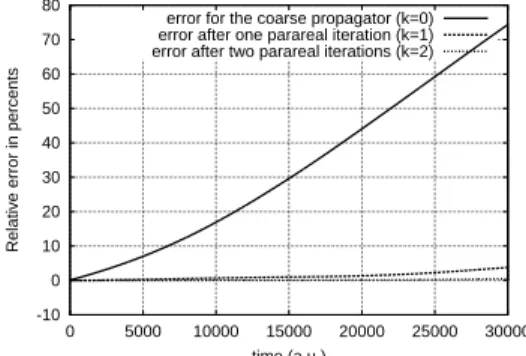
In the first test of our parallel scheme we con-sider that the optimal field ²(t) that maximizes J(²) is known and we check that the parareal scheme is able to recover the evolution of the system. The numerical results are presented in Fig. 1 and 2 where it is demonstrated that the parareal scheme improves the results obtained by the coarse propagator only. Depending on the tolerance, two or three parareal iterations suffice, which results in a speed-up by a factor of 5 or 3.33 respectively. As expected, the per-formance of the scheme in Eqn. (16) is better than that of Eqn. (15).
-10 0 10 20 30 40 50 60 70 80 0 5000 10000 15000 20000 25000 30000
Relative error in percents
time (a.u.)
error for the coarse propagator (k=0) error after one parareal iteration (k=1) error after two parareal iterations (k=2)
Figure 1: Result of the parareal rotation scheme
in Eqn. (16). Negligible error is recov-ered after only 3 parareal iterations.
Finally, the quantum control problem was
con-sidered. The problem was solved with the
-10 0 10 20 30 40 50 60 70 80 0 5000 10000 15000 20000 25000 30000
Relative error in percents
time (a.u.)
error for the coarse propagator (k=0) error after one parareal iteration (k=1) error after two parareal iterations (k=2)
Figure 2: Result of the parareal linear scheme
in Eqn. (15). Small error is recov-ered after only 3 parareal iterations. It is seen that the error decay is slower than that of the scheme in Eqn. (16) and Fig. 1.
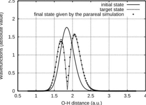
monotonic convergent algorithm in Eqns (9)-(11) (with δ = 0.25 = η, δ = 1 = η and δ = 2, η = 0) in each (nonlinear) propagation the parareal scheme was employed, with only one parareal iteration per evolution equation. The results in Fig 3 (δ = 1 = η) show that a good overlap with the objective operator is reached Our actual implementation is not yet parallel, but we estimate that a parallel imple-mentation would yield in an overall gain factor (in real time required to solve the problem) of the order of 5.
For this case other choices for the parameters δ and η give the expected behavior [6]: for in-stance δ = 0.25 = η converges slower than δ = 1.0 = η that is turn converges slower than δ = 2, η = 0. For other cases not re-ported here we could identify some choices of time steps for which the setting δ = 0.25 = η converges but not δ = 1.0 = η; the explana-tion may be in the high nonlinearity of the equations Eqns (9)-(11) implied by the choice δ = 1.0 = η, this nonlinearity being reduced in the case δ = 0.25 = η.
5 Conclusion and perspectives In an effort to introduce the parallel in time discretization for the simulation of quantum
0 0.5 1 1.5 2 2.5 0.5 1 1.5 2 2.5 3 3.5 4
Wavefunctions (absolute value)
O-H distance (a.u.) initial state target state final state given by the parareal simulation
Figure 3: Plotting |ψ0|, |ψT| and |ψ(x, T )|
ob-tained with the controlled field. Com-plete overlap with the target is ob-served for the parareal scheme solved with the algorithm in Eqns (9)-(11) with δ = 1 = η.
control problems we have presented here our preliminary studies that show the feasibility of the parareal implementations. Much work is still to be done in the direction of choosing more efficient coarse propagators and also in the adaptation of the overall scheme to equa-tions (like those of the quantum control) where conservation laws are present. This results, even if encouraging, still need to be improved in order to gain in reliability and stability. The natural continuation would be the search for ef-ficient entangled control-parareal formulation as in [5] in order to combine the parareal up-date directly with the control iterations.
Acknowledgments. It is a pleasure to
ac-knowledge helpful discussions that we had on this topic with Prof. O. Pironneau ( Jacques-Louis Lions Laboratory, Paris) and W. Zhu from Princeton Univeristy.
References
[1] A. Assion et al. Control of chemical
reac-tions by feedback-optimized phase-shaped fem-tosecond laser pulses. Science, 282:919–922, 1998.
[2] L.Baffico, S.Bernard, Y.Maday,
G.Turinici and G.Zerah Parallel in time
molecular dynamics simulations, in prepara-tion
[3] G. Bal and Y. Maday, “A “parareal” time
discretization for the non-linear PDE’s with application to the pricing of an American put”, in Proceedings of the workshop on domain De-composition, LNCSE Series, Springer Verlag, Zurich, 2001
[4] J.-L. Lions, Y. Maday and G. Turinici, A
“parareal” in time discretization of PDE’s, C. R. Acad. Sci. Paris, S´er. I, Math. 332 (2001), no. 7, 661–668
[5] Y.Maday, G.Turinici A parareal in time
procedure for the control of partial differential
equations, C. R. Acad. Sci. Paris, S´er. I, Math.
(2002), in press
[6] Y. Maday and G. Turinici New
formu-lations of monotonically convergent quantum
control algorithms, in preparation.
[7] S.Shi, A. Woody, and H.Rabitz,
Opti-mal control of selective vibrational excitation
in harmonic linear chain molecules , J.Chem
Phys. 88(1988), p.6870
[8] W. Zhu, J. Botina and H. Rabitz Rapidly
convergent iteration methods for quantum op-timal control of population, J. Chem. Phys. 108(1998), 1953
[9] W. Zhu and H.Rabitz A rapid
monitoni-cally convergent iteration algorithm for quan-tum optimal control over the expectation value of a positive definite operator, J.Chem.Phys, 109 (2), p385-391, 1998