HAL Id: hal-01418915
https://hal.archives-ouvertes.fr/hal-01418915
Submitted on 17 Dec 2016
HAL is a multi-disciplinary open access
archive for the deposit and dissemination of
sci-entific research documents, whether they are
pub-lished or not. The documents may come from
teaching and research institutions in France or
abroad, or from public or private research centers.
L’archive ouverte pluridisciplinaire HAL, est
destinée au dépôt et à la diffusion de documents
scientifiques de niveau recherche, publiés ou non,
émanant des établissements d’enseignement et de
recherche français ou étrangers, des laboratoires
publics ou privés.
A Logic of Singly Indexed Arrays
Peter Habermehl, Radu Iosif, Tomáš Vojnar
To cite this version:
Peter Habermehl, Radu Iosif, Tomáš Vojnar. A Logic of Singly Indexed Arrays. Logic for
Program-ming, Artificial Intelligence, and Reasoning, 15th International Conference, LPAR 2008„ Nov 2008,
Doha, Qatar. �10.1007/978-3-540-89439-1_39�. �hal-01418915�
A Logic of Singly Indexed Arrays
!
Peter Habermehl1, Radu Iosif2, and Tom´aˇs Vojnar3
1 LSV, ENS Cachan, CNRS, INRIA; 61 av. du Pr´esident Wilson, F-94230 Cachan, France
and LIAFA, University Paris 7, Case 7014, 75205 Paris Cedex 13, [email protected]
2 VERIMAG, CNRS, 2 av. de Vignate, F-38610 Gi`eres, France, e-mail:[email protected]
3 FIT BUT, Boˇzetˇechova 2, CZ-61266, Brno, Czech Republic, e-mail: [email protected]
Abstract. We present a logic interpreted over integer arrays, which allows
dif-ference bound comparisons between array elements situated within a constant sized window. We show that the satisfiability problem for the logic is undecidable for formulae with a quantifier prefix{∃,∀}∗∀∗∃∗∀∗. For formulae with quantifier prefixes in the∃∗∀∗fragment, decidability is established by an automata-theoretic
argument. For each formula in the∃∗∀∗ fragment, we can build a flat counter
automaton with difference bound transition rules (FCADBM) whose traces cor-respond to the models of the formula. The construction is modular, following the syntax of the formula. Decidability of the∃∗∀∗fragment of the logic is a conse-quence of the fact that reachability of a control state is decidable for FCADBM.
1 Introduction
Arrays are commonplace data structures in most programming languages. Reasoning about programs with arrays calls for expressive logics capable of encoding pre- and post-conditions as well as loop invariants. Moreover, in order to automate program ver-ification, one needs tractable logics whose satisfiability problems can be answered by efficient algorithms.
In this paper, we present a logic of integer arrays based on universally quanti-fied comparisons between array elements situated within a constant sized window, i.e., quantified boolean combinations of basic formulae of the form∀i . !(i) → a1[i + k1] −
a2[i + k2] ≤ m where ! is a positive boolean combination of bound and modulo con-straints on the index variable i, a1and a2are array symbols, and k1, k2, m∈ Z are inte-ger constants. Hence the name of Single Index Logic (SIL). Note that SIL can also be viewed as a fragment of Presburger arithmetic extended with uninterpreted functions mapping naturals to integers.
The main idea in defining the logic is that only one universally quantified index may be used on the right hand side of the implication within a basic formula. According to [10], this restriction is not a real limitation of the expressive power of the logic since a formula using two or more universally quantified variables in a difference bound constraint on array values can be equivalently written in the form above, by introducing fresh array symbols. This technique has been detailed in [10].
Working directly with singly-indexed formulae allows to devise a simple and ef-ficient decision procedure for the satisfiability problem of the∃∗∀∗fragment of SIL,
!The work was supported by the French Ministry of Research (RNTL project AVERILES),
the Czech Grant Agency (projects 102/07/0322, 102/05/H050), the Czech-French Barrande project MEB 020840, and the Czech Ministry of Education by project MSM 0021630528.
based on a modular translation of formulae into deterministic flat counter automata with difference bound transition rules (FCADBM). This is possible due to the fact that deterministic FCADBM are closed under union, intersection and complement, when considering their sets of traces.
The satisfiability problem for∃∗∀∗-SIL is thus reduced to checking reachability of a control state in an FCADBM. The latter problem has been shown to be decidable first in [6], by reduction to the satisfiability problem of Presburger arithmetic. Later on, the method described in [4] reduced this problem to checking satisfiability of a linear Diophantine system, leading to the implementation of the FLATA toolset [7].
Universally quantified formulae of the form∀i . !(i) → "(i) are a natural choice when reasoning about arrays as one usually tend to describe facts that must hold for all array elements (array invariants). A natural question is whether a more complex quantification scheme is possible, while preserving decidability. In this paper, we show that the satisfiability problem for the class of formulae with quantifier prefixes of the form∀∗∃∗∀∗is already undecidable, providing thus a formal reason for the choice of working with existentially quantified boolean combinations of universal basic formulae. The contribution of this paper is hence three-fold:
– we show that the satisfiability problem for the class of formulae with quantifier
prefixes of the form∀∗∃∗∀∗is undecidable,
– we define a class of counter automata that is closed under union, intersection and
complement of their sets of traces,
– we provide a decision procedure for the satisfiability problem within the fragment
of formulae with alternation depth of at most one, based on a modular, simple, and efficient translation of formulae into counter automata.
The practical usefulness of the SIL logic is shown by giving a number of examples of properties that are recurrent in programs handling array data structures.
Related Work. The saga of papers on logical theories of arrays starts with the seminal
paper [15], in which the read and write functions from/to arrays and their logical axioms were introduced. A decision procedure for the quantifier-free fragment of the theory of arrays was presented in [12]. Since then, various quantifier-free decidable logics on arrays have been considered—e.g., [17, 13, 11, 16, 1, 8].
In [5], an interesting logic, within the∃∗∀∗quantifier fragment, is developed. Unlike our decision procedure based on automata theory, the decision procedure of [5] is based on a model-theoretic observation, allowing to replace universal quantification by a finite conjunction. The decidability of their theory depends on the decidability of the base theory of array values. However, compared to our results, [5] does not allow modulo constraints (allowing to speak about periodicity in the array values) nor reasoning about array entries at a fixed distance (i.e., reasoning about a[i] and a[i+ k] for a constant k and a universally quantified index i). The authors of [5] give also interesting undecidability results for extensions of their logic. For example, they show that relating adjacent array values (a[i] and a[i + 1]), or having nested reads, leads to undecidability.
A restricted form of universal quantification within∃∗∀∗formulae is also allowed in [2], where decidability is obtained based on a small model property. Unlike [5] and our work, [2] allows a hierarchy-restricted form of array nesting. However, similar to the restrictions presented above, neither modulo constraints on indices, nor reasoning about array entries at a fixed distance are allowed. A similar restriction not allowing to
express properties of consecutive elements of arrays appears also in [3], where a quite general∃∗∀∗logic on multisets of elements with associated data values is considered.
The closest in spirit to the present paper is our previous work in [10]. There, we es-tablished decidability of formulae in the∃∗∀∗quantifier prefix class when references to adjacent array values (e.g., a[i] and a[i + 1]) are not used in disjunctive terms. However, there are two essential differences between this work and the one reported in [10].
On one hand, the basic propositions from [10], allowing multiple universally quanti-fied indices could not be translated directly into counter automata. This led to a complex elimination procedure based on introducing new array symbols, which produces singly-indexed formulae. However, the automata resulting from this procedure are not closed under complement. Therefore, negation had to be eliminated prior to reducing the for-mula to the singly-indexed form, causing further complexity. In the present work, we start directly with singly-indexed formulae, convert them into automata, and compose the automata directly using boolean operators (union, intersection, complement).
On the other hand, using universally quantified array property formulae as building blocks for the formulae, although intuitive, is not formally justified in [10]. Here, we prove that alternating quantifiers to a depth more than two leads to undecidability.
Roadmap. The paper is organised as follows. Section 2 introduces the necessary
no-tions on counter automata and defines the class of FCADBM. Section 3 defines the logic SIL. Next, Section 4 gives the undecidability result for the entire logic, while Section 5 proves decidability of the satisfiability for the∃∗∀∗fragment, by translation to deterministic FCADBM. Finally, Section 6 presents some concluding remarks. For space reasons, most of the proofs are deferred to [9].
2 Counter Automata
Given a formula #, we denote by FV (#) the set of its free variables. If we denote a formula as #(x1, ..., xn), we assume FV(#) ⊆ {x1, ..., xn}. For #(x), we denote by
#[t/x] the formula in which each free occurrence of x is replaced by a term t. Given a formula #, we denote by|= # the fact that # is logically valid, i.e., it holds in every structure corresponding to its signature.
A difference bound matrix (DBM) formula is a conjunction of inequalities of the forms (1) x− y ≤ c, (2) x ≤ c, or (3) x ≥ c, where c ∈ Z is a constant. We denote by* (true) the empty DBM. It is well-known that the negation of a DBM formula is equivalent to a finite disjunction of pairwise disjoint DBM formulae since, e.g.,¬(x −
y≤ c) ⇐⇒ y − x ≤ −c − 1 and ¬(x ≤ c) ⇐⇒ x ≥ c + 1. In particular, the negation of
* is the empty disjunction, denoted as ⊥ (false).
A counter automaton (CA) is a tuple A =.x,Q,I,−→,F/ where:
– x is a finite set of counters ranging overZ,
– Q is a finite set of control states, – I⊆ Q is a set of initial states,
– −→ is a transition relation given by a set of rules q−−−−→ q#(x,x0) 0where # is an arithmetic formula relating current values of counters x to their future values x0= {x0| x ∈ x},
– F⊆ Q is a set of final states.
A configuration of a counter automaton A is a pair (q, $) where q∈ Q is a control state, and $ : x→ Z is a valuation of the counters in x. For a configuration c = (q,$), we
designate by val(c) = $ the valuation of the counters in c. A configuration (q0, $0) is an
immediate successor of (q, $) if and only if A has a transition rule q−−−−→ q#(x,x0) 0such that |= #($(x),$0(x0)). A configuration c is a successor of another configuration c0 if and only if there exists a finite sequence of configurations c = c1c2. . . cn= c0such that, for
all 1≤ i < n, ci+1 is an immediate successor of ci. Given two control states q, q0∈ Q,
a run of A from q to q0is a finite sequence of configurations c1c2. . . cnwith c1= (q,$),
cn= (q0, $0) for some valuations $,$0: x→ Z, and ci+1is an immediate successor of ci,
for all 1≤ i < n. Let
R
(A) denote the set of runs of A from some initial state q0∈ I to some final state qf ∈ F, and Tr(A) = {val(c1)val(c2)...val(cn) | c1c2. . . cn∈R
(A)}be its set of valuation traces. If z⊆ x is a subset of the counters of A and $ : x → Z is a valuation of its counters, let $↓zbe the restriction of $ to the counters in z. If c = (q, $)
is a configuration of A, we denote c↓z= (q,$ ↓z) and Tr(A) ↓z= {val(c1) ↓zval(c2) ↓z
. . . val(cn)↓z | c1c2. . . cn∈
R
(A)}.A counter z∈ x is called a parameter of A if and only if, for each % = $1. . . $n∈
Tr(A), we have $1(z) = ... = $n(z), in other words the value of the counter does not
change during any run of A.
A control path in a counter automaton A is a finite sequence q1q2. . . qnof control
states such that, for all 1≤ i < n, there exists a transition rule qi−→ q#i i+1. A cycle is
a control path starting and ending in the same control state. An elementary cycle is a cycle in which each state appears only once, except for the first one, which appears both at the beginning and at the end. A counter automaton is said to be flat iff each control state belongs to at most one elementary cycle.
A counter automaton A is said to be deterministic if and only if (1) it has exactly one initial state, and (2) for each pair of transition rules with the same source state q −→ q# 0 and q−→ q& 00, we have|= ¬(# ∧ &). It is easy to prove that, given a deterministic counter automaton A, for each sequence of valuations $1$2. . . $n∈ Tr(A) there exists exactly
one control path q1q2. . . qnsuch that (q0, $1)(q1, $2)... (qn−1, $n) ∈
R
(A).2.1 Flat Counter Automata with DBM Transition Rules
In the rest of the paper, we use the class of flat counter automata with DBM transition
rules (FCADBM). They are defined to be flat counter automata where each transition
in a cycle is labelled by a DBM formula and each transition not in a cycle is labelled by a conjunction of a DBM formula with a (possibly empty) conjunction of modulo constraints on parameters of the form z≡st where 0≤ t < s.
An extension of this class has been studied in [10]. Using results of [6, 4], [10] shows that, given a CA A =.x,Q,I,−→,F/ in the class it considers and a pair of control states q, q0∈ Q, the set Vq,q0= {($,$0) ∈ (x 4→ Z)2| A has a run from (q,$) to (q0, $0)}
is Presburger-definable. As an immediate consequence, the emptiness problem for A, i.e., Tr(A)= /0, is decidable.?
Theorem 1. The emptiness problem for FCADBM is decidable.
In this section, we show that deterministic FCADBM are closed under union, inter-section, and complement of their sets of traces. Let Ai= .x,Qi,{q0i},→i, Fi/, i = 1,2,
be two deterministic FCADBM with the same set of counters. Note that this is not a re-striction as one can add unrestricted counters without changing the behaviour of a CA. We first show closure under intersection by defining the CA A1⊗ A2= .x,Q1× Q2, {(q01, q02)},→, F1× F2/ where (q1, q2)−→ (q# 01, q02) ⇐⇒ q1
&1
→1q01, q2 &2
→2q02, and |= # ↔ &1∧ &1. The next lemma proves the correctness of our construction.
Lemma 1. For any two deterministic FCADBM Ai = .x,Qi,{qi0},→i, Fi/, i = 1,2,
A1⊗ A2is a deterministic FCADBM, and Tr(A1⊗ A2) = Tr(A1) ∩ Tr(A2).
Let A =.x,Q,I,−→,F/ be a deterministic FCADBM. Then we define A = .x,Q ∪ {qs},I,→0, (Q\ F)∪{qs}/ where qs:∈ Q is a fresh sink state. The transition relation →0
is defined as follows. For a control state q∈ Q, let OA(q) =W q−→#q0#.
4Then, we have:
– qs→*0qs, q→#0q0for each q→ q# 0, and
– q→&i0qs, for all 1≤ i ≤ k, where &iare (unique) conjunctions of DBMs and modulo constraints5such that|= ¬OA(q) ↔Wi=1k &iand|= ¬(&i∧&j) for i := j, 1 ≤ i, j ≤ k.
Flatness of A is a consequence of the fact that the only cycle of A, which did not exist in A, is the self-loop around qs. That is, the newly added transitions do not create new
cycles. It is immediate to see that A is deterministic whenever A is. The following lemma formalises correctness of the complement construction, proving thus that deterministic FCADBM are effectively closed under union6, intersection, and complement of their sets of traces.
Lemma 2. Given a deterministic FCADBM A =.x,Q,{q0},→,F/, for any finite
se-quence of valuations %∈ (x 4→ Z)∗, we have %∈ Tr(A) if and only if % :∈ Tr(A).
3 A Logic of Integer Arrays
3.1 Syntax
We consider three types of variables. The array-bound variables (k, l) appear within the bounds that define the intervals in which some property is required to hold. Let BVar denote the set of bound variables. The index (i, j) and array (a, b) variables are used in array terms. Let IVar denote the set of integer variables and AVar denote the set of
array variables. All variable sets are supposed to be finite and of known cardinality.
Fig. 1 shows the syntax of the Single Index Logic SIL. The term|a| denotes the length of an array variable a. We use the symbol* to denote the boolean value true. In the following, we will write f ≤ i ≤ g instead of f ≤ i ∧ i ≤ g, i < f instead of
i≤ f − 1, i = f instead of f ≤ i ≤ f , #1∨ #2instead of¬(¬#1∧ ¬#2), and ∀i . "(i) instead of∀i . * → "(i). If "1(k1),...,"n(kn) are array-bound terms with free variables
k1, . . . , kn∈ BVar, respectively, we write any DBM formula # on terms a1["1],...,an["n],
as a shorthand for (Vnk=1∀ j . j = "k→ ak[ j] = lk) ∧ #[l1/a1["1],...,ln/an["n]], where
l1, . . . , lnare fresh array-bound variables.
4If q has no immediate successors, then O
A(q) is false by default.
5The negation of z≡
st with t < s is equivalent toWt0∈{0,...,s−1}\{t}z≡st0.
6The FCADBM whose set of traces is the union of the sets of traces of two given FCADBM
n, m, p . . .∈ Z constants
k, l, . . . ∈ BVar array-bound variables
i, j, . . . ∈ IVar index variables
a, b, . . . ∈ AVar array variables
∼ ∈ {≤,≥}
B := n| k + n | |a| + n array-bound terms
G :=* | i − j ≤ n | i ≤ B | B ≤ i | i ≡st| G ∧ G | G ∨ G guard expressions (0 ≤ t < s)
V := a[i + n]∼ B | a[i + n] − b[i + m] ∼ p |
i− a[i + n] ∼ m | V ∧V value expressions
C := B∼ n | B − B ≤ n | B ≡st array-bound constraints (0≤ t < s)
P :=∀i . G → V array properties
F := P| C | ¬F | F ∧ F | F ∨ F | ∃i . F formulae
Fig. 1. Syntax of the Single Index Logic
For reasons that will be made clear later on, we allow only one index variable to oc-cur within the right hand side of the implication in an array property formula∀i . ! → ", i.e., we require FV (")∩ IVar = {i}. Hence the name Single Index Logic (SIL). Note that this does not restrict the expressive power w.r.t. the logic considered in [10]. One can always circumvent this restriction by using the method from [10] based on adding new array symbols together with a transitive (increasing, decreasing, or constant) con-straint on their adjacent values. This way a relation between arbitrarily distant entries
a[i] and b[ j] is decomposed into a sequence of relations between neighbouring entries
of a, b, and entries of the auxiliary arrays. However this transformation would greatly complicate the decision procedure, hence we prefer to avoid it here.
Notice also that one can compare an array value with an array-bound variable, or with another array value on the right hand side of an implication in an array property formula∀i . ! → ", but one cannot relate two or more array values with array-bound parameters in the same expression. Allowing more complex comparisons between array values would impact upon the decidability result reported in Section 5. For the same reason, disjunctive terms are not allowed on the right hand side of implications in array properties: Intuitivelly, allowing disjunctions in value expressions would allow one to code 2-counter machines with possibly nested loops (as shown already in [10]).
Let " be a value expression written in the syntax of Fig. 1 (starting with the V non-terminal). Let
B
(") be the formula defined inductively on the structure of " as follows:–
B
(a[i + n] ≤ B) =B
(B ≤ a[i + n]) = 0 ≤ i + n < |a| –B
(i − a[i + n] ≤ m) =B
(a[i + n] − i ≤ m) = 0 ≤ i + n < |a| –B
(a[i + n] − b[i + m] ≤ p) = 0 ≤ i + n < |a| ∧ 0 ≤ i + m < |b| –B
("1∧ "2) =B
("1) ∧B
("2)Intuitively,
B
(") is the conjunction of all sanity conditions needed in order for the array accesses in " to occur within proper bounds.3.2 Semantics
Let us fix AVar ={a1, a2, . . . , ak} as the set of array variables for the rest of this section.
an integer value with every free integer variable, and µ : AVar→ Z∗associates a finite
sequence of integers with every array symbol a∈ AVar. If % ∈ Z∗is such a sequence, we denote by|%| its length and by %iits i-th element.
By
I
',µ(t), we denote the value of the term t under the valuation .',µ/. The semantics of a formula # is defined in terms of the forcing relation|= as follows:I
',µ(|a|) = |µ(a)|I
',µ(a[i + n]) = µ(a)'(i)+n.',µ/ |= a[i + n] ≤ B ⇐⇒
I
',µ(a[i + n]) ≤ '(B) .',µ/ |= A1− A2≤ n ⇐⇒I
',µ(A1) −I
',µ(A2) ≤ n.',µ/ |= ∀i . G → V ⇐⇒ ∀ n ∈ Z . .'[i ← n],µ/ |= G ∧
B
(V) → V .',µ/ |= ∃i . F ⇐⇒ .'[i ← n],µ/ |= F for some n ∈ NNotice that the semantics of an array property formula∀i . G → V ignores all values of i for which the array accesses of V are undefined since we consider only the values of
i fromZ that satisfy the safety assumption
B
(V). For space reasons, we do not give herea full definition of the semantics. However, the missing rules are standard in first-order arithmetic. A model of a SIL formula #(k, a) is a valuation.',µ/ such that the formula obtained by interpreting each variable k∈ k as '(k) and each array variable a ∈ a as
µ(a) is logically valid:.',µ/ |= #. We define [[#]] = {.',µ/ | .',µ/ |= #}. A formula is
said to be:
– satisfiable if and only if [[#]]:= /0, and
– valid if and only if [[#]] = (BVar∪ IVar → Z⊥) × (AVar → Z∗)
With these definitions, the satisfiability problem asks, given a formula # if it has at least one model. Without losing generality, for the satisfiability problem, we can assume that the quantifier prefix of # (in prenex normal form) does not start with∃. Dually, the
validity problem asks whether a given formula holds on every possible model.
Symmet-rically, for the validity problem, one can assume w.l.o.g. that the quantifier prefix of the given formula does not start with∀.
3.3 Examples
We now illustrate the syntax, semantics, and use of the logic SIL on a number of ex-amples. For instance, the formula∀i . a[i] = 0 is satisfied by all functions µ mapping a to a finite sequence of 0’s, i.e., µ(a)∈ 0∗. It is semantically equivalent to∀i . 0 ≤ i < |a| → a[i] = 0, in which the range of i has been made explicit.
The formula∀i . 0 ≤ i < k → a[i] = 0 is satisfied by all pairs .',µ/ where µ maps a to a sequence whose first '(k) elements (if they exist) are 0, i.e., µ(a)∈ {0n| 1 ≤ n <
'(k)} ∪ 0'(k)Z∗. It is semantically equivalent to∀i . 0 ≤ i < min(|a|,k) → a[i] = 0. The capability of SIL to relate array entries at fixed distances (missing in many decidable logics such as those considered in [2, 5, 3]) is illustrated on a bigger example below. The modulo constraints on the index variables can then be used to state periodic facts. For instance, the formula∀i . i ≡20→ a[i] = 0 ∧ ∀i . i ≡21→ a[i] = 1 describes the set of arrays a in which the elements on even positions have the value 0, and the elements on odd positions have the value 1.
The logic SIL also allows direct comparisons between indices and values. For in-stance, the formula∀i . a[i] = i + 1 is satisfied by all arrays a which are of the form
1234 . . . . Alternatively, this can be specified as a[0] = 1∧ ∀i . a[i + 1] = a[i]+ 1 where
a[0] = 1 is a shorthand for∀i . i = 0 → a[i] = 1. Further, the set of arrays in which the
value at position n is between zero and n can be specified by writing∀i . 0 ≤ a[i] < i, which cannot be described without an explicit comparison between indices and values (unless a comparison with an additional array describing the sequence 1234 . . . is used).
Checking verification conditions for array manipulating programs. The decision
proce-dure for checking satisfiability of SIL formulae, described later on, can be used for dis-charging verification conditions of various interesting array-manipulating procedures. As a concrete example, let us consider the procedure for an in-situ left rotation of arrays, given below. We annotate the procedure (using double braces) with a pre-condition, post-condition, and a loop invariant. We distinguish below logical variables from pro-gram variables (typeset in print). The variable a0 is a logical variable that relates the initial values of the array a with the values after the rotation.
{{ |a| = |a0| ∧∀ j.a[ j] = a0[ j] }} x=a[0];
for (i=0; i <|a|-1; i++)
{{ x = a0[0] ∧ ∀ j.0 ≤ j < i → a[ j] = a0[ j + 1] ∧ ∀ j.i ≤ j < |a| → a[ j] = a0[ j] }} a[i]=a[i+1];
a[|a|-1]=x;
{{ a[|a| − 1] = a0[0] ∧ ∀ j.0 ≤ j < |a| − 1 → a[ j] = a0[ j + 1]) }}
To check (partial) correctness of the procedure, one needs to check three verifica-tion condiverifica-tions out of which we discuss one here (the others are similar). Namely, we consider checking the loop invariant, which requires checking validity of the formula:
x= a0[0] ∧ ∀ j.0 ≤ j < i → a[ j] = a0[ j + 1] ∧ ∀ j.i ≤ j < |a| → a[ j] = a0[ j] ∧ i < |a| − 1 ∧ |a0| = |a| ∧ i0= i + 1 ∧ x0= x ∧ a0[i] = a[i + 1] ∧ ∀ j. j := i → a0[ j] = a[ j]
−→
x0= a0[0] ∧ ∀ j.0 ≤ j < i0→ a0[ j] = a0[ j + 1] ∧ ∀ j.i0≤ j < |a0| → a0[ j] = a0[ j] Primed variables denote the values of program variables after one iteration of the loop. Checking validity of this formula amounts to checking that its negation is unsatisfiable. The latter condition is expressible in the decidable fragment of SIL. Note that the con-ditions used above refer to adjacent array positions, which could not be expressed in the logics defined in [2, 5, 3].
4 Undecidability of the Logic SIL
In this section, we show that the satisfiability problem for the∀∗∃∗∀∗fragment of SIL is undecidable, by reducing from the Hilbert’s Tenth Problem [14]. In the following, Sec-tion 5 proves the decidability of the satisfiability problem for the fragment of boolean combinations of universally quantified array property formulae—the satisfiability of the ∀∗fragment is proven. Since the leading existential prefix is irrelevant when one speaks about satisfiability, referring either to∀∗∃∗∀∗or to∃∗∀∗∃∗∀∗makes no difference in this case. However, the question concerning the validity problem for the∃∗∀∗fragment of SIL is still open.
First, we show that multiplication and addition of strictly positive integers can be encoded using formulae of∀∗∃∗∀∗-SIL. Let x, y, z∈ N, with z > 0. We define:
#1( j) : a2[ j] > 0 ∧ a3[ j] > 0 ∧ a1[ j + 1] = a1[ j] + 1 ∧ a2[ j + 1] = a2[ j] − 1 ∧ ∧ a3[ j + 1] = a3[ j]
#2( j) : a2[ j] = 0 ∧ a3[ j] > 0 ∧ a1[ j + 1] = a1[ j] ∧ a2[ j + 1] = y ∧ a3[ j + 1] = a3[ j] − 1 #x=yz(a1, a2, a3, n1, n2) : n1< n2∧ a1[n1] = 0 ∧ a2[n1] = y ∧ a3[n1] = z ∧ a1[n2] = x ∧
∧ a3[n2] = 0 ∧ ∀i.(n1≤ i < n2→ ∃ j.i ≤ j < n2∧ #2( j) ∧ ∀k.(i ≤ k < j → #1(k))) Notice that #x=yzis in the∀∗∃∗∀∗quantifier fragment of SIL.
Lemma 3. #x=yz(a1, a2, a3, n1, n2) is satisfiable if and only if x = yz.
Proof. We first suppose that x = yz and give a model of #x=yz(a1, a2, a3, n1, n2). We
choose n1= 0 and n2= (y+1)z. Then, we choose a1[n2] = x, a2[n2] = y and a3[n2] = 0. Furthermore, for all j such that 0≤ j < z and for all i such that 0 ≤ i ≤ y, we choose
a1[i + j(y + 1)] = i + jy, a2[i + j(y + 1)] = y − i and a3[i + j(y + 1)] = z − j. Then, it is
easy to check that this is a model of #x=yz(a1, a2, a3, n1, n2).
Let us consider now a model of #x=yz(a1, a2, a3, n1, n2). We show that this implies
x = yz. A model of n1< n2∧a1[n1] = 0∧a2[n1] = y∧a3[n1] = z∧a1[n2] = x∧a3[n2] = 0∧∀i.(n1≤ i < n2→ ∃ j.i ≤ j < n2∧#2( j)∧∀k.(i ≤ k < j → #1(k))) assigns values to
n1and n2and defines array values for a1, a2, and a3between bounds n1and n2. Clearly,
a1[n1] = 0, a2[n1] = y, a3[n1] = z, a1[n2] = x, and a3[n2] = 0. Due to their definition, #1( j) and #2( j) cannot be true at the same point j since |= #1( j) → a2[ j] > 0 and |= #2( j) → a2[ j] = 0.
Since the subformula∀i.(n1≤ i < n2→ ∃ j.i ≤ j < n2∧ #2( j) ∧ ∀k.(i ≤ k < j → #1(k))) holds, it is then clear that there exists points j1, . . . , jlwith l > 0 and n1≤ j1<
j2<··· < jl = n2− 1 such that #2( j) holds at all of these points. Furthermore, at all
intermediary points k not equal to one of the ji’s, #1(k) has to be true. This implies
that l must be equal to z (since #1(k) imposes a3[k + 1] = a3[k] whereas #2( j) imposes
a3[ j + 1] = a3[ j] − 1).
Let us examine the intermediary points between n1 and j1. Due to a1[n1] = 0,
a2[n1] = y, a3[n1] = z and #1(k) being true for all k such that n1≤ k < j1 as well as #2( j1) being true, we must have j1= y + n1, and, for all k such that n1< k≤ j1, we have a1[k] = k − n1, a2[k] = y − k + n1, and a3[k] = z. Furthermore, since #2( j1) is true, we have a1[ j1+ 1] = y, a2[ j1+ 1] = y, and a3[ j1+ 1] = z − 1. We can continue this reasoning with the intermediary points between j1and j2 and so on up to jl. At the
end we get a3[ jl+ 1] = 0 and a1[ jl+ 1] = a1[n2] = yl. Since l = z and a1[n2] = x, this
implies x = yz. >?
Next, we define:
#3( j) : a2[ j] > 0 ∧ a1[ j + 1] = a1[ j] + 1 ∧ a2[ j + 1] = a2[ j] − 1
#x=y+z(a1, a2, n1, n2) : n1< n2∧ a1[n1] = y ∧ a2[n1] = z ∧ a1[n2] = x ∧ a2[n2] = 0 ∧
Lemma 4. #x=y+z(a1, a2, n1, n2) is satisfiable if and only if x = y + z.
Proof. Similar to Lemma 3. >?
We are now ready to reduce from the Hilbert’s Tenth Problem [14]. Given a Dio-phantine system S, we construct a SIL formula (Swhich is satisfiable if and only if
the system has a solution. Without loss of generality, we can suppose that all variables in S range over strictly positive integers. Then S can be equivalently written as a sys-tem of equations of the form x = yz and x = y + z by introducing fresh variables. Let {x1, . . . , xk} be the variables of these equations. We enumerate separately all equations
of the form x = yz and those of the form x = y + z. Let nmbe the number of equations
of the form x = yz and nathe number of equations of the form x = y + z.
Let (Sbe the following SIL formula with three array symbols (a1, a2and a3):
∃x1. . .∃xk∃m11. . .∃m1nm+na∃m 2 1. . .∃m2nm+na nm+n^a−1 i=1 m2i < m1i+1∧ nm ^ i=1 #i∧ na ^ i=1 #0i
where the formulae #i and #0i are defined as follows: Let xi1= xi2xi3 be the i-th
mul-tiplicative equation. Then, #i= #xi1=xi2xi3(a1, a2, a3, m1i, m2i). Let xi1 = xi2+ xi3 be the
i-th additive equation. Then, #0i= #xi1=xi2+xi3(a1, a2, m1nm+i, m2nm+i).
Lemma 5. A Diophantine system S has a solution if and only if the corresponding formula (Sis satisfiable.
Proof. The Diophantine system S is equivalently written as a conjunction of equations
of the form x = yz and x = y + z using variables{x1, . . . , xk}. Then, the Diophantine
system has a solution if and only if all equations of the form x = yz and x = y + z have a common solution. Since all pairs m1i and m2i denote disjoint intervals and using Lemmas 3 and 4, we have that all equations of the form x = yz and x = y + z have
a common solution if and only if (Sis satisfiable. >?
5 Decidability of the Satisfiability Problem for
∃
∗∀
∗-SIL
We show that the set of models of a boolean combination # of universally quantified ar-ray property formulae of SIL corresponds to the set of runs of an FCADBM A#, defined inductively on the structure of the formula. More precisely, each array variable in # has a corresponding counter in A#, and given any model of # that associates integer values to all array entries, A#has a run in which the values of the counters at different points of the run match the values of the array entries at corresponding positions in the model. Since the emptiness problem is decidable for FCADBM, this leads to decidability of the satisfiability problem for∃∗∀∗-SIL (or equivalently, for∀∗-SIL).
5.1 Normalisation
Before describing the translation of∃∗∀∗-SIL formulae into counter automata, we need to perform a simple normalisation step. Let #(k, a) be a SIL formula in the∃∗∀∗ frag-ment i.e., an existentially quantified boolean combination of (1) DBM conditions or
modulo constraints on array-bound variables k and array length terms|a|, a ∈ a, and (2) array properties of the form∀i . !(i,k,|a|) → "(i,k,a)7. Without losing generality, we assume that the sanity condition
B
(") is explicitly conjoined to the guard of every array property i.e., each array property is of the form∀i . ! ∧B
(") → ".A guard expression is a conjunction of array-bound expressions i∼ ", ∼ ∈ {≤,≥}, or modulo constraints i≡st where " is a an array bound term, and s,t∈ N such that
0≤ t < s. For a guard ! and an integer constant c ∈ Z, we denote by ! + c the guard obtained by replacing each array-bound expression i∼ b by i ∼ b + c and each modulo constraint i≡st by i≡st0where 0≤ t0< s and t0≡st + c.
The normalisation consists in performing the following steps in succession: 1. Replace each array property subformula∀i . Wj!j→Vk"kby the equivalent
con-junctionVj,k∀i . !j→ "kwhere !jare guard expressions and "kare either a[i+ n]∼
", a[i + n]− b[i + m] ∼ p, or i − a[i + n] ∼ m, where m,n, p ∈ Z, ∼∈ {≤,≥} and " is an array bound term.
2. Simplify each newly obtained array property subformula as follows: ∀i . ! → a[i + n] ∼ " ! ∀i . ! + n → a[i] ∼ "
∀i . ! → i − a[i + n] ∼ m ! ∀i . ! + n → i − a[i] ∼ m + n
∀i . ! → a[i + n] − b[i + m] ∼ p ! ∀i . ! + n → a[i] − b[i + m − n] ∼ p if m ≥ n ∀i . ! → a[i + n] − b[i + m] ∼ p ! ∀i . ! + m → b[i] − a[i + n − m]∼− p if m < n where:
– ∼∈ {≤,≥} and ∼ is ≥ (≤) if ∼ is ≤ (≥), respectively, and
– " is an array-bound term, and m, n, p∈ Z.
3. For each array property & :∀i . !(i) → "(i), let B&= {b1, . . . , bn} be the set of
array-bound terms occurring in !. Then replace & by the disjunctionW1≤i, j≤nV1≤k≤nbi≤
bk≤ bj∧ & (one considers all possible cases of minimal and maximal values for
array-bound terms), and simplify all subformulae of the form Vji≤ bj(Vji≥ bj)
from ! to exactly one upper (lower) bound, according to the current conjunctive clause. If the lower and upper bound that appear in ! are inconsistent with the chosen minimal and maximal value added by the transformation to & (i.e., the lower bound is assumed to be bigger than the upper one), we replace & in the concerned conjunctive clause by* as it is trivially satisfied.
4. Rewrite each conjunctionVji≡sj tjoccurring within the guards of array property
formulae intoVji≡SSs·tjj where S is the least common multiple of sj, and simplify
the conjunction either to false (in which case the array property subformula is vac-uously true), or to a formula i≡St. In case there is no modulo constraint within
a guard, for uniformity reasons, conjoin the guard with the constraint i≡10.
7An array property formula with more than one universally quantified index
vari-able occurring in the guard can be equivalently written as an array property for-mula whose guard has exactly one universally quantified index variable. Indeed, a formula of the form ∀i1, . . . , in . !(i1, . . . , in, k,|a|) → "(i1, k, a) is equivalent to
∀i1 . ((∃i2, . . . , in . !(i1, . . . , in, k,|a|)) → "(i1, k, a)) and then the existential quantifiers in
(∃i2, . . ., in . !(i1, . . . , in, k,|a|)) can be eliminated possibly adding modulo constraints on k,
5. Transform each array property subformula of the form
∀i . f ≤ i ≤ g ∧ i ≡st −→ a[i] − b[i + m] ∼ n
where m > 1, n∈ Z, and 0 ≤ t < s into the following conjunction: ∀i . f ≤ i ≤ g ∧ i ≡st −→ a[i] − )1[i + 1] ∼ 0 ∧
Vm−2
j=1∀i. f + j ≤ i ≤ g + j ∧ i ≡s(t + j) mod s −→ )j[i] − )j+1[i + 1] ∼ 0 ∧
∀i . f + m − 1 ≤ i ≤ g + m − 1 ∧ i ≡s(t + m − 1) mod s −→ )m−1[i] − b[i + 1] ∼ n
where )1, )2, . . . , )m−1are fresh array variables. Figure 2 depicts this transformation for∼=≤ – the case ∼=≥ is similar.
.. . g 0 0 0 0 0 0 0 0 f a )1 )2 b f + m )m−1 n n n n g + m
Fig. 2. Adding fresh array variables to array property formulae ∀i . f ≤ i ∧ i ≤ g ∧ i ≡st→
a[i]− b[i + m] ≤ n
The result of the normalisation step is a boolean combination of (1) DBM conditions or modulo constraints on array-bound variables k and array length terms|a|, a ∈ a and (2) array properties of the following form:
∀i . f ≤ i ≤ g ∧ i ≡st→ "
where f and g are array-bound terms, s,t∈ N, 0 ≤ s < t, and " is one of the following: (1) a[i] ∼ ", (2) i − a[i] ∼ n, (3) a[i] − b[i + 1] ∼ n
where∼∈ {≤,≥}, n ∈ Z, and " is an array-bound term.
We need the following definition to state the normal form lemma. If X⊆ AVar is a set of array variables, then µ↓Xrepresents the restriction of µ : AVar→ Z∗to the
vari-ables in X. For a formula # of SIL, we denote by [[#]]↓X the set{.',µ↓X/ | .',µ/ |= #}.
Lemma 6. Let #(k, a) be a formula of∃∗∀∗-SIL and *(k, a, t) be the formula obtained
from # by normalisation where t is the set of fresh array variables added during nor-malisation. Then we have [[#]] = [[*]]↓a.
5.2 Translating Normalised Formulae into FCADBM.
Let #(k, a) be an∃∗∀∗-SIL formula that is already normalised as in the previous. The automaton encoding the models of # is in fact a product
A
#= A#⊗ Atick, where A# is defined inductively on the structure of #, and Atickis a generic FCADBM, definednext. Both A#and Atick(and, implicitly
A
#) work with the set of counters x ={xk| k ∈– xkand x|a|are parameters corresponding to array-bound variables, i.e., their values do not change during the runs of
A
#,– xaare counters corresponding to the array symbols, and
– xtickis a special counter that is initialised to zero and incremented by each transition.
The main intuition behind the automata construction is that, for each model.',µ/ of #, there exists a run of
A
#such that, for each array symbol a∈ a, the value µ(a)nequalsthe value of xa when xtick equals n, for all 0≤ n < |a|. The reason behind defining
A
#as the product of A#and Atickis that the use of negation within #, which involvescomplementation on the automata level, may not affect the flow of ticks, just the way they are dealt with within the guards. For this reason, A#can only read x), while Atickis
the one updating it.
Formally, let Atick= .x,{q0, qtick},{q0},→tick,{qtick}/, where
q0
xtick=0 ∧ x0tick=xtick+1 ∧Vk∈kx0k=xk∧Va∈ax0|a|=x|a|
−−−−−−−−−−−−−−−−−−−−−−−−−−−−−−−→ qtick
and
qtick x0
tick=xtick+1 ∧Vk∈kx0k=xk∧Va∈ax0|a|=x|a|
−−−−−−−−−−−−−−−−−−−−−−−−−→ qtick
are the only transitions rules. The construction of A#is recursive on the structure of #:
– if # is a DBM constraint or modulo constraint + on array-bound terms, let A#=
.x,{q0, q1},{q0},−→,{q1}/ where the transitions rules are q1−→ q* 1and q0−→ q+ 1, and + is obtained from the constraint + by replacing all occurrences of k∈ k by xk,
and all occurrences of|a|, a ∈ a, by x|a|.
– if # =¬&, let A#= A&,
– if # = &1∧ &2, let A#= A&1⊗ A&2,
– if # = &1∨ &2, let A#= A&1⊗ A&2.
– if # is an array property, A# is defined below, according to the type of the value
expression occurring on the right hand side of the implication.
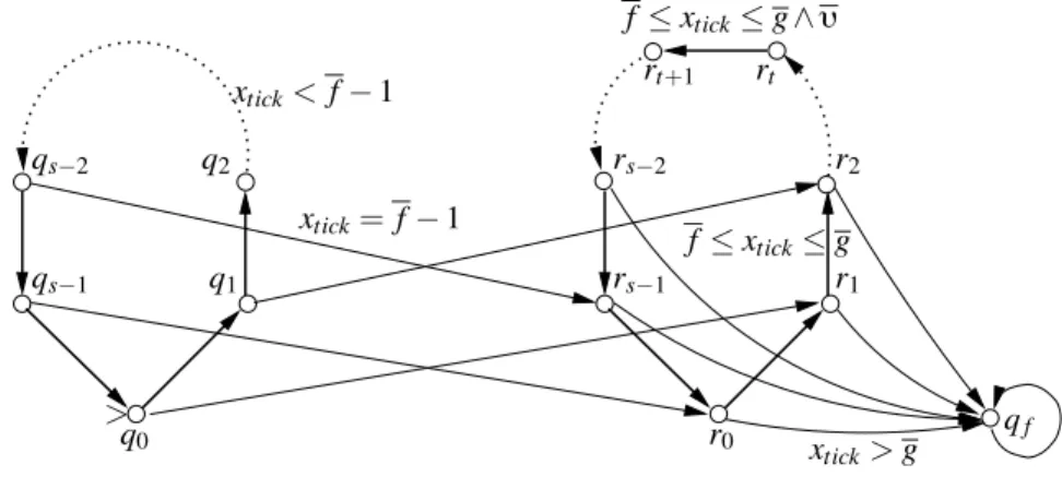
Let # :∀i . f ≤ i ≤ g ∧ i ≡st→ " be an array property subformula after
normal-isation. Figure 3 gives the counter automaton A#for such a subformula. The formal definition of A#= .x,Q,I,−→,F/ follows:
– Q ={qi| 0 ≤ i < s} ∪ {ri| 0 ≤ i < s} ∪{ qf}, I = {q0}, and F = {qf}.
– the transition rules of A#are as follows, for all 0≤ i < s:
qi−−−−−−→ q(i+1) mod sxtick< f−1 qi−−−−−−→ r(i+1) mod sxtick= f −1
ri−−−−−−→ r(i+1) mod sf≤xtick≤g if i:= t rt−−−−−−−−→ r(t+1) mod s"∧ f ≤xtick≤g
ri xtick>g −−−−→ qf qf −→ q* f q0 xtick=0 ∧ " ∧ f ≤xtick≤g −−−−−−−−−−−−−−→ r1 mod sif t = 0 q0 xtick=0 ∧ f ≤xtick≤g −−−−−−−−−−−→ r1 mod sif t:= 0 Here " is defined by:
• "= x, a∼ " if " is a[i] ∼ " where " is obtained from " by replacing each
occur-rence of k∈ k by xkand each occurrence of|a| by x|a|, a∈ a,
• "= x, tick− xa∼ n if " is i − a[i] ∼ n, and
• "= x, a− x0b∼ n if " is a[i] − b[i + 1] ∼ n.
Further, f (g) are obtained from f (g) by replacing each k∈ k by xkand each|a|,
a∈ a, by x|a|, respectively.
Notice that A#is always deterministic. This is because the automata for array prop-erty formulae are deterministic in the use of the xtick counter, complementation
pre-serves determinism, and composition of two deterministic FCADBM results in a deter-ministic FCADBM. > rs−2 r2 r1 rs−1 r0 q0 qf qs−2 q2 qs−1 q1 xtick< f− 1 f ≤ xtick≤ g ∧ " xtick> g xtick= f − 1 f≤ xtick≤ g rt rt+1
Fig. 3. The FCADBM for the formula∀i . f ≤ i ≤ g ∧ i ≡st→ "
Let #(k, a) be a normalised∃∗∀∗-SIL formula, and
A
#= A#⊗Atickbe thedetermin-istic FCADBM whose construction was given in the previous. We define the following relation between valuations.',µ/ ∈ [[#]] and traces % ∈ Tr(
A
#), denoted .',µ/ ≡ %, iff:1. for all k∈ k, '(k) = %0(xk),
2. for all a∈ a, '(|a|) = %0(x|a|) = |µ(a)| ≤ |%| and µ(a)i= %i(xa), 0 ≤ i < |µ(a)|.
The following lemma establishes correctness of our construction:
Lemma 7. Let #(k, a) be a normalised∃∗∀∗-SIL formula, and
A
#be its correspondingFCADBM. Then for each valuation.',µ/ ∈ [[#]] there exist a trace % ∈ Tr(
A
#) such that .',µ/ ≡ %. Dually, for each trace % ∈ Tr(A
#) there exists a valuation .',µ/ ∈ [[#]] suchthat.',µ/ ≡ %.
Theorem 2. The satisfiability problem is decidable for the∃∗∀∗fragment of SIL.
Proof. Let #(k, a) be a formula of∃∗∀∗-SIL. By normalisation, we obtain a formula *(k, a, t) where t is the set of fresh array variables added during normalisation. Then, by Lemma 6, we have [[#]] = [[*]]↓a. To check satisfiability of #, it is therefore enough
to check satisfiability of *. By Lemma 7, * is satisfiable if and only if the language of the corresponding automaton
A
*is not empty. This is decidable by Theorem 1. >?6 Conclusion
In this paper we have introduced a logic over integer arrays based on universally quan-tified difference bound constraints on array elements situated within a constant sized window. We have shown that the logic is undecidable for formulae with quantifier pre-fix in the language∀∗∃∗∀∗, and that the∃∗∀∗fragment is decidable. This is shown with an automata-theoretic argument by constructing, for a given formula, a corresponding equivalent counter automaton whose emptiness problem is decidable. The translation of formulae into counter automata takes advantage of the fact that only one index is used in the difference bound constraints on array values, making the decision procedure for the logic simple and efficient. Future work involves automatic invariant generation for programs handling arrays, as well as implementation and experimental evaluation of the method.
References
1. A. Armando, S. Ranise, and M. Rusinowitch. Uniform Derivation of Decision Procedures by Superposition. In Proc. of CSL’01, volume 2142 of LNCS. Springer, 2001.
2. T. Arons, A. Pnueli, S. Ruah, J. Xu, and L.Zuck. Parameterized Verification with Automati-cally Computed Inductive Assertions. In Proc. of CAV’01, volume 2102 of LNCS. Springer, 2001.
3. A. Bouajjani, Y. Jurski, and M. Sighireanu. A Generic Framework for Reasoning About Dynamic Networks of Infinite-State Processes. In Proc. of TACAS’07, volume 4424 of LNCS. Springer, 2007.
4. M. Bozga, R. Iosif, and Y. Lakhnech. Flat Parametric Counter Automata. In Proc. of
ICALP’06, volume 4052 of LNCS. Springer, 2006.
5. A.R. Bradley, Z. Manna, and H.B. Sipma. What’s Decidable About Arrays? In Proc. of
VMCAI’06, volume 3855 of LNCS. Springer, 2006.
6. H. Comon and Y. Jurski. Multiple Counters Automata, Safety Analysis and Presburger Arith-metic. In Proc. of CAV’98, volume 1427 of LNCS. Springer, 1998.
7. The FLATA Toolset. http://www-verimag.imag.fr/˜async/FLATA/flata.html.
8. S. Ghilardi, E. Nicolini, S. Ranise, and D. Zucchelli. Decision Procedures for Extensions of the Theory of Arrays. Annals of Mathematics and Artificial Intelligence, 50, 2007.
9. P. Habermehl, R. Iosif, and T. Vojnar. A Logic of Singly Indexed Arrays. Technical Report TR-2008-9, Verimag, 2008.
10. P. Habermehl, R. Iosif, and T. Vojnar. What Else Is Decidable About Integer Arrays? In
Proc. of FOSSACS’08, volume 4962 of LNCS. Springer, 2008.
11. J. Jaffar. Presburger Arithmetic with Array Segments. Information Processing Letters, 12, 1981.
12. J. King. A Program Verifier. PhD thesis, Carnegie Mellon University, 1969.
13. P. Mateti. A Decision Procedure for the Correctness of a Class of Programs. Journal of the
ACM, 28(2), 1980.
14. Yuri Matiyasevich. Enumerable Sets are Diophantine. Journal of Sovietic Mathematics, 11:354–358, 1970.
15. J. McCarthy. Towards a Mathematical Science of Computation. In IFIP Congress, 1962. 16. A. Stump, C.W. Barrett, D.L. Dill, and J.R. Levitt. A Decision Procedure for an Extensional
Theory of Arrays. In Proc. of LICS’01, 2001.
17. N. Suzuki and D. Jefferson. Verification Decidability of Presburger Array Programs. Journal
![Fig. 2. Adding fresh array variables to array property formulae ∀ i . f ≤ i ∧ i ≤ g ∧ i ≡ s t → a[i] − b[i+ m] ≤ n](https://thumb-eu.123doks.com/thumbv2/123doknet/14520146.531255/13.918.265.651.310.442/fig-adding-fresh-array-variables-array-property-formulae.webp)